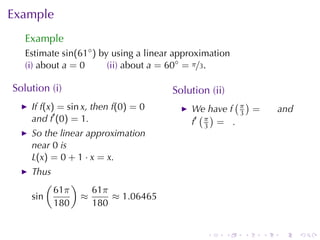
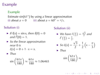
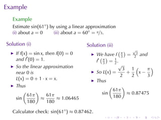
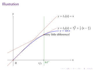
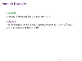
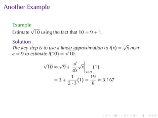
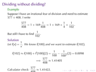
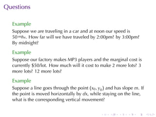
Section	2.8
         Linear	Approximation	and
                Differentials

                 V63.0121.027, Calculus	I


                    October	13, 2009


Announcements
   Midterm	Thursday	on	Sections	1.1–2.4

                                          .   .   .   .   .   .
Outline


  The	linear	approximation	of	a	function	near	a	point
     Examples


  Differentials
      The	not-so-big	idea
      Using	differentials	to	estimate	error


  Midterm	Review


  Advanced	Examples


                                              .   .     .   .   .   .
The	Big	Idea


   Question
   Let f be	differentiable	at a. What	linear	function	best
   approximates f near a?


                                                 .    .      .   .   .   .
The	Big	Idea


   Question
   Let f be	differentiable	at a. What	linear	function	best
   approximates f near a?

   Answer
   The	tangent	line, of	course!


                                                 .    .      .   .   .   .
The	Big	Idea


   Question
   Let f be	differentiable	at a. What	linear	function	best
   approximates f near a?

   Answer
   The	tangent	line, of	course!

   Question
   What	is	the	equation	for	the	line	tangent	to y = f(x) at (a, f(a))?

   Answer

                        L(x) = f(a) + f′ (a)(x − a)


                                                  .   .      .   .   .   .
Example
  Example
  Estimate sin(61◦ ) by	using	a	linear	approximation
  (i) about a = 0      (ii) about a = 60◦ = π/3.


                                              .   .    .   .   .   .
Example
   Example
   Estimate sin(61◦ ) by	using	a	linear	approximation
   (i) about a = 0      (ii) about a = 60◦ = π/3.

Solution	(i)
    If f(x) = sin x, then f(0) = 0
    and f′ (0) = 1.
    So	the	linear	approximation
    near 0 is
    L(x) = 0 + 1 · x = x.
    Thus
        (     )
          61π     61π
    sin         ≈     ≈ 1.06465
          180     180


                                               .   .    .   .   .   .
Example
   Example
   Estimate sin(61◦ ) by	using	a	linear	approximation
   (i) about a = 0      (ii) about a = 60◦ = π/3.

Solution	(i)                          Solution	(ii)
                                                    ( )
    If f(x) = sin x, then f(0) = 0         We	have f π =          and
    and f′ (0) = 1.                          ( )     3
                                           f′ π = .
                                              3
    So	the	linear	approximation
    near 0 is
    L(x) = 0 + 1 · x = x.
    Thus
        (     )
          61π     61π
    sin         ≈     ≈ 1.06465
          180     180


                                               .      .   .   .   .     .
Example
   Example
   Estimate sin(61◦ ) by	using	a	linear	approximation
   (i) about a = 0      (ii) about a = 60◦ = π/3.

Solution	(i)                          Solution	(ii)
                                                    ( )       √
    If f(x) = sin x, then f(0) = 0         We	have f π =       3
                                                                   and
    and f′ (0) = 1.                          ( )     3        2
                                           f′ π = .
                                              3
    So	the	linear	approximation
    near 0 is
    L(x) = 0 + 1 · x = x.
    Thus
        (     )
          61π     61π
    sin         ≈     ≈ 1.06465
          180     180


                                               .      .   .   .    .     .
Example
   Example
   Estimate sin(61◦ ) by	using	a	linear	approximation
   (i) about a = 0      (ii) about a = 60◦ = π/3.

Solution	(i)                          Solution	(ii)
                                                     ( )      √
    If f(x) = sin x, then f(0) = 0         We	have f π =       3
                                                                   and
    and f′ (0) = 1.                          ( )      3       2
                                           f′ π = 1 .
                                              3   2
    So	the	linear	approximation
    near 0 is                              So L(x) =
    L(x) = 0 + 1 · x = x.
    Thus
        (     )
          61π     61π
    sin         ≈     ≈ 1.06465
          180     180


                                               .      .   .   .    .     .
Example
   Example
   Estimate sin(61◦ ) by	using	a	linear	approximation
   (i) about a = 0      (ii) about a = 60◦ = π/3.

Solution	(i)                          Solution	(ii)
                                                      ( ) √
    If f(x) = sin x, then f(0) = 0         We	have f π = 23 and
    and f′ (0) = 1.                          ( )       3
                                           f′ π = 1 .
                                              3     2
                                                      √
    So	the	linear	approximation                         3 1(    π)
    near 0 is                              So L(x) =     +   x−
                                                       2   2    3
    L(x) = 0 + 1 · x = x.
    Thus
        (     )
          61π     61π
    sin         ≈     ≈ 1.06465
          180     180


                                               .      .   .   .   .   .
Example
   Example
   Estimate sin(61◦ ) by	using	a	linear	approximation
   (i) about a = 0      (ii) about a = 60◦ = π/3.

Solution	(i)                          Solution	(ii)
                                                       ( ) √
    If f(x) = sin x, then f(0) = 0         We	have f π = 23 and
    and f′ (0) = 1.                          ( )        3
                                           f′ π = 1 .
                                              3      2
                                                       √
    So	the	linear	approximation                          3 1(     π)
    near 0 is                              So L(x) =       +   x−
                                                        2    2    3
    L(x) = 0 + 1 · x = x.                  Thus
    Thus                                          (      )
        (     )                                     61π
          61π     61π                         sin          ≈
    sin         ≈     ≈ 1.06465                     180
          180     180


                                               .      .   .   .   .   .
Example
   Example
   Estimate sin(61◦ ) by	using	a	linear	approximation
   (i) about a = 0      (ii) about a = 60◦ = π/3.

Solution	(i)                          Solution	(ii)
                                                       ( ) √
    If f(x) = sin x, then f(0) = 0         We	have f π = 23 and
    and f′ (0) = 1.                          ( )        3
                                           f′ π = 1 .
                                              3      2
                                                       √
    So	the	linear	approximation                          3 1(      π)
    near 0 is                              So L(x) =       +    x−
                                                        2    2     3
    L(x) = 0 + 1 · x = x.                  Thus
    Thus                                          (      )
        (     )                                     61π
          61π     61π                         sin          ≈ 0.87475
    sin         ≈     ≈ 1.06465                     180
          180     180

   Calculator	check: sin(61◦ ) ≈
                                               .      .   .   .   .   .
Example
   Example
   Estimate sin(61◦ ) by	using	a	linear	approximation
   (i) about a = 0      (ii) about a = 60◦ = π/3.

Solution	(i)                          Solution	(ii)
                                                        ( ) √
    If f(x) = sin x, then f(0) = 0          We	have f π = 23 and
    and f′ (0) = 1.                           ( )        3
                                            f′ π = 1 .
                                               3      2
                                                        √
    So	the	linear	approximation                           3 1(      π)
    near 0 is                               So L(x) =       +    x−
                                                         2    2     3
    L(x) = 0 + 1 · x = x.                   Thus
    Thus                                           (      )
        (     )                                      61π
          61π     61π                          sin          ≈ 0.87475
    sin         ≈     ≈ 1.06465                      180
          180     180

   Calculator	check: sin(61◦ ) ≈ 0.87462.
                                               .      .   .   .   .   .
Illustration

       y
       .


                      y
                      . = sin x


       .                              x
                                      .
               . 1◦
               6

                      .    .      .       .   .   .
Illustration

       y
       .
                      y
                      . = L1 (x) = x


                       y
                       . = sin x


       .                               x
                                       .
           0
           .   . 1◦
               6

                        .   .      .       .   .   .
Illustration

       y
       .
                                         y
                                         . = L1 (x) = x


               b
               . ig	difference!           y
                                          . = sin x


       .                                                  x
                                                          .
           0
           .                      . 1◦
                                  6

                                           .   .      .       .   .   .
Illustration

       y
       .
                                y
                                . = L1 (x) = x


                                               √
                                                    3       1
                                                                (                )
                                y
                                . = L2 (x) =       2    +   2       x−       π
                                                                             3
                                  y
                                  . = sin x
                     .


       .             .                         x
                                               .
           0
           .   .
               π/3       . 1◦
                         6

                                  .   .    .            .       .        .
Illustration

       y
       .
                                  y
                                  . = L1 (x) = x


                                                   √
                                                        3       1
                                                                    (                )
                                    y
                                    . = L2 (x) =       2    +   2       x−       π
                                                                                 3
                                       y
                                       . = sin x
                     . . ery	little	difference!
                       v


       .             .                             x
                                                   .
           0
           .   .
               π/3       . 1◦
                         6

                                    .     .    .            .       .        .
Another	Example

  Example
             √
  Estimate       10 using	the	fact	that 10 = 9 + 1.


                                                  .   .   .   .   .   .
Another	Example

  Example
             √
  Estimate       10 using	the	fact	that 10 = 9 + 1.

  Solution                                                    √
  The	key	step	is	to	use	a	linear	approximation	to f(x) =
                              √                                   x near
  a = 9 to	estimate f(10) = 10.


                                                  .   .   .        .   .   .
Another	Example

  Example
             √
  Estimate       10 using	the	fact	that 10 = 9 + 1.

  Solution                                                    √
  The	key	step	is	to	use	a	linear	approximation	to f(x) =
                              √                                   x near
  a = 9 to	estimate f(10) = 10.
                     √          √d√
                         10 ≈       9+x     (1)
                                 dx     x=9
                                1         19
                           =3+     (1 ) =     ≈ 3.167
                               2·3         6


                                                  .   .   .        .   .   .
Another	Example

  Example
             √
  Estimate       10 using	the	fact	that 10 = 9 + 1.

  Solution                                                    √
  The	key	step	is	to	use	a	linear	approximation	to f(x) =
                              √                                   x near
  a = 9 to	estimate f(10) = 10.
                     √          √  d√
                         10 ≈       9+  x     (1)
                                   dx     x=9
                                  1         19
                             =3+     (1 ) =     ≈ 3.167
                                 2·3         6
           (        )2
               19
  Check:                 =
                6


                                                  .   .   .        .   .   .
Another	Example

  Example
             √
  Estimate       10 using	the	fact	that 10 = 9 + 1.

  Solution                                                     √
  The	key	step	is	to	use	a	linear	approximation	to f(x) =
                              √                                    x near
  a = 9 to	estimate f(10) = 10.
                     √           √  d√
                         10 ≈        9+  x     (1)
                                    dx     x=9
                                   1         19
                              =3+     (1 ) =     ≈ 3.167
                                  2·3         6
           (        )2
               19            361
  Check:                 =       .
                6             36


                                                  .   .    .        .   .   .
Dividing	without	dividing?
   Example
   Suppose	I have	an	irrational	fear	of	division	and	need	to	estimate
   577 ÷ 408. I write
               577            1             1  1
                   = 1 + 169     = 1 + 169 × ×    .
               408           408            4 102
                              1
   But	still	I have	to	find       .
                             102


                                               .    .    .   .    .     .
Dividing	without	dividing?
   Example
   Suppose	I have	an	irrational	fear	of	division	and	need	to	estimate
   577 ÷ 408. I write
                577            1             1  1
                    = 1 + 169     = 1 + 169 × ×    .
                408           408            4 102
                              1
   But	still	I have	to	find       .
                             102
   Solution
                1
   Let f(x) =     . We	know f(100) and	we	want	to	estimate f(102).
                x
                                            1   1
       f(102) ≈ f(100) + f′ (100)(2) =        −     (2) = 0.0098
                                           100 1002
                                     577
                             =⇒          ≈ 1.41405
                                     408
                       577
   Calculator	check:          ≈ 1.41422.             .   .   .   .   .   .
Outline


  The	linear	approximation	of	a	function	near	a	point
     Examples


  Differentials
      The	not-so-big	idea
      Using	differentials	to	estimate	error


  Midterm	Review


  Advanced	Examples


                                              .   .     .   .   .   .
Questions

  Example
  Suppose	we	are	traveling	in	a	car	and	at	noon	our	speed	is
  50 mi/hr. How	far	will	we	have	traveled	by	2:00pm? by	3:00pm?
  By	midnight?


                                            .   .    .   .   .    .
Answers


  Example
  Suppose	we	are	traveling	in	a	car	and	at	noon	our	speed	is
  50 mi/hr. How	far	will	we	have	traveled	by	2:00pm? by	3:00pm?
  By	midnight?


                                            .   .    .   .   .    .
Answers


  Example
  Suppose	we	are	traveling	in	a	car	and	at	noon	our	speed	is
  50 mi/hr. How	far	will	we	have	traveled	by	2:00pm? by	3:00pm?
  By	midnight?

  Answer
      100 mi
      150 mi
      600 mi	(?) (Is	it	reasonable	to	assume	12	hours	at	the	same
      speed?)


                                             .    .   .    .    .   .
Questions

  Example
  Suppose	we	are	traveling	in	a	car	and	at	noon	our	speed	is
  50 mi/hr. How	far	will	we	have	traveled	by	2:00pm? by	3:00pm?
  By	midnight?

  Example
  Suppose	our	factory	makes	MP3	players	and	the	marginal	cost	is
  currently	$50/lot. How	much	will	it	cost	to	make	2	more	lots? 3
  more	lots? 12	more	lots?


                                             .   .   .    .   .     .
Answers


  Example
  Suppose	our	factory	makes	MP3	players	and	the	marginal	cost	is
  currently	$50/lot. How	much	will	it	cost	to	make	2	more	lots? 3
  more	lots? 12	more	lots?

  Answer
      $100
      $150
      $600	(?)


                                             .   .   .    .   .     .
Questions

  Example
  Suppose	we	are	traveling	in	a	car	and	at	noon	our	speed	is
  50 mi/hr. How	far	will	we	have	traveled	by	2:00pm? by	3:00pm?
  By	midnight?

  Example
  Suppose	our	factory	makes	MP3	players	and	the	marginal	cost	is
  currently	$50/lot. How	much	will	it	cost	to	make	2	more	lots? 3
  more	lots? 12	more	lots?

  Example
  Suppose	a	line	goes	through	the	point (x0 , y0 ) and	has	slope m. If
  the	point	is	moved	horizontally	by dx, while	staying	on	the	line,
  what	is	the	corresponding	vertical	movement?


                                               .    .    .   .    .      .
Answers


  Example
  Suppose	a	line	goes	through	the	point (x0 , y0 ) and	has	slope m. If
  the	point	is	moved	horizontally	by dx, while	staying	on	the	line,
  what	is	the	corresponding	vertical	movement?


                                               .    .    .   .    .      .
Answers


  Example
  Suppose	a	line	goes	through	the	point (x0 , y0 ) and	has	slope m. If
  the	point	is	moved	horizontally	by dx, while	staying	on	the	line,
  what	is	the	corresponding	vertical	movement?

  Answer
  The	slope	of	the	line	is
                                    rise
                               m=
                                    run
  We	are	given	a	“run”	of dx, so	the	corresponding	“rise”	is m dx.


                                               .    .    .   .    .      .
Differentials	are	another	way	to	express	derivatives


   f(x + ∆x) − f(x) ≈ f′ (x) ∆x   y
                                  .
          ∆y                dy

  Rename ∆x = dx, so	we	can
  write	this	as
                                                      .
       ∆y ≈ dy = f′ (x)dx.                                        .
                                                                  dy
                                                          .
                                                          ∆y

  And	this	looks	a	lot	like	the           .
                                           .
                                           dx = ∆ x
  Leibniz-Newton	identity

            dy                    .                                        x
                                                                           .
               = f ′ (x )
            dx                        x x
                                      . . + ∆x


                                      .         .             .        .       .   .
Differentials	are	another	way	to	express	derivatives


   f(x + ∆x) − f(x) ≈ f′ (x) ∆x          y
                                         .
          ∆y                dy

  Rename ∆x = dx, so	we	can
  write	this	as
                                                               .
       ∆y ≈ dy = f′ (x)dx.                                                 .
                                                                           dy
                                                                   .
                                                                   ∆y

  And	this	looks	a	lot	like	the                    .
                                                    .
                                                    dx = ∆ x
  Leibniz-Newton	identity

            dy                            .                                         x
                                                                                    .
               = f ′ (x )
            dx                                 x x
                                               . . + ∆x
   Linear	approximation	means ∆y ≈ dy = f′ (x0 ) dx near x0 .

                                               .         .             .        .       .   .
Using	differentials	to	estimate	error


                                 y
                                 .
  If y = f(x), x0 and ∆x is
  known, and	an	estimate	of
  ∆y is	desired:
      Approximate: ∆y ≈ dy
                                                        .
      Differentiate:                                                .
                                                                    dy
      dy = f′ (x) dx                                        .
                                                            ∆y

                                            .
      Evaluate	at x = x0 and                 .
                                             dx = ∆ x

      dx = ∆x.

                                  .                                          x
                                                                             .
                                        x x
                                        . . + ∆x


                                        .         .             .        .       .   .
Example
A sheet	of	plywood	measures 8 ft × 4 ft. Suppose	our
plywood-cutting	machine	will	cut	a	rectangle	whose	width	is
exactly	half	its	length, but	the	length	is	prone	to	errors. If	the
length	is	off	by 1 in, how	bad	can	the	area	of	the	sheet	be	off	by?


                                             .    .    .   .    .     .
Example
A sheet	of	plywood	measures 8 ft × 4 ft. Suppose	our
plywood-cutting	machine	will	cut	a	rectangle	whose	width	is
exactly	half	its	length, but	the	length	is	prone	to	errors. If	the
length	is	off	by 1 in, how	bad	can	the	area	of	the	sheet	be	off	by?

Solution
            1
Write A(ℓ) = ℓ2 . We	want	to	know ∆A when ℓ = 8 ft and
            2
∆ℓ = 1 in.


                                             .    .    .   .    .     .
Example
A sheet	of	plywood	measures 8 ft × 4 ft. Suppose	our
plywood-cutting	machine	will	cut	a	rectangle	whose	width	is
exactly	half	its	length, but	the	length	is	prone	to	errors. If	the
length	is	off	by 1 in, how	bad	can	the	area	of	the	sheet	be	off	by?

Solution
             1
Write A(ℓ) = ℓ2 . We	want	to	know ∆A when ℓ = 8 ft and
             2
∆ℓ = 1 in.          ( )
                      97     9409
  (I) A(ℓ + ∆ℓ) = A       =       So
                      12     288
            9409
      ∆A =        − 32 ≈ 0.6701.
             288


                                             .    .    .   .    .     .
Example
A sheet	of	plywood	measures 8 ft × 4 ft. Suppose	our
plywood-cutting	machine	will	cut	a	rectangle	whose	width	is
exactly	half	its	length, but	the	length	is	prone	to	errors. If	the
length	is	off	by 1 in, how	bad	can	the	area	of	the	sheet	be	off	by?

Solution
              1
Write A(ℓ) = ℓ2 . We	want	to	know ∆A when ℓ = 8 ft and
              2
∆ℓ = 1 in.            ( )
                        97     9409
  (I) A(ℓ + ∆ℓ) = A          =       So
                        12     288
            9409
      ∆A =          − 32 ≈ 0.6701.
             288
      dA
 (II)     = ℓ, so dA = ℓ dℓ, which	should	be	a	good	estimate	for
      dℓ
                                  1
      ∆ℓ. When ℓ = 8 and dℓ = 12 , we	have
            8     2
      dA = 12 = 3 ≈ 0.667. So	we	get	estimates	close	to	the
      hundredth	of	a	square	foot.
                                             .    .    .   .    .     .
Why?


  Why	use	linear	approximations dy when	the	actual	difference ∆y
  is	known?
       Linear	approximation	is	quick	and	reliable. Finding ∆y
       exactly	depends	on	the	function.
       These	examples	are	overly	simple. See	the	“Advanced
       Examples”	later.
       In	real	life, sometimes	only f(a) and f′ (a) are	known, and	not
       the	general f(x).


                                               .    .    .   .    .      .
Outline


  The	linear	approximation	of	a	function	near	a	point
     Examples


  Differentials
      The	not-so-big	idea
      Using	differentials	to	estimate	error


  Midterm	Review


  Advanced	Examples


                                              .   .     .   .   .   .
Midterm	Facts

     Covers	sections	1.1–2.4
     (Limits, Derivatives,
     Differentiation	up	to
     Quotient	Rule)
     Calculator	free
     Has	about	7	problems
     each	could	have
     multiple	parts
     Some	fixed-response,
     some	free-response
     To	study:
         outline
         do	problems
         metacognition
         ask	questions!

                               .   .   .   .   .   .
Outline


  The	linear	approximation	of	a	function	near	a	point
     Examples


  Differentials
      The	not-so-big	idea
      Using	differentials	to	estimate	error


  Midterm	Review


  Advanced	Examples


                                              .   .     .   .   .   .
Gravitation
Pencils	down!
    Example
         Drop	a	1 kg	ball	off	the	roof	of	the	Silver	Center	(50m	high).
         We	usually	say	that	a	falling	object	feels	a	force F = −mg
         from	gravity.


                                                  .   .    .    .   .     .
Gravitation
Pencils	down!
    Example
         Drop	a	1 kg	ball	off	the	roof	of	the	Silver	Center	(50m	high).
         We	usually	say	that	a	falling	object	feels	a	force F = −mg
         from	gravity.
         In	fact, the	force	felt	is
                                                   GMm
                                      F (r ) = −       ,
                                                    r2
         where M is	the	mass	of	the	earth	and r is	the	distance	from
         the	center	of	the	earth	to	the	object. G is	a	constant.
                                                GMm
         At r = re the	force	really	is F(re ) =      = −mg.
                                                 r2
                                                  e
         What	is	the	maximum	error	in	replacing	the	actual	force	felt
         at	the	top	of	the	building F(re + ∆r) by	the	force	felt	at
         ground	level F(re )? The	relative	error? The	percentage	error?
                                                           .   .   .   .   .   .
Solution
We	wonder	if ∆F = F(re + ∆r) − F(re ) is	small.
    Using	a	linear	approximation,

                              dF            GMm
                  ∆F ≈ dF =          dr = 2 3 dr
                              dr r           re
                              ( e )
                               GMm dr             ∆r
                            =      2
                                            = 2mg
                                 re      re       re

                        ∆F      ∆r
    The	relative	error	is  ≈ −2
                        F        re
    re = 6378.1 km. If ∆r = 50 m,
    ∆F      ∆r         50
       ≈ −2    = −2         = −1.56 × 10−5 = −0.00156%
     F      re      6378100


                                            .     .    .   .   .   .
Systematic	linear	approximation

      √                          √
          2 is	irrational, but       9/4   is	rational	and 9/4 is	close	to 2.


                                                         .    .    .    .       .   .
Systematic	linear	approximation

      √                          √
          2 is	irrational, but       9/4   is	rational	and 9/4 is	close	to 2. So
               √        √                   √               1             17
                   2=    9/4   − 1/4 ≈          9/4   +          (−1/4) =
                                                          2(3/2)          12


                                                              .   .    .   .   .   .
Systematic	linear	approximation

      √                          √
          2 is	irrational, but       9/4   is	rational	and 9/4 is	close	to 2. So
               √        √                   √               1             17
                   2=    9/4   − 1/4 ≈          9/4   +          (−1/4) =
                                                          2(3/2)          12


      This	is	a	better	approximation	since (17/12)2 = 289/144


                                                              .   .    .   .   .   .
Systematic	linear	approximation

      √                             √
          2 is	irrational, but          9/4   is	rational	and 9/4 is	close	to 2. So
               √         √                     √               1             17
                   2=        9/4   − 1/4 ≈         9/4   +          (−1/4) =
                                                             2(3/2)          12


      This	is	a	better	approximation	since (17/12)2 = 289/144
      Do	it	again!
      √        √                              √                  1
          2=       289/144   − 1/144 ≈            289/144+             (−1/144) = 577/408
                                                              2(17/12)
              (         )2
                  577            332, 929             1
      Now                    =            which	is          away	from 2.
                  408            166, 464          166, 464


                                                                 .   .    .    .    .   .
Illustration	of	the	previous	example


                 .


                                       .   .   .   .   .   .
Illustration	of	the	previous	example


                 .


                                       .   .   .   .   .   .
Illustration	of	the	previous	example


                 .
                             2
                             .


                                       .   .   .   .   .   .
Illustration	of	the	previous	example


                                 .


                 .
                             2
                             .


                                       .   .   .   .   .   .
Illustration	of	the	previous	example


                                 .


                 .
                             2
                             .


                                       .   .   .   .   .   .
Illustration	of	the	previous	example


                        . 2, 17 )
                        ( 12
                                    . .


                 .
                                    2
                                    .


                                          .   .   .   .   .   .
Illustration	of	the	previous	example


                                       .
                     . 2, 17/12)
                     (
                                   .       (9 2
                                           . 4, 3)


                                            .        .   .   .   .   .
Illustration	of	the	previous	example


                                                 .
                     . 2, 17/12)
                     (
                                   ..              . 9, 3)
                                                   (
                                        ( 289 17 ) 4 2
                                        . 144 , 12


                                                     .       .   .   .   .   .
Illustration	of	the	previous	example


                                               .
                     . 2, 17/12)
                     (
                                 ..              . 9, 3)
                                                 (
                      ( 577 ) ( 289 17 ) 4 2
                      . 2, 408      . 144 , 12


                                                  .        .   .   .   .   .

Lesson 12: Linear Approximation and Differentials

  • 1.
    Section 2.8 Linear Approximation and Differentials V63.0121.027, Calculus I October 13, 2009 Announcements Midterm Thursday on Sections 1.1–2.4 . . . . . .
  • 2.
    Outline The linear approximation of a function near a point Examples Differentials The not-so-big idea Using differentials to estimate error Midterm Review Advanced Examples . . . . . .
  • 3.
    The Big Idea Question Let f be differentiable at a. What linear function best approximates f near a? . . . . . .
  • 4.
    The Big Idea Question Let f be differentiable at a. What linear function best approximates f near a? Answer The tangent line, of course! . . . . . .
  • 5.
    The Big Idea Question Let f be differentiable at a. What linear function best approximates f near a? Answer The tangent line, of course! Question What is the equation for the line tangent to y = f(x) at (a, f(a))? . . . . . .
  • 6.
    The Big Idea Question Let f be differentiable at a. What linear function best approximates f near a? Answer The tangent line, of course! Question What is the equation for the line tangent to y = f(x) at (a, f(a))? Answer L(x) = f(a) + f′ (a)(x − a) . . . . . .
  • 7.
    Example Example Estimate sin(61◦ ) by using a linear approximation (i) about a = 0 (ii) about a = 60◦ = π/3. . . . . . .
  • 8.
    Example Example Estimate sin(61◦ ) by using a linear approximation (i) about a = 0 (ii) about a = 60◦ = π/3. Solution (i) If f(x) = sin x, then f(0) = 0 and f′ (0) = 1. So the linear approximation near 0 is L(x) = 0 + 1 · x = x. Thus ( ) 61π 61π sin ≈ ≈ 1.06465 180 180 . . . . . .
  • 9.
    Example Example Estimate sin(61◦ ) by using a linear approximation (i) about a = 0 (ii) about a = 60◦ = π/3. Solution (i) Solution (ii) ( ) If f(x) = sin x, then f(0) = 0 We have f π = and and f′ (0) = 1. ( ) 3 f′ π = . 3 So the linear approximation near 0 is L(x) = 0 + 1 · x = x. Thus ( ) 61π 61π sin ≈ ≈ 1.06465 180 180 . . . . . .
  • 10.
    Example Example Estimate sin(61◦ ) by using a linear approximation (i) about a = 0 (ii) about a = 60◦ = π/3. Solution (i) Solution (ii) ( ) √ If f(x) = sin x, then f(0) = 0 We have f π = 3 and and f′ (0) = 1. ( ) 3 2 f′ π = . 3 So the linear approximation near 0 is L(x) = 0 + 1 · x = x. Thus ( ) 61π 61π sin ≈ ≈ 1.06465 180 180 . . . . . .
  • 11.
    Example Example Estimate sin(61◦ ) by using a linear approximation (i) about a = 0 (ii) about a = 60◦ = π/3. Solution (i) Solution (ii) ( ) √ If f(x) = sin x, then f(0) = 0 We have f π = 3 and and f′ (0) = 1. ( ) 3 2 f′ π = 1 . 3 2 So the linear approximation near 0 is L(x) = 0 + 1 · x = x. Thus ( ) 61π 61π sin ≈ ≈ 1.06465 180 180 . . . . . .
  • 12.
    Example Example Estimate sin(61◦ ) by using a linear approximation (i) about a = 0 (ii) about a = 60◦ = π/3. Solution (i) Solution (ii) ( ) √ If f(x) = sin x, then f(0) = 0 We have f π = 3 and and f′ (0) = 1. ( ) 3 2 f′ π = 1 . 3 2 So the linear approximation near 0 is So L(x) = L(x) = 0 + 1 · x = x. Thus ( ) 61π 61π sin ≈ ≈ 1.06465 180 180 . . . . . .
  • 13.
    Example Example Estimate sin(61◦ ) by using a linear approximation (i) about a = 0 (ii) about a = 60◦ = π/3. Solution (i) Solution (ii) ( ) √ If f(x) = sin x, then f(0) = 0 We have f π = 23 and and f′ (0) = 1. ( ) 3 f′ π = 1 . 3 2 √ So the linear approximation 3 1( π) near 0 is So L(x) = + x− 2 2 3 L(x) = 0 + 1 · x = x. Thus ( ) 61π 61π sin ≈ ≈ 1.06465 180 180 . . . . . .
  • 14.
    Example Example Estimate sin(61◦ ) by using a linear approximation (i) about a = 0 (ii) about a = 60◦ = π/3. Solution (i) Solution (ii) ( ) √ If f(x) = sin x, then f(0) = 0 We have f π = 23 and and f′ (0) = 1. ( ) 3 f′ π = 1 . 3 2 √ So the linear approximation 3 1( π) near 0 is So L(x) = + x− 2 2 3 L(x) = 0 + 1 · x = x. Thus Thus ( ) ( ) 61π 61π 61π sin ≈ sin ≈ ≈ 1.06465 180 180 180 . . . . . .
  • 15.
    Example Example Estimate sin(61◦ ) by using a linear approximation (i) about a = 0 (ii) about a = 60◦ = π/3. Solution (i) Solution (ii) ( ) √ If f(x) = sin x, then f(0) = 0 We have f π = 23 and and f′ (0) = 1. ( ) 3 f′ π = 1 . 3 2 √ So the linear approximation 3 1( π) near 0 is So L(x) = + x− 2 2 3 L(x) = 0 + 1 · x = x. Thus Thus ( ) ( ) 61π 61π 61π sin ≈ 0.87475 sin ≈ ≈ 1.06465 180 180 180 . . . . . .
  • 16.
    Example Example Estimate sin(61◦ ) by using a linear approximation (i) about a = 0 (ii) about a = 60◦ = π/3. Solution (i) Solution (ii) ( ) √ If f(x) = sin x, then f(0) = 0 We have f π = 23 and and f′ (0) = 1. ( ) 3 f′ π = 1 . 3 2 √ So the linear approximation 3 1( π) near 0 is So L(x) = + x− 2 2 3 L(x) = 0 + 1 · x = x. Thus Thus ( ) ( ) 61π 61π 61π sin ≈ 0.87475 sin ≈ ≈ 1.06465 180 180 180 Calculator check: sin(61◦ ) ≈ . . . . . .
  • 17.
    Example Example Estimate sin(61◦ ) by using a linear approximation (i) about a = 0 (ii) about a = 60◦ = π/3. Solution (i) Solution (ii) ( ) √ If f(x) = sin x, then f(0) = 0 We have f π = 23 and and f′ (0) = 1. ( ) 3 f′ π = 1 . 3 2 √ So the linear approximation 3 1( π) near 0 is So L(x) = + x− 2 2 3 L(x) = 0 + 1 · x = x. Thus Thus ( ) ( ) 61π 61π 61π sin ≈ 0.87475 sin ≈ ≈ 1.06465 180 180 180 Calculator check: sin(61◦ ) ≈ 0.87462. . . . . . .
  • 18.
    Illustration y . y . = sin x . x . . 1◦ 6 . . . . . .
  • 19.
    Illustration y . y . = L1 (x) = x y . = sin x . x . 0 . . 1◦ 6 . . . . . .
  • 20.
    Illustration y . y . = L1 (x) = x b . ig difference! y . = sin x . x . 0 . . 1◦ 6 . . . . . .
  • 21.
    Illustration y . y . = L1 (x) = x √ 3 1 ( ) y . = L2 (x) = 2 + 2 x− π 3 y . = sin x . . . x . 0 . . π/3 . 1◦ 6 . . . . . .
  • 22.
    Illustration y . y . = L1 (x) = x √ 3 1 ( ) y . = L2 (x) = 2 + 2 x− π 3 y . = sin x . . ery little difference! v . . x . 0 . . π/3 . 1◦ 6 . . . . . .
  • 23.
    Another Example Example √ Estimate 10 using the fact that 10 = 9 + 1. . . . . . .
  • 24.
    Another Example Example √ Estimate 10 using the fact that 10 = 9 + 1. Solution √ The key step is to use a linear approximation to f(x) = √ x near a = 9 to estimate f(10) = 10. . . . . . .
  • 25.
    Another Example Example √ Estimate 10 using the fact that 10 = 9 + 1. Solution √ The key step is to use a linear approximation to f(x) = √ x near a = 9 to estimate f(10) = 10. √ √d√ 10 ≈ 9+x (1) dx x=9 1 19 =3+ (1 ) = ≈ 3.167 2·3 6 . . . . . .
  • 26.
    Another Example Example √ Estimate 10 using the fact that 10 = 9 + 1. Solution √ The key step is to use a linear approximation to f(x) = √ x near a = 9 to estimate f(10) = 10. √ √ d√ 10 ≈ 9+ x (1) dx x=9 1 19 =3+ (1 ) = ≈ 3.167 2·3 6 ( )2 19 Check: = 6 . . . . . .
  • 27.
    Another Example Example √ Estimate 10 using the fact that 10 = 9 + 1. Solution √ The key step is to use a linear approximation to f(x) = √ x near a = 9 to estimate f(10) = 10. √ √ d√ 10 ≈ 9+ x (1) dx x=9 1 19 =3+ (1 ) = ≈ 3.167 2·3 6 ( )2 19 361 Check: = . 6 36 . . . . . .
  • 28.
    Dividing without dividing? Example Suppose I have an irrational fear of division and need to estimate 577 ÷ 408. I write 577 1 1 1 = 1 + 169 = 1 + 169 × × . 408 408 4 102 1 But still I have to find . 102 . . . . . .
  • 29.
    Dividing without dividing? Example Suppose I have an irrational fear of division and need to estimate 577 ÷ 408. I write 577 1 1 1 = 1 + 169 = 1 + 169 × × . 408 408 4 102 1 But still I have to find . 102 Solution 1 Let f(x) = . We know f(100) and we want to estimate f(102). x 1 1 f(102) ≈ f(100) + f′ (100)(2) = − (2) = 0.0098 100 1002 577 =⇒ ≈ 1.41405 408 577 Calculator check: ≈ 1.41422. . . . . . .
  • 30.
    Outline The linear approximation of a function near a point Examples Differentials The not-so-big idea Using differentials to estimate error Midterm Review Advanced Examples . . . . . .
  • 31.
    Questions Example Suppose we are traveling in a car and at noon our speed is 50 mi/hr. How far will we have traveled by 2:00pm? by 3:00pm? By midnight? . . . . . .
  • 32.
    Answers Example Suppose we are traveling in a car and at noon our speed is 50 mi/hr. How far will we have traveled by 2:00pm? by 3:00pm? By midnight? . . . . . .
  • 33.
    Answers Example Suppose we are traveling in a car and at noon our speed is 50 mi/hr. How far will we have traveled by 2:00pm? by 3:00pm? By midnight? Answer 100 mi 150 mi 600 mi (?) (Is it reasonable to assume 12 hours at the same speed?) . . . . . .
  • 34.
    Questions Example Suppose we are traveling in a car and at noon our speed is 50 mi/hr. How far will we have traveled by 2:00pm? by 3:00pm? By midnight? Example Suppose our factory makes MP3 players and the marginal cost is currently $50/lot. How much will it cost to make 2 more lots? 3 more lots? 12 more lots? . . . . . .
  • 35.
    Answers Example Suppose our factory makes MP3 players and the marginal cost is currently $50/lot. How much will it cost to make 2 more lots? 3 more lots? 12 more lots? Answer $100 $150 $600 (?) . . . . . .
  • 36.
    Questions Example Suppose we are traveling in a car and at noon our speed is 50 mi/hr. How far will we have traveled by 2:00pm? by 3:00pm? By midnight? Example Suppose our factory makes MP3 players and the marginal cost is currently $50/lot. How much will it cost to make 2 more lots? 3 more lots? 12 more lots? Example Suppose a line goes through the point (x0 , y0 ) and has slope m. If the point is moved horizontally by dx, while staying on the line, what is the corresponding vertical movement? . . . . . .
  • 37.
    Answers Example Suppose a line goes through the point (x0 , y0 ) and has slope m. If the point is moved horizontally by dx, while staying on the line, what is the corresponding vertical movement? . . . . . .
  • 38.
    Answers Example Suppose a line goes through the point (x0 , y0 ) and has slope m. If the point is moved horizontally by dx, while staying on the line, what is the corresponding vertical movement? Answer The slope of the line is rise m= run We are given a “run” of dx, so the corresponding “rise” is m dx. . . . . . .
  • 39.
    Differentials are another way to express derivatives f(x + ∆x) − f(x) ≈ f′ (x) ∆x y . ∆y dy Rename ∆x = dx, so we can write this as . ∆y ≈ dy = f′ (x)dx. . dy . ∆y And this looks a lot like the . . dx = ∆ x Leibniz-Newton identity dy . x . = f ′ (x ) dx x x . . + ∆x . . . . . .
  • 40.
    Differentials are another way to express derivatives f(x + ∆x) − f(x) ≈ f′ (x) ∆x y . ∆y dy Rename ∆x = dx, so we can write this as . ∆y ≈ dy = f′ (x)dx. . dy . ∆y And this looks a lot like the . . dx = ∆ x Leibniz-Newton identity dy . x . = f ′ (x ) dx x x . . + ∆x Linear approximation means ∆y ≈ dy = f′ (x0 ) dx near x0 . . . . . . .
  • 41.
    Using differentials to estimate error y . If y = f(x), x0 and ∆x is known, and an estimate of ∆y is desired: Approximate: ∆y ≈ dy . Differentiate: . dy dy = f′ (x) dx . ∆y . Evaluate at x = x0 and . dx = ∆ x dx = ∆x. . x . x x . . + ∆x . . . . . .
  • 42.
    Example A sheet of plywood measures 8ft × 4 ft. Suppose our plywood-cutting machine will cut a rectangle whose width is exactly half its length, but the length is prone to errors. If the length is off by 1 in, how bad can the area of the sheet be off by? . . . . . .
  • 43.
    Example A sheet of plywood measures 8ft × 4 ft. Suppose our plywood-cutting machine will cut a rectangle whose width is exactly half its length, but the length is prone to errors. If the length is off by 1 in, how bad can the area of the sheet be off by? Solution 1 Write A(ℓ) = ℓ2 . We want to know ∆A when ℓ = 8 ft and 2 ∆ℓ = 1 in. . . . . . .
  • 44.
    Example A sheet of plywood measures 8ft × 4 ft. Suppose our plywood-cutting machine will cut a rectangle whose width is exactly half its length, but the length is prone to errors. If the length is off by 1 in, how bad can the area of the sheet be off by? Solution 1 Write A(ℓ) = ℓ2 . We want to know ∆A when ℓ = 8 ft and 2 ∆ℓ = 1 in. ( ) 97 9409 (I) A(ℓ + ∆ℓ) = A = So 12 288 9409 ∆A = − 32 ≈ 0.6701. 288 . . . . . .
  • 45.
    Example A sheet of plywood measures 8ft × 4 ft. Suppose our plywood-cutting machine will cut a rectangle whose width is exactly half its length, but the length is prone to errors. If the length is off by 1 in, how bad can the area of the sheet be off by? Solution 1 Write A(ℓ) = ℓ2 . We want to know ∆A when ℓ = 8 ft and 2 ∆ℓ = 1 in. ( ) 97 9409 (I) A(ℓ + ∆ℓ) = A = So 12 288 9409 ∆A = − 32 ≈ 0.6701. 288 dA (II) = ℓ, so dA = ℓ dℓ, which should be a good estimate for dℓ 1 ∆ℓ. When ℓ = 8 and dℓ = 12 , we have 8 2 dA = 12 = 3 ≈ 0.667. So we get estimates close to the hundredth of a square foot. . . . . . .
  • 46.
    Why? Why use linear approximationsdy when the actual difference ∆y is known? Linear approximation is quick and reliable. Finding ∆y exactly depends on the function. These examples are overly simple. See the “Advanced Examples” later. In real life, sometimes only f(a) and f′ (a) are known, and not the general f(x). . . . . . .
  • 47.
    Outline The linear approximation of a function near a point Examples Differentials The not-so-big idea Using differentials to estimate error Midterm Review Advanced Examples . . . . . .
  • 48.
    Midterm Facts Covers sections 1.1–2.4 (Limits, Derivatives, Differentiation up to Quotient Rule) Calculator free Has about 7 problems each could have multiple parts Some fixed-response, some free-response To study: outline do problems metacognition ask questions! . . . . . .
  • 49.
    Outline The linear approximation of a function near a point Examples Differentials The not-so-big idea Using differentials to estimate error Midterm Review Advanced Examples . . . . . .
  • 50.
    Gravitation Pencils down! Example Drop a 1 kg ball off the roof of the Silver Center (50m high). We usually say that a falling object feels a force F = −mg from gravity. . . . . . .
  • 51.
    Gravitation Pencils down! Example Drop a 1 kg ball off the roof of the Silver Center (50m high). We usually say that a falling object feels a force F = −mg from gravity. In fact, the force felt is GMm F (r ) = − , r2 where M is the mass of the earth and r is the distance from the center of the earth to the object. G is a constant. GMm At r = re the force really is F(re ) = = −mg. r2 e What is the maximum error in replacing the actual force felt at the top of the building F(re + ∆r) by the force felt at ground level F(re )? The relative error? The percentage error? . . . . . .
  • 52.
    Solution We wonder if ∆F =F(re + ∆r) − F(re ) is small. Using a linear approximation, dF GMm ∆F ≈ dF = dr = 2 3 dr dr r re ( e ) GMm dr ∆r = 2 = 2mg re re re ∆F ∆r The relative error is ≈ −2 F re re = 6378.1 km. If ∆r = 50 m, ∆F ∆r 50 ≈ −2 = −2 = −1.56 × 10−5 = −0.00156% F re 6378100 . . . . . .
  • 53.
    Systematic linear approximation √ √ 2 is irrational, but 9/4 is rational and 9/4 is close to 2. . . . . . .
  • 54.
    Systematic linear approximation √ √ 2 is irrational, but 9/4 is rational and 9/4 is close to 2. So √ √ √ 1 17 2= 9/4 − 1/4 ≈ 9/4 + (−1/4) = 2(3/2) 12 . . . . . .
  • 55.
    Systematic linear approximation √ √ 2 is irrational, but 9/4 is rational and 9/4 is close to 2. So √ √ √ 1 17 2= 9/4 − 1/4 ≈ 9/4 + (−1/4) = 2(3/2) 12 This is a better approximation since (17/12)2 = 289/144 . . . . . .
  • 56.
    Systematic linear approximation √ √ 2 is irrational, but 9/4 is rational and 9/4 is close to 2. So √ √ √ 1 17 2= 9/4 − 1/4 ≈ 9/4 + (−1/4) = 2(3/2) 12 This is a better approximation since (17/12)2 = 289/144 Do it again! √ √ √ 1 2= 289/144 − 1/144 ≈ 289/144+ (−1/144) = 577/408 2(17/12) ( )2 577 332, 929 1 Now = which is away from 2. 408 166, 464 166, 464 . . . . . .
  • 57.
  • 58.
  • 59.
  • 60.
  • 61.
  • 62.
    Illustration of the previous example . 2, 17 ) ( 12 . . . 2 . . . . . . .
  • 63.
    Illustration of the previous example . 2, 17 ) ( 12 . . . 2 . . . . . . .
  • 64.
    Illustration of the previous example . . 2, 17/12) ( . (9 2 . 4, 3) . . . . . .
  • 65.
    Illustration of the previous example . . 2, 17/12) ( .. . 9, 3) ( ( 289 17 ) 4 2 . 144 , 12 . . . . . .
  • 66.
    Illustration of the previous example . . 2, 17/12) ( .. . 9, 3) ( ( 577 ) ( 289 17 ) 4 2 . 2, 408 . 144 , 12 . . . . . .