SlideShare a Scribd company logo
1 of 104
Download to read offline
22 MAGNETISM
Figure 22.1 The magnificent spectacle of the Aurora Borealis, or northern lights, glows in the northern sky above Bear Lake near Eielson Air Force
Base, Alaska. Shaped by the Earth’s magnetic field, this light is produced by radiation spewed from solar storms. (credit: Senior Airman Joshua Strang,
via Flickr)
Chapter Outline
22.1. Magnets
22.2. Ferromagnets and Electromagnets
22.3. Magnetic Fields and Magnetic Field Lines
22.4. Magnetic Field Strength: Force on a Moving Charge in a Magnetic Field
22.5. Force on a Moving Charge in a Magnetic Field: Examples and Applications
22.6. The Hall Effect
22.7. Magnetic Force on a Current-Carrying Conductor
22.8. Torque on a Current Loop: Motors and Meters
22.9. Magnetic Fields Produced by Currents: Ampere’s Law
22.10. Magnetic Force between Two Parallel Conductors
22.11. More Applications of Magnetism
Connection for AP® Courses
Magnetism plays a major role in your everyday life. All electric motors, with uses as diverse as powering refrigerators, starting
cars, and moving elevators, contain magnets. Magnetic resonance imaging (MRI) has become an important diagnostic tool in the
field of medicine, and the use of magnetism to explore brain activity is a subject of contemporary research and development.
Other applications of magnetism include computer memory, levitation of high-speed trains, the aurora borealis, and, of course,
the first important historical use of magnetism: navigation. You will find all of these applications of magnetism linked by a small
number of underlying principles.
In this chapter, you will learn that both the internal properties of an object and the movement of charged particles can generate a
magnetic field, and you will learn why all magnetic fields have a north and south pole. You will also learn how magnetic fields
exert forces on objects, resulting in the magnetic alignment that makes a compass work. You will learn how we use this principle
to weigh the smallest of subatomic particles with precision and contain superheated plasma to facilitate nuclear fusion.
Big Idea 1 Objects and systems have properties such as mass and charge. Systems may have internal structure.
Enduring Understanding 1.E Materials have many macroscopic properties that result from the arrangement and interactions of
the atoms and molecules that make up the material.
Essential Knowledge 1.E.5 Matter has a property called magnetic permeability.
Chapter 22 | Magnetism 965
Essential Knowledge 1.E.6 Matter has a property called magnetic dipole moment.
Big Idea 2 Fields existing in space can be used to explain interactions.
Enduring Understanding 2.D A magnetic field is caused by a magnet or a moving electrically charged object. Magnetic fields
observed in nature always seem to be produced either by moving charged objects or by magnetic dipoles or combinations of
dipoles and never by single poles.
Essential Knowledge 2.D.1 The magnetic field exerts a force on a moving electrically charged object. That magnetic force is
perpendicular to the direction of the velocity of the object and to the magnetic field and is proportional to the magnitude of the
charge, the magnitude of the velocity, and the magnitude of the magnetic field. It also depends on the angle between the velocity
and the magnetic field vectors. Treatment is quantitative for angles of 0°, 90°, or 180° and qualitative for other angles.
Essential Knowledge 2.D.2 The magnetic field vectors around a straight wire that carries electric current are tangent to
concentric circles centered on that wire. The field has no component toward the current-carrying wire.
Essential Knowledge 2.D.3 A magnetic dipole placed in a magnetic field, such as the ones created by a magnet or the Earth, will
tend to align with the magnetic field vector.
Essential Knowledge 2.D.4 Ferromagnetic materials contain magnetic domains that are themselves magnets.
Big Idea 3 The interactions of an object with other objects can be described by forces.
Enduring Understanding 3.C At the macroscopic level, forces can be categorized as either long-range (action-at-a-distance)
forces or contact forces.
Essential Knowledge 3.C.3 A magnetic force results from the interaction of a moving charged object or a magnet with other
moving charged objects or another magnet.
Big Idea 4 Interactions between systems can result in changes in those systems.
Enduring Understanding 4.E The electric and magnetic properties of a system can change in response to the presence of, or
changes in, other objects or systems.
Essential Knowledge 4.E.1 The magnetic properties of some materials can be affected by magnetic fields at the system.
Students should focus on the underlying concepts and not the use of the vocabulary.
Figure 22.2 Engineering of technology like iPods would not be possible without a deep understanding of magnetism. (credit: Jesse! S?, Flickr)
22.1 Magnets
Learning Objectives
By the end of this section, you will be able to:
• Describe the difference between the north and south poles of a magnet.
• Describe how magnetic poles interact with each other.
966 Chapter 22 | Magnetism
This content is available for free at http://cnx.org/content/col11844/1.13
Figure 22.3 Magnets come in various shapes, sizes, and strengths. All have both a north pole and a south pole. There is never an isolated pole (a
monopole).
All magnets attract iron, such as that in a refrigerator door. However, magnets may attract or repel other magnets.
Experimentation shows that all magnets have two poles. If freely suspended, one pole will point toward the north. The two poles
are thus named the north magnetic pole and the south magnetic pole (or more properly, north-seeking and south-seeking
poles, for the attractions in those directions).
Universal Characteristics of Magnets and Magnetic Poles
It is a universal characteristic of all magnets that like poles repel and unlike poles attract. (Note the similarity with
electrostatics: unlike charges attract and like charges repel.)
Further experimentation shows that it is impossible to separate north and south poles in the manner that + and − charges
can be separated.
Figure 22.4 One end of a bar magnet is suspended from a thread that points toward north. The magnet’s two poles are labeled N and S for north-
seeking and south-seeking poles, respectively.
Misconception Alert: Earth’s Geographic North Pole Hides an S
The Earth acts like a very large bar magnet with its south-seeking pole near the geographic North Pole. That is why the
north pole of your compass is attracted toward the geographic north pole of the Earth—because the magnetic pole that is
near the geographic North Pole is actually a south magnetic pole! Confusion arises because the geographic term “North
Pole” has come to be used (incorrectly) for the magnetic pole that is near the North Pole. Thus, “North magnetic pole” is
actually a misnomer—it should be called the South magnetic pole.
Chapter 22 | Magnetism 967
Figure 22.5 Unlike poles attract, whereas like poles repel.
Figure 22.6 North and south poles always occur in pairs. Attempts to separate them result in more pairs of poles. If we continue to split the magnet, we
will eventually get down to an iron atom with a north pole and a south pole—these, too, cannot be separated.
Real World Connections: Dipoles and Monopoles
Figure 22.6 shows that no matter how many times you divide a magnet the resulting objects are always magnetic dipoles.
Formally, a magnetic dipole is an object (usually very small) with a north and south magnetic pole. Magnetic dipoles have a
vector property called magnetic momentum. The magnitude of this vector is equal to the strength of its poles and the
distance between the poles, and the direction points from the south pole to the north pole.
A magnetic dipole can also be thought of as a very small closed current loop. There is no way to isolate north and south
magnetic poles like you can isolate positive and negative charges. Another way of saying this is that magnetic fields of a
magnetic object always make closed loops, starting at a north pole and ending at a south pole.
With a positive charge, you might imagine drawing a spherical surface enclosing that charge, and there would be a net flux
of electric field lines flowing outward through that surface. In fact, Gauss’s law states that the electric flux through a surface
is proportional to the amount of charge enclosed.
With a magnetic object, every surface you can imagine that encloses all or part of the magnet ultimately has zero net flux of
magnetic field lines flowing through the surface. Just as many outward-flowing lines from the north pole of the magnet pass
through the surface as inward-flowing lines from the south pole of the magnet.
Some physicists have theorized that magnetic monopoles exist. These would be isolated magnetic “charges” that would only
generate field lines that flow outward or inward (not loops). Despite many searches, we have yet to experimentally verify the
existence of magnetic monopoles.
968 Chapter 22 | Magnetism
This content is available for free at http://cnx.org/content/col11844/1.13
The fact that magnetic poles always occur in pairs of north and south is true from the very large scale—for example, sunspots
always occur in pairs that are north and south magnetic poles—all the way down to the very small scale. Magnetic atoms have
both a north pole and a south pole, as do many types of subatomic particles, such as electrons, protons, and neutrons.
Making Connections: Take-Home Experiment—Refrigerator Magnets
We know that like magnetic poles repel and unlike poles attract. See if you can show this for two refrigerator magnets. Will
the magnets stick if you turn them over? Why do they stick to the door anyway? What can you say about the magnetic
properties of the door next to the magnet? Do refrigerator magnets stick to metal or plastic spoons? Do they stick to all types
of metal?
22.2 Ferromagnets and Electromagnets
Learning Objectives
By the end of this section, you will be able to:
• Define ferromagnet.
• Describe the role of magnetic domains in magnetization.
• Explain the significance of the Curie temperature.
• Describe the relationship between electricity and magnetism.
The information presented in this section supports the following AP® learning objectives and science practices:
• 2.D.3.1 The student is able to describe the orientation of a magnetic dipole placed in a magnetic field in general and the
particular cases of a compass in the magnetic field of the Earth and iron filings surrounding a bar magnet. (S.P. 1.2)
• 2.D.4.1 The student is able to use the representation of magnetic domains to qualitatively analyze the magnetic
behavior of a bar magnet composed of ferromagnetic material. (S.P. 1.4)
• 4.E.1.1 The student is able to use representations and models to qualitatively describe the magnetic properties of some
materials that can be affected by magnetic properties of other objects in the system. (S.P. 1.1, 1.4, 2.2)
Ferromagnets
Only certain materials, such as iron, cobalt, nickel, and gadolinium, exhibit strong magnetic effects. Such materials are called
ferromagnetic, after the Latin word for iron, ferrum. A group of materials made from the alloys of the rare earth elements are
also used as strong and permanent magnets; a popular one is neodymium. Other materials exhibit weak magnetic effects, which
are detectable only with sensitive instruments. Not only do ferromagnetic materials respond strongly to magnets (the way iron is
attracted to magnets), they can also be magnetized themselves—that is, they can be induced to be magnetic or made into
permanent magnets.
Figure 22.7 An unmagnetized piece of iron is placed between two magnets, heated, and then cooled, or simply tapped when cold. The iron becomes a
permanent magnet with the poles aligned as shown: its south pole is adjacent to the north pole of the original magnet, and its north pole is adjacent to
the south pole of the original magnet. Note that there are attractive forces between the magnets.
When a magnet is brought near a previously unmagnetized ferromagnetic material, it causes local magnetization of the material
with unlike poles closest, as in Figure 22.7. (This results in the attraction of the previously unmagnetized material to the magnet.)
What happens on a microscopic scale is illustrated in Figure 22.8. The regions within the material called domains act like small
bar magnets. Within domains, the poles of individual atoms are aligned. Each atom acts like a tiny bar magnet. Domains are
small and randomly oriented in an unmagnetized ferromagnetic object. In response to an external magnetic field, the domains
may grow to millimeter size, aligning themselves as shown in Figure 22.8(b). This induced magnetization can be made
permanent if the material is heated and then cooled, or simply tapped in the presence of other magnets.
Chapter 22 | Magnetism 969
Figure 22.8 (a) An unmagnetized piece of iron (or other ferromagnetic material) has randomly oriented domains. (b) When magnetized by an external
field, the domains show greater alignment, and some grow at the expense of others. Individual atoms are aligned within domains; each atom acts like a
tiny bar magnet.
Conversely, a permanent magnet can be demagnetized by hard blows or by heating it in the absence of another magnet.
Increased thermal motion at higher temperature can disrupt and randomize the orientation and the size of the domains. There is
a well-defined temperature for ferromagnetic materials, which is called the Curie temperature, above which they cannot be
magnetized. The Curie temperature for iron is 1043 K (770ºC) , which is well above room temperature. There are several
elements and alloys that have Curie temperatures much lower than room temperature and are ferromagnetic only below those
temperatures.
Electromagnets
Early in the 19th century, it was discovered that electrical currents cause magnetic effects. The first significant observation was
by the Danish scientist Hans Christian Oersted (1777–1851), who found that a compass needle was deflected by a current-
carrying wire. This was the first significant evidence that the movement of charges had any connection with magnets.
Electromagnetism is the use of electric current to make magnets. These temporarily induced magnets are called
electromagnets. Electromagnets are employed for everything from a wrecking yard crane that lifts scrapped cars to controlling
the beam of a 90-km-circumference particle accelerator to the magnets in medical imaging machines (See Figure 22.9).
Figure 22.9 Instrument for magnetic resonance imaging (MRI). The device uses a superconducting cylindrical coil for the main magnetic field. The
patient goes into this “tunnel” on the gurney. (credit: Bill McChesney, Flickr)
Figure 22.10 shows that the response of iron filings to a current-carrying coil and to a permanent bar magnet. The patterns are
similar. In fact, electromagnets and ferromagnets have the same basic characteristics—for example, they have north and south
poles that cannot be separated and for which like poles repel and unlike poles attract.
970 Chapter 22 | Magnetism
This content is available for free at http://cnx.org/content/col11844/1.13
Figure 22.10 Iron filings near (a) a current-carrying coil and (b) a magnet act like tiny compass needles, showing the shape of their fields. Their
response to a current-carrying coil and a permanent magnet is seen to be very similar, especially near the ends of the coil and the magnet.
Making Connections: Compasses
Figure 22.11 Compass needles and a bar magnet.
In Figure 22.11, a series of tiny compass needles are placed in an external magnetic field. These dipoles respond exactly
like the iron filings in Figure 22.10. For needles close to one pole of the magnet, the needle is aligned so that the opposite
pole of the needle points at the bar magnet. For example, close to the north pole of the bar magnet, the south pole of the
compass needle is aligned to be closest to the bar magnet.
As an experimenter moves each compass around, the needle will rotate in such a way as to orient itself with the field of the
bar magnet at that location. In this way, the magnetic field lines may be mapped out precisely.
The strength of the magnetic field depends on the medium in which the magnetic field exists. Some substances (like iron)
respond to external magnetic fields in a way that amplifies the external magnetic field. The magnetic permeability of a
substance is a measure of the substance’s ability to support or amplify an already existing external magnetic field.
Ferromagnets, in which magnetic domains in the substance align with and amplify an external magnetic field, are examples
of objects with high permeability.
Combining a ferromagnet with an electromagnet can produce particularly strong magnetic effects. (See Figure 22.12.) Whenever
strong magnetic effects are needed, such as lifting scrap metal, or in particle accelerators, electromagnets are enhanced by
ferromagnetic materials. Limits to how strong the magnets can be made are imposed by coil resistance (it will overheat and melt
at sufficiently high current), and so superconducting magnets may be employed. These are still limited, because superconducting
properties are destroyed by too great a magnetic field.
Chapter 22 | Magnetism 971
Figure 22.12 An electromagnet with a ferromagnetic core can produce very strong magnetic effects. Alignment of domains in the core produces a
magnet, the poles of which are aligned with the electromagnet.
Figure 22.13 shows a few uses of combinations of electromagnets and ferromagnets. Ferromagnetic materials can act as
memory devices, because the orientation of the magnetic fields of small domains can be reversed or erased. Magnetic
information storage on videotapes and computer hard drives are among the most common applications. This property is vital in
our digital world.
Figure 22.13 An electromagnet induces regions of permanent magnetism on a floppy disk coated with a ferromagnetic material. The information stored
here is digital (a region is either magnetic or not); in other applications, it can be analog (with a varying strength), such as on audiotapes.
Current: The Source of All Magnetism
An electromagnet creates magnetism with an electric current. In later sections we explore this more quantitatively, finding the
strength and direction of magnetic fields created by various currents. But what about ferromagnets? Figure 22.14 shows models
of how electric currents create magnetism at the submicroscopic level. (Note that we cannot directly observe the paths of
individual electrons about atoms, and so a model or visual image, consistent with all direct observations, is made. We can
directly observe the electron’s orbital angular momentum, its spin momentum, and subsequent magnetic moments, all of which
are explained with electric-current-creating subatomic magnetism.) Currents, including those associated with other
submicroscopic particles like protons, allow us to explain ferromagnetism and all other magnetic effects. Ferromagnetism, for
example, results from an internal cooperative alignment of electron spins, possible in some materials but not in others.
Crucial to the statement that electric current is the source of all magnetism is the fact that it is impossible to separate north and
south magnetic poles. (This is far different from the case of positive and negative charges, which are easily separated.) A current
loop always produces a magnetic dipole—that is, a magnetic field that acts like a north pole and south pole pair. Since isolated
north and south magnetic poles, called magnetic monopoles, are not observed, currents are used to explain all magnetic
effects. If magnetic monopoles did exist, then we would have to modify this underlying connection that all magnetism is due to
electrical current. There is no known reason that magnetic monopoles should not exist—they are simply never observed—and so
972 Chapter 22 | Magnetism
This content is available for free at http://cnx.org/content/col11844/1.13
searches at the subnuclear level continue. If they do not exist, we would like to find out why not. If they do exist, we would like to
see evidence of them.
Electric Currents and Magnetism
Electric current is the source of all magnetism.
Figure 22.14 (a) In the planetary model of the atom, an electron orbits a nucleus, forming a closed-current loop and producing a magnetic field with a
north pole and a south pole. (b) Electrons have spin and can be crudely pictured as rotating charge, forming a current that produces a magnetic field
with a north pole and a south pole. Neither the planetary model nor the image of a spinning electron is completely consistent with modern physics.
However, they do provide a useful way of understanding phenomena.
PhET Explorations: Magnets and Electromagnets
Explore the interactions between a compass and bar magnet. Discover how you can use a battery and wire to make a
magnet! Can you make it a stronger magnet? Can you make the magnetic field reverse?
Figure 22.15 Magnets and Electromagnets (http://cnx.org/content/m55375/1.2/magnets-and-electromagnets_en.jar)
22.3 Magnetic Fields and Magnetic Field Lines
Learning Objectives
By the end of this section, you will be able to:
• Define magnetic field and describe the magnetic field lines of various magnetic fields.
Einstein is said to have been fascinated by a compass as a child, perhaps musing on how the needle felt a force without direct
physical contact. His ability to think deeply and clearly about action at a distance, particularly for gravitational, electric, and
magnetic forces, later enabled him to create his revolutionary theory of relativity. Since magnetic forces act at a distance, we
define a magnetic field to represent magnetic forces. The pictorial representation of magnetic field lines is very useful in
visualizing the strength and direction of the magnetic field. As shown in Figure 22.16, the direction of magnetic field lines is
defined to be the direction in which the north end of a compass needle points. The magnetic field is traditionally called the B-
field.
Chapter 22 | Magnetism 973
Figure 22.16 Magnetic field lines are defined to have the direction that a small compass points when placed at a location. (a) If small compasses are
used to map the magnetic field around a bar magnet, they will point in the directions shown: away from the north pole of the magnet, toward the south
pole of the magnet. (Recall that the Earth’s north magnetic pole is really a south pole in terms of definitions of poles on a bar magnet.) (b) Connecting
the arrows gives continuous magnetic field lines. The strength of the field is proportional to the closeness (or density) of the lines. (c) If the interior of
the magnet could be probed, the field lines would be found to form continuous closed loops.
Small compasses used to test a magnetic field will not disturb it. (This is analogous to the way we tested electric fields with a
small test charge. In both cases, the fields represent only the object creating them and not the probe testing them.) Figure 22.17
shows how the magnetic field appears for a current loop and a long straight wire, as could be explored with small compasses. A
small compass placed in these fields will align itself parallel to the field line at its location, with its north pole pointing in the
direction of B. Note the symbols used for field into and out of the paper.
Figure 22.17 Small compasses could be used to map the fields shown here. (a) The magnetic field of a circular current loop is similar to that of a bar
magnet. (b) A long and straight wire creates a field with magnetic field lines forming circular loops. (c) When the wire is in the plane of the paper, the
field is perpendicular to the paper. Note that the symbols used for the field pointing inward (like the tail of an arrow) and the field pointing outward (like
the tip of an arrow).
Making Connections: Concept of a Field
A field is a way of mapping forces surrounding any object that can act on another object at a distance without apparent
physical connection. The field represents the object generating it. Gravitational fields map gravitational forces, electric fields
map electrical forces, and magnetic fields map magnetic forces.
Extensive exploration of magnetic fields has revealed a number of hard-and-fast rules. We use magnetic field lines to represent
the field (the lines are a pictorial tool, not a physical entity in and of themselves). The properties of magnetic field lines can be
summarized by these rules:
1. The direction of the magnetic field is tangent to the field line at any point in space. A small compass will point in the
direction of the field line.
2. The strength of the field is proportional to the closeness of the lines. It is exactly proportional to the number of lines per unit
area perpendicular to the lines (called the areal density).
3. Magnetic field lines can never cross, meaning that the field is unique at any point in space.
4. Magnetic field lines are continuous, forming closed loops without beginning or end. They go from the north pole to the south
pole.
The last property is related to the fact that the north and south poles cannot be separated. It is a distinct difference from electric
field lines, which begin and end on the positive and negative charges. If magnetic monopoles existed, then magnetic field lines
would begin and end on them.
974 Chapter 22 | Magnetism
This content is available for free at http://cnx.org/content/col11844/1.13
22.4 Magnetic Field Strength: Force on a Moving Charge in a Magnetic Field
Learning Objectives
By the end of this section, you will be able to:
• Describe the effects of magnetic fields on moving charges.
• Use the right-hand rule 1 to determine the velocity of a charge, the direction of the magnetic field, and the direction of
magnetic force on a moving charge.
• Calculate the magnetic force on a moving charge.
The information presented in this section supports the following AP® learning objectives and science practices:
• 2.D.1.1 The student is able to apply mathematical routines to express the force exerted on a moving charged object by
a magnetic field. (S.P. 2.2)
• 3.C.3.1 The student is able to use right-hand rules to analyze a situation involving a current-carrying conductor and a
moving electrically charged object to determine the direction of the magnetic force exerted on the charged object due to
the magnetic field created by the current-carrying conductor. (S.P. 1.4)
What is the mechanism by which one magnet exerts a force on another? The answer is related to the fact that all magnetism is
caused by current, the flow of charge. Magnetic fields exert forces on moving charges, and so they exert forces on other
magnets, all of which have moving charges.
Right Hand Rule 1
The magnetic force on a moving charge is one of the most fundamental known. Magnetic force is as important as the
electrostatic or Coulomb force. Yet the magnetic force is more complex, in both the number of factors that affects it and in its
direction, than the relatively simple Coulomb force. The magnitude of the magnetic force F on a charge q moving at a speed
v in a magnetic field of strength B is given by
(22.1)F = qvB sin θ,
where θ is the angle between the directions of v and B. This force is often called the Lorentz force. In fact, this is how we
define the magnetic field strength B —in terms of the force on a charged particle moving in a magnetic field. The SI unit for
magnetic field strength B is called the tesla (T) after the eccentric but brilliant inventor Nikola Tesla (1856–1943). To determine
how the tesla relates to other SI units, we solve F = qvB sin θ for B .
(22.2)
B = F
qv sin θ
Because sin θ is unitless, the tesla is
(22.3)
1 T = 1 N
C ⋅ m/s
= 1 N
A ⋅ m
(note that C/s = A).
Another smaller unit, called the gauss (G), where 1 G = 10−4
T , is sometimes used. The strongest permanent magnets have
fields near 2 T; superconducting electromagnets may attain 10 T or more. The Earth’s magnetic field on its surface is only about
5×10⁻⁵
T , or 0.5 G.
The direction of the magnetic force F is perpendicular to the plane formed by v and B , as determined by the right hand rule
1 (or RHR-1), which is illustrated in Figure 22.18. RHR-1 states that, to determine the direction of the magnetic force on a
positive moving charge, you point the thumb of the right hand in the direction of v , the fingers in the direction of B , and a
perpendicular to the palm points in the direction of F . One way to remember this is that there is one velocity, and so the thumb
represents it. There are many field lines, and so the fingers represent them. The force is in the direction you would push with
your palm. The force on a negative charge is in exactly the opposite direction to that on a positive charge.
Chapter 22 | Magnetism 975
Figure 22.18 Magnetic fields exert forces on moving charges. This force is one of the most basic known. The direction of the magnetic force on a
moving charge is perpendicular to the plane formed by v and B and follows right hand rule–1 (RHR-1) as shown. The magnitude of the force is
proportional to q , v , B , and the sine of the angle between v and B .
Making Connections: Charges and Magnets
There is no magnetic force on static charges. However, there is a magnetic force on moving charges. When charges are
stationary, their electric fields do not affect magnets. But, when charges move, they produce magnetic fields that exert forces
on other magnets. When there is relative motion, a connection between electric and magnetic fields emerges—each affects
the other.
Example 22.1 Calculating Magnetic Force: Earth’s Magnetic Field on a Charged Glass Rod
With the exception of compasses, you seldom see or personally experience forces due to the Earth’s small magnetic field.
To illustrate this, suppose that in a physics lab you rub a glass rod with silk, placing a 20-nC positive charge on it. Calculate
the force on the rod due to the Earth’s magnetic field, if you throw it with a horizontal velocity of 10 m/s due west in a place
where the Earth’s field is due north parallel to the ground. (The direction of the force is determined with right hand rule 1 as
shown in Figure 22.19.)
Figure 22.19 A positively charged object moving due west in a region where the Earth’s magnetic field is due north experiences a force that is
straight down as shown. A negative charge moving in the same direction would feel a force straight up.
Strategy
976 Chapter 22 | Magnetism
This content is available for free at http://cnx.org/content/col11844/1.13
We are given the charge, its velocity, and the magnetic field strength and direction. We can thus use the equation
F = qvB sin θ to find the force.
Solution
The magnetic force is
(22.4)F = qvb sin θ.
We see that sin θ = 1 , since the angle between the velocity and the direction of the field is 90º . Entering the other given
quantities yields
(22.5)F = ⎛
⎝20×10–9
C⎞
⎠(10 m/s)⎛
⎝5×10⁻⁵
T⎞
⎠
= 1×10–11
(C ⋅ m/s)
⎛
⎝
N
C ⋅ m/s
⎞
⎠ = 1×10–11
N.
Discussion
This force is completely negligible on any macroscopic object, consistent with experience. (It is calculated to only one digit,
since the Earth’s field varies with location and is given to only one digit.) The Earth’s magnetic field, however, does produce
very important effects, particularly on submicroscopic particles. Some of these are explored in Force on a Moving Charge
in a Magnetic Field: Examples and Applications.
22.5 Force on a Moving Charge in a Magnetic Field: Examples and Applications
Learning Objectives
By the end of this section, you will be able to:
• Describe the effects of a magnetic field on a moving charge.
• Calculate the radius of curvature of the path of a charge that is moving in a magnetic field.
The information presented in this section supports the following AP® learning objectives and science practices:
• 3.C.3.1 The student is able to use right-hand rules to analyze a situation involving a current-carrying conductor and a
moving electrically charged object to determine the direction of the magnetic force exerted on the charged object due to
the magnetic field created by the current-carrying conductor. (S.P. 1.4)
Magnetic force can cause a charged particle to move in a circular or spiral path. Cosmic rays are energetic charged particles in
outer space, some of which approach the Earth. They can be forced into spiral paths by the Earth’s magnetic field. Protons in
giant accelerators are kept in a circular path by magnetic force. The bubble chamber photograph in Figure 22.20 shows charged
particles moving in such curved paths. The curved paths of charged particles in magnetic fields are the basis of a number of
phenomena and can even be used analytically, such as in a mass spectrometer.
Figure 22.20 Trails of bubbles are produced by high-energy charged particles moving through the superheated liquid hydrogen in this artist’s rendition
of a bubble chamber. There is a strong magnetic field perpendicular to the page that causes the curved paths of the particles. The radius of the path
can be used to find the mass, charge, and energy of the particle.
So does the magnetic force cause circular motion? Magnetic force is always perpendicular to velocity, so that it does no work on
the charged particle. The particle’s kinetic energy and speed thus remain constant. The direction of motion is affected, but not the
speed. This is typical of uniform circular motion. The simplest case occurs when a charged particle moves perpendicular to a
Chapter 22 | Magnetism 977
uniform B -field, such as shown in Figure 22.21. (If this takes place in a vacuum, the magnetic field is the dominant factor
determining the motion.) Here, the magnetic force supplies the centripetal force Fc = mv2
/ r . Noting that sin θ = 1 , we see
that F = qvB .
Figure 22.21 A negatively charged particle moves in the plane of the page in a region where the magnetic field is perpendicular into the page
(represented by the small circles with x’s—like the tails of arrows). The magnetic force is perpendicular to the velocity, and so velocity changes in
direction but not magnitude. Uniform circular motion results.
Because the magnetic force F supplies the centripetal force Fc , we have
(22.6)
qvB = mv2
r .
Solving for r yields
(22.7)r = mv
qB
.
Here, r is the radius of curvature of the path of a charged particle with mass m and charge q , moving at a speed v
perpendicular to a magnetic field of strength B . If the velocity is not perpendicular to the magnetic field, then v is the
component of the velocity perpendicular to the field. The component of the velocity parallel to the field is unaffected, since the
magnetic force is zero for motion parallel to the field. This produces a spiral motion rather than a circular one.
Example 22.2 Calculating the Curvature of the Path of an Electron Moving in a Magnetic Field: A
Magnet on a TV Screen
A magnet brought near an old-fashioned TV screen such as in Figure 22.22 (TV sets with cathode ray tubes instead of LCD
screens) severely distorts its picture by altering the path of the electrons that make its phosphors glow. (Don’t try this at
home, as it will permanently magnetize and ruin the TV.) To illustrate this, calculate the radius of curvature of the path of
an electron having a velocity of 6.00×10⁷
m/s (corresponding to the accelerating voltage of about 10.0 kV used in some
TVs) perpendicular to a magnetic field of strength B = 0.500 T (obtainable with permanent magnets).
978 Chapter 22 | Magnetism
This content is available for free at http://cnx.org/content/col11844/1.13
Figure 22.22 Side view showing what happens when a magnet comes in contact with a computer monitor or TV screen. Electrons moving toward
the screen spiral about magnetic field lines, maintaining the component of their velocity parallel to the field lines. This distorts the image on the
screen.
Strategy
We can find the radius of curvature r directly from the equation r = mv
qB
, since all other quantities in it are given or known.
Solution
Using known values for the mass and charge of an electron, along with the given values of v and B gives us
(22.8)
r = mv
qB
=
⎛
⎝9.11×10⁻³¹
kg⎞
⎠
⎛
⎝6.00×10⁷
m/s⎞
⎠
⎛
⎝1.60×10⁻¹⁹
C⎞
⎠(0.500 T)
= 6.83×10⁻⁴
m
or
(22.9)r = 0.683 mm.
Discussion
The small radius indicates a large effect. The electrons in the TV picture tube are made to move in very tight circles, greatly
altering their paths and distorting the image.
Figure 22.23 shows how electrons not moving perpendicular to magnetic field lines follow the field lines. The component of
velocity parallel to the lines is unaffected, and so the charges spiral along the field lines. If field strength increases in the direction
of motion, the field will exert a force to slow the charges, forming a kind of magnetic mirror, as shown below.
Figure 22.23 When a charged particle moves along a magnetic field line into a region where the field becomes stronger, the particle experiences a
force that reduces the component of velocity parallel to the field. This force slows the motion along the field line and here reverses it, forming a
“magnetic mirror.”
The properties of charged particles in magnetic fields are related to such different things as the Aurora Australis or Aurora
Borealis and particle accelerators. Charged particles approaching magnetic field lines may get trapped in spiral orbits about the
lines rather than crossing them, as seen above. Some cosmic rays, for example, follow the Earth’s magnetic field lines, entering
the atmosphere near the magnetic poles and causing the southern or northern lights through their ionization of molecules in the
Chapter 22 | Magnetism 979
atmosphere. This glow of energized atoms and molecules is seen in Figure 22.1. Those particles that approach middle latitudes
must cross magnetic field lines, and many are prevented from penetrating the atmosphere. Cosmic rays are a component of
background radiation; consequently, they give a higher radiation dose at the poles than at the equator.
Figure 22.24 Energetic electrons and protons, components of cosmic rays, from the Sun and deep outer space often follow the Earth’s magnetic field
lines rather than cross them. (Recall that the Earth’s north magnetic pole is really a south pole in terms of a bar magnet.)
Some incoming charged particles become trapped in the Earth’s magnetic field, forming two belts above the atmosphere known
as the Van Allen radiation belts after the discoverer James A. Van Allen, an American astrophysicist. (See Figure 22.25.)
Particles trapped in these belts form radiation fields (similar to nuclear radiation) so intense that manned space flights avoid them
and satellites with sensitive electronics are kept out of them. In the few minutes it took lunar missions to cross the Van Allen
radiation belts, astronauts received radiation doses more than twice the allowed annual exposure for radiation workers. Other
planets have similar belts, especially those having strong magnetic fields like Jupiter.
Figure 22.25 The Van Allen radiation belts are two regions in which energetic charged particles are trapped in the Earth’s magnetic field. One belt lies
about 300 km above the Earth’s surface, the other about 16,000 km. Charged particles in these belts migrate along magnetic field lines and are
partially reflected away from the poles by the stronger fields there. The charged particles that enter the atmosphere are replenished by the Sun and
sources in deep outer space.
Back on Earth, we have devices that employ magnetic fields to contain charged particles. Among them are the giant particle
accelerators that have been used to explore the substructure of matter. (See Figure 22.26.) Magnetic fields not only control the
direction of the charged particles, they also are used to focus particles into beams and overcome the repulsion of like charges in
these beams.
980 Chapter 22 | Magnetism
This content is available for free at http://cnx.org/content/col11844/1.13
Figure 22.26 The Fermilab facility in Illinois has a large particle accelerator (the most powerful in the world until 2008) that employs magnetic fields
(magnets seen here in orange) to contain and direct its beam. This and other accelerators have been in use for several decades and have allowed us
to discover some of the laws underlying all matter. (credit: ammcrim, Flickr)
Thermonuclear fusion (like that occurring in the Sun) is a hope for a future clean energy source. One of the most promising
devices is the tokamak, which uses magnetic fields to contain (or trap) and direct the reactive charged particles. (See Figure
22.27.) Less exotic, but more immediately practical, amplifiers in microwave ovens use a magnetic field to contain oscillating
electrons. These oscillating electrons generate the microwaves sent into the oven.
Figure 22.27 Tokamaks such as the one shown in the figure are being studied with the goal of economical production of energy by nuclear fusion.
Magnetic fields in the doughnut-shaped device contain and direct the reactive charged particles. (credit: David Mellis, Flickr)
Mass spectrometers have a variety of designs, and many use magnetic fields to measure mass. The curvature of a charged
particle’s path in the field is related to its mass and is measured to obtain mass information. (See More Applications of
Magnetism.) Historically, such techniques were employed in the first direct observations of electron charge and mass. Today,
mass spectrometers (sometimes coupled with gas chromatographs) are used to determine the make-up and sequencing of large
biological molecules.
22.6 The Hall Effect
Learning Objectives
By the end of this section, you will be able to:
• Describe the Hall effect.
• Calculate the Hall emf across a current-carrying conductor.
The information presented in this section supports the following AP® learning objectives and science practices:
• 3.C.3.1 The student is able to use right-hand rules to analyze a situation involving a current-carrying conductor and a
moving electrically charged object to determine the direction of the magnetic force exerted on the charged object due to
the magnetic field created by the current-carrying conductor. (S.P. 1.4)
Chapter 22 | Magnetism 981
We have seen effects of a magnetic field on free-moving charges. The magnetic field also affects charges moving in a conductor.
One result is the Hall effect, which has important implications and applications.
Figure 22.28 shows what happens to charges moving through a conductor in a magnetic field. The field is perpendicular to the
electron drift velocity and to the width of the conductor. Note that conventional current is to the right in both parts of the figure. In
part (a), electrons carry the current and move to the left. In part (b), positive charges carry the current and move to the right.
Moving electrons feel a magnetic force toward one side of the conductor, leaving a net positive charge on the other side. This
separation of charge creates a voltage ε , known as the Hall emf, across the conductor. The creation of a voltage across a
current-carrying conductor by a magnetic field is known as the Hall effect, after Edwin Hall, the American physicist who
discovered it in 1879.
Figure 22.28 The Hall effect. (a) Electrons move to the left in this flat conductor (conventional current to the right). The magnetic field is directly out of
the page, represented by circled dots; it exerts a force on the moving charges, causing a voltage ε , the Hall emf, across the conductor. (b) Positive
charges moving to the right (conventional current also to the right) are moved to the side, producing a Hall emf of the opposite sign, –ε . Thus, if the
direction of the field and current are known, the sign of the charge carriers can be determined from the Hall effect.
One very important use of the Hall effect is to determine whether positive or negative charges carries the current. Note that in
Figure 22.28(b), where positive charges carry the current, the Hall emf has the sign opposite to when negative charges carry the
current. Historically, the Hall effect was used to show that electrons carry current in metals and it also shows that positive
charges carry current in some semiconductors. The Hall effect is used today as a research tool to probe the movement of
charges, their drift velocities and densities, and so on, in materials. In 1980, it was discovered that the Hall effect is quantized, an
example of quantum behavior in a macroscopic object.
The Hall effect has other uses that range from the determination of blood flow rate to precision measurement of magnetic field
strength. To examine these quantitatively, we need an expression for the Hall emf, ε , across a conductor. Consider the balance
of forces on a moving charge in a situation where B , v , and l are mutually perpendicular, such as shown in Figure 22.29.
Although the magnetic force moves negative charges to one side, they cannot build up without limit. The electric field caused by
their separation opposes the magnetic force, F = qvB , and the electric force, Fe = qE , eventually grows to equal it. That is,
(22.10)qE = qvB
or
(22.11)E = vB.
Note that the electric field E is uniform across the conductor because the magnetic field B is uniform, as is the conductor. For
a uniform electric field, the relationship between electric field and voltage is E = ε / l , where l is the width of the conductor and
ε is the Hall emf. Entering this into the last expression gives
(22.12)ε
l
= vB.
Solving this for the Hall emf yields
(22.13)ε = Blv (B, v, and l, mutually perpendicular),
where ε is the Hall effect voltage across a conductor of width l through which charges move at a speed v .
982 Chapter 22 | Magnetism
This content is available for free at http://cnx.org/content/col11844/1.13
Figure 22.29 The Hall emf ε produces an electric force that balances the magnetic force on the moving charges. The magnetic force produces
charge separation, which builds up until it is balanced by the electric force, an equilibrium that is quickly reached.
One of the most common uses of the Hall effect is in the measurement of magnetic field strength B . Such devices, called Hall
probes, can be made very small, allowing fine position mapping. Hall probes can also be made very accurate, usually
accomplished by careful calibration. Another application of the Hall effect is to measure fluid flow in any fluid that has free
charges (most do). (See Figure 22.30.) A magnetic field applied perpendicular to the flow direction produces a Hall emf ε as
shown. Note that the sign of ε depends not on the sign of the charges, but only on the directions of B and v . The magnitude
of the Hall emf is ε = Blv , where l is the pipe diameter, so that the average velocity v can be determined from ε providing
the other factors are known.
Figure 22.30 The Hall effect can be used to measure fluid flow in any fluid having free charges, such as blood. The Hall emf ε is measured across
the tube perpendicular to the applied magnetic field and is proportional to the average velocity v .
Example 22.3 Calculating the Hall emf: Hall Effect for Blood Flow
A Hall effect flow probe is placed on an artery, applying a 0.100-T magnetic field across it, in a setup similar to that in Figure
22.30. What is the Hall emf, given the vessel’s inside diameter is 4.00 mm and the average blood velocity is 20.0 cm/s?
Strategy
Because B , v , and l are mutually perpendicular, the equation ε = Blv can be used to find ε .
Solution
Entering the given values for B , v , and l gives
(22.14)ε = Blv = (0.100 T)⎛
⎝4.00×10⁻³
m⎞
⎠(0.200 m/s)
= 80.0 μV
Chapter 22 | Magnetism 983
Discussion
This is the average voltage output. Instantaneous voltage varies with pulsating blood flow. The voltage is small in this type of
measurement. ε is particularly difficult to measure, because there are voltages associated with heart action (ECG voltages)
that are on the order of millivolts. In practice, this difficulty is overcome by applying an AC magnetic field, so that the Hall emf
is AC with the same frequency. An amplifier can be very selective in picking out only the appropriate frequency, eliminating
signals and noise at other frequencies.
22.7 Magnetic Force on a Current-Carrying Conductor
Learning Objectives
By the end of this section, you will be able to:
• Describe the effects of a magnetic force on a current-carrying conductor.
• Calculate the magnetic force on a current-carrying conductor.
The information presented in this section supports the following AP® learning objectives and science practices:
• 3.C.3.1 The student is able to use right-hand rules to analyze a situation involving a current-carrying conductor and a
moving electrically charged object to determine the direction of the magnetic force exerted on the charged object due to
the magnetic field created by the current-carrying conductor. (S.P. 1.4)
Because charges ordinarily cannot escape a conductor, the magnetic force on charges moving in a conductor is transmitted to
the conductor itself.
Figure 22.31 The magnetic field exerts a force on a current-carrying wire in a direction given by the right hand rule 1 (the same direction as that on the
individual moving charges). This force can easily be large enough to move the wire, since typical currents consist of very large numbers of moving
charges.
We can derive an expression for the magnetic force on a current by taking a sum of the magnetic forces on individual charges.
(The forces add because they are in the same direction.) The force on an individual charge moving at the drift velocity vd is
given by F = qvdB sin θ . Taking B to be uniform over a length of wire l and zero elsewhere, the total magnetic force on the
wire is then F = (qvdB sin θ)(N) , where N is the number of charge carriers in the section of wire of length l . Now,
N = nV , where n is the number of charge carriers per unit volume and V is the volume of wire in the field. Noting that
V = Al , where A is the cross-sectional area of the wire, then the force on the wire is F = (qvdB sin θ)(nAl) . Gathering
terms,
(22.15)F = (nqAvd)lB sin θ.
Because nqAvd = I (see Current),
(22.16)F = IlB sin θ
is the equation for magnetic force on a length l of wire carrying a current I in a uniform magnetic field B , as shown in Figure
22.32. If we divide both sides of this expression by l , we find that the magnetic force per unit length of wire in a uniform field is
F
l
= IB sin θ . The direction of this force is given by RHR-1, with the thumb in the direction of the current I . Then, with the
fingers in the direction of B , a perpendicular to the palm points in the direction of F , as in Figure 22.32.
984 Chapter 22 | Magnetism
This content is available for free at http://cnx.org/content/col11844/1.13
Figure 22.32 The force on a current-carrying wire in a magnetic field is F = IlB sin θ . Its direction is given by RHR-1.
Example 22.4 Calculating Magnetic Force on a Current-Carrying Wire: A Strong Magnetic Field
Calculate the force on the wire shown in Figure 22.31, given B = 1.50 T , l = 5.00 cm , and I = 20.0 A .
Strategy
The force can be found with the given information by using F = IlB sin θ and noting that the angle θ between I and B
is 90º , so that sin θ = 1 .
Solution
Entering the given values into F = IlB sin θ yields
(22.17)F = IlB sin θ = (20.0 A)(0.0500 m)(1.50 T)(1).
The units for tesla are 1 T = N
A ⋅ m
; thus,
(22.18)F = 1.50 N.
Discussion
This large magnetic field creates a significant force on a small length of wire.
Magnetic force on current-carrying conductors is used to convert electric energy to work. (Motors are a prime example—they
employ loops of wire and are considered in the next section.) Magnetohydrodynamics (MHD) is the technical name given to a
clever application where magnetic force pumps fluids without moving mechanical parts. (See Figure 22.33.)
Figure 22.33 Magnetohydrodynamics. The magnetic force on the current passed through this fluid can be used as a nonmechanical pump.
A strong magnetic field is applied across a tube and a current is passed through the fluid at right angles to the field, resulting in a
force on the fluid parallel to the tube axis as shown. The absence of moving parts makes this attractive for moving a hot,
chemically active substance, such as the liquid sodium employed in some nuclear reactors. Experimental artificial hearts are
Chapter 22 | Magnetism 985
testing with this technique for pumping blood, perhaps circumventing the adverse effects of mechanical pumps. (Cell
membranes, however, are affected by the large fields needed in MHD, delaying its practical application in humans.) MHD
propulsion for nuclear submarines has been proposed, because it could be considerably quieter than conventional propeller
drives. The deterrent value of nuclear submarines is based on their ability to hide and survive a first or second nuclear strike. As
we slowly disassemble our nuclear weapons arsenals, the submarine branch will be the last to be decommissioned because of
this ability (See Figure 22.34.) Existing MHD drives are heavy and inefficient—much development work is needed.
Figure 22.34 An MHD propulsion system in a nuclear submarine could produce significantly less turbulence than propellers and allow it to run more
silently. The development of a silent drive submarine was dramatized in the book and the film The Hunt for Red October.
22.8 Torque on a Current Loop: Motors and Meters
Learning Objectives
By the end of this section, you will be able to:
• Describe how motors and meters work in terms of torque on a current loop.
• Calculate the torque on a current-carrying loop in a magnetic field.
Motors are the most common application of magnetic force on current-carrying wires. Motors have loops of wire in a magnetic
field. When current is passed through the loops, the magnetic field exerts torque on the loops, which rotates a shaft. Electrical
energy is converted to mechanical work in the process. (See Figure 22.35.)
Figure 22.35 Torque on a current loop. A current-carrying loop of wire attached to a vertically rotating shaft feels magnetic forces that produce a
clockwise torque as viewed from above.
Let us examine the force on each segment of the loop in Figure 22.35 to find the torques produced about the axis of the vertical
shaft. (This will lead to a useful equation for the torque on the loop.) We take the magnetic field to be uniform over the
rectangular loop, which has width w and height l . First, we note that the forces on the top and bottom segments are vertical
and, therefore, parallel to the shaft, producing no torque. Those vertical forces are equal in magnitude and opposite in direction,
so that they also produce no net force on the loop. Figure 22.36 shows views of the loop from above. Torque is defined as
τ = rF sin θ , where F is the force, r is the distance from the pivot that the force is applied, and θ is the angle between r
and F . As seen in Figure 22.36(a), right hand rule 1 gives the forces on the sides to be equal in magnitude and opposite in
986 Chapter 22 | Magnetism
This content is available for free at http://cnx.org/content/col11844/1.13
direction, so that the net force is again zero. However, each force produces a clockwise torque. Since r = w / 2 , the torque on
each vertical segment is (w / 2)F sin θ , and the two add to give a total torque.
(22.19)τ = w
2
F sin θ + w
2
F sin θ = wF sin θ
Figure 22.36 Top views of a current-carrying loop in a magnetic field. (a) The equation for torque is derived using this view. Note that the perpendicular
to the loop makes an angle θ with the field that is the same as the angle between w / 2 and F . (b) The maximum torque occurs when θ is a right
angle and sin θ = 1 . (c) Zero (minimum) torque occurs when θ is zero and sin θ = 0 . (d) The torque reverses once the loop rotates past
θ = 0 .
Now, each vertical segment has a length l that is perpendicular to B , so that the force on each is F = IlB . Entering F into
the expression for torque yields
(22.20)τ = wIlB sin θ.
If we have a multiple loop of N turns, we get N times the torque of one loop. Finally, note that the area of the loop is A = wl ;
the expression for the torque becomes
(22.21)τ = NIAB sin θ.
This is the torque on a current-carrying loop in a uniform magnetic field. This equation can be shown to be valid for a loop of any
shape. The loop carries a current I , has N turns, each of area A , and the perpendicular to the loop makes an angle θ with
the field B . The net force on the loop is zero.
Example 22.5 Calculating Torque on a Current-Carrying Loop in a Strong Magnetic Field
Find the maximum torque on a 100-turn square loop of a wire of 10.0 cm on a side that carries 15.0 A of current in a 2.00-T
field.
Chapter 22 | Magnetism 987
Strategy
Torque on the loop can be found using τ = NIAB sin θ . Maximum torque occurs when θ = 90º and sin θ = 1 .
Solution
For sin θ = 1 , the maximum torque is
(22.22)τmax = NIAB.
Entering known values yields
(22.23)τmax = (100)(15.0 A)⎛
⎝0.100 m2⎞
⎠(2.00 T)
= 30.0 N ⋅ m.
Discussion
This torque is large enough to be useful in a motor.
The torque found in the preceding example is the maximum. As the coil rotates, the torque decreases to zero at θ = 0 . The
torque then reverses its direction once the coil rotates past θ = 0 . (See Figure 22.36(d).) This means that, unless we do
something, the coil will oscillate back and forth about equilibrium at θ = 0 . To get the coil to continue rotating in the same
direction, we can reverse the current as it passes through θ = 0 with automatic switches called brushes. (See Figure 22.37.)
Figure 22.37 (a) As the angular momentum of the coil carries it through θ = 0 , the brushes reverse the current to keep the torque clockwise. (b) The
coil will rotate continuously in the clockwise direction, with the current reversing each half revolution to maintain the clockwise torque.
Meters, such as those in analog fuel gauges on a car, are another common application of magnetic torque on a current-carrying
loop. Figure 22.38 shows that a meter is very similar in construction to a motor. The meter in the figure has its magnets shaped
to limit the effect of θ by making B perpendicular to the loop over a large angular range. Thus the torque is proportional to I
and not θ . A linear spring exerts a counter-torque that balances the current-produced torque. This makes the needle deflection
proportional to I . If an exact proportionality cannot be achieved, the gauge reading can be calibrated. To produce a
galvanometer for use in analog voltmeters and ammeters that have a low resistance and respond to small currents, we use a
large loop area A , high magnetic field B , and low-resistance coils.
988 Chapter 22 | Magnetism
This content is available for free at http://cnx.org/content/col11844/1.13
Figure 22.38 Meters are very similar to motors but only rotate through a part of a revolution. The magnetic poles of this meter are shaped to keep the
component of B perpendicular to the loop constant, so that the torque does not depend on θ and the deflection against the return spring is
proportional only to the current I .
22.9 Magnetic Fields Produced by Currents: Ampere’s Law
Learning Objectives
By the end of this section, you will be able to:
• Calculate current that produces a magnetic field.
• Use the right-hand rule 2 to determine the direction of current or the direction of magnetic field loops.
The information presented in this section supports the following AP® learning objectives and science practices:
• 2.D.2.1 The student is able to create a verbal or visual representation of a magnetic field around a long straight wire or
a pair of parallel wires. (S.P. 1.1)
• 3.C.3.1 The student is able to use right-hand rules to analyze a situation involving a current-carrying conductor and a
moving electrically charged object to determine the direction of the magnetic force exerted on the charged object due to
the magnetic field created by the current-carrying conductor. (S.P. 1.4)
• 3.C.3.2 The student is able to plan a data collection strategy appropriate to an investigation of the direction of the force
on a moving electrically charged object caused by a current in a wire in the context of a specific set of equipment and
instruments and analyze the resulting data to arrive at a conclusion. (S.P. 4.2, 5.1)
How much current is needed to produce a significant magnetic field, perhaps as strong as the Earth’s field? Surveyors will tell
you that overhead electric power lines create magnetic fields that interfere with their compass readings. Indeed, when Oersted
discovered in 1820 that a current in a wire affected a compass needle, he was not dealing with extremely large currents. How
does the shape of wires carrying current affect the shape of the magnetic field created? We noted earlier that a current loop
created a magnetic field similar to that of a bar magnet, but what about a straight wire or a toroid (doughnut)? How is the
direction of a current-created field related to the direction of the current? Answers to these questions are explored in this section,
together with a brief discussion of the law governing the fields created by currents.
Magnetic Field Created by a Long Straight Current-Carrying Wire: Right Hand Rule 2
Magnetic fields have both direction and magnitude. As noted before, one way to explore the direction of a magnetic field is with
compasses, as shown for a long straight current-carrying wire in Figure 22.39. Hall probes can determine the magnitude of the
field. The field around a long straight wire is found to be in circular loops. The right hand rule 2 (RHR-2) emerges from this
exploration and is valid for any current segment—point the thumb in the direction of the current, and the fingers curl in the
direction of the magnetic field loops created by it.
Chapter 22 | Magnetism 989
Figure 22.39 (a) Compasses placed near a long straight current-carrying wire indicate that field lines form circular loops centered on the wire. (b) Right
hand rule 2 states that, if the right hand thumb points in the direction of the current, the fingers curl in the direction of the field. This rule is consistent
with the field mapped for the long straight wire and is valid for any current segment.
Making Connections: Notation
For a wire oriented perpendicular to the page, if the current in the wire is directed out of the page, the right-hand rule tells us
that the magnetic field lines will be oriented in a counterclockwise direction around the wire. If the current in the wire is
directed into the page, the magnetic field lines will be oriented in a clockwise direction around the wire. We use ⊙ to
indicate that the direction of the current in the wire is out of the page, and ⊗ for the direction into the page.
Figure 22.40 Two parallel wires have currents pointing into or out of the page as shown. The direction of the magnetic field in the vicinity of the
two wires is shown.
The magnetic field strength (magnitude) produced by a long straight current-carrying wire is found by experiment to be
(22.24)
B =
µ0 I
2πr
(long straight wire),
where I is the current, r is the shortest distance to the wire, and the constant µ0 = 4π× 10−7
T ⋅ m/A is the permeability
of free space. (µ0 is one of the basic constants in nature. We will see later that µ0 is related to the speed of light.) Since the
wire is very long, the magnitude of the field depends only on distance from the wire r , not on position along the wire.
990 Chapter 22 | Magnetism
This content is available for free at http://cnx.org/content/col11844/1.13
Example 22.6 Calculating Current that Produces a Magnetic Field
Find the current in a long straight wire that would produce a magnetic field twice the strength of the Earth’s at a distance of
5.0 cm from the wire.
Strategy
The Earth’s field is about 5.0×10⁻⁵
T , and so here B due to the wire is taken to be 1.0×10⁻⁴
T . The equation
B =
µ0 I
2πr
can be used to find I , since all other quantities are known.
Solution
Solving for I and entering known values gives
(22.25)
I = 2πrB
µ0
=
2π⎛
⎝5.0×10⁻²
m⎞
⎠
⎛
⎝1.0×10⁻⁴
T⎞
⎠
4π×10−7
T ⋅ m/A
= 25 A.
Discussion
So a moderately large current produces a significant magnetic field at a distance of 5.0 cm from a long straight wire. Note
that the answer is stated to only two digits, since the Earth’s field is specified to only two digits in this example.
Ampere’s Law and Others
The magnetic field of a long straight wire has more implications than you might at first suspect. Each segment of current
produces a magnetic field like that of a long straight wire, and the total field of any shape current is the vector sum of the fields
due to each segment. The formal statement of the direction and magnitude of the field due to each segment is called the Biot-
Savart law. Integral calculus is needed to sum the field for an arbitrary shape current. This results in a more complete law, called
Ampere’s law, which relates magnetic field and current in a general way. Ampere’s law in turn is a part of Maxwell’s equations,
which give a complete theory of all electromagnetic phenomena. Considerations of how Maxwell’s equations appear to different
observers led to the modern theory of relativity, and the realization that electric and magnetic fields are different manifestations of
the same thing. Most of this is beyond the scope of this text in both mathematical level, requiring calculus, and in the amount of
space that can be devoted to it. But for the interested student, and particularly for those who continue in physics, engineering, or
similar pursuits, delving into these matters further will reveal descriptions of nature that are elegant as well as profound. In this
text, we shall keep the general features in mind, such as RHR-2 and the rules for magnetic field lines listed in Magnetic Fields
and Magnetic Field Lines, while concentrating on the fields created in certain important situations.
Making Connections: Relativity
Hearing all we do about Einstein, we sometimes get the impression that he invented relativity out of nothing. On the contrary,
one of Einstein’s motivations was to solve difficulties in knowing how different observers see magnetic and electric fields.
Magnetic Field Produced by a Current-Carrying Circular Loop
The magnetic field near a current-carrying loop of wire is shown in Figure 22.41. Both the direction and the magnitude of the
magnetic field produced by a current-carrying loop are complex. RHR-2 can be used to give the direction of the field near the
loop, but mapping with compasses and the rules about field lines given in Magnetic Fields and Magnetic Field Lines are
needed for more detail. There is a simple formula for the magnetic field strength at the center of a circular loop. It is
(22.26)
B =
µ0 I
2R
(at center of loop),
where R is the radius of the loop. This equation is very similar to that for a straight wire, but it is valid only at the center of a
circular loop of wire. The similarity of the equations does indicate that similar field strength can be obtained at the center of a
loop. One way to get a larger field is to have N loops; then, the field is B = Nµ0I / (2R) . Note that the larger the loop, the
smaller the field at its center, because the current is farther away.
Chapter 22 | Magnetism 991
Figure 22.41 (a) RHR-2 gives the direction of the magnetic field inside and outside a current-carrying loop. (b) More detailed mapping with compasses
or with a Hall probe completes the picture. The field is similar to that of a bar magnet.
Magnetic Field Produced by a Current-Carrying Solenoid
A solenoid is a long coil of wire (with many turns or loops, as opposed to a flat loop). Because of its shape, the field inside a
solenoid can be very uniform, and also very strong. The field just outside the coils is nearly zero. Figure 22.42 shows how the
field looks and how its direction is given by RHR-2.
Figure 22.42 (a) Because of its shape, the field inside a solenoid of length l is remarkably uniform in magnitude and direction, as indicated by the
straight and uniformly spaced field lines. The field outside the coils is nearly zero. (b) This cutaway shows the magnetic field generated by the current
in the solenoid.
The magnetic field inside of a current-carrying solenoid is very uniform in direction and magnitude. Only near the ends does it
begin to weaken and change direction. The field outside has similar complexities to flat loops and bar magnets, but the magnetic
field strength inside a solenoid is simply
(22.27)B = µ0nI (inside a solenoid),
where n is the number of loops per unit length of the solenoid (n = N / l , with N being the number of loops and l the
length). Note that B is the field strength anywhere in the uniform region of the interior and not just at the center. Large uniform
fields spread over a large volume are possible with solenoids, as Example 22.7 implies.
Example 22.7 Calculating Field Strength inside a Solenoid
What is the field inside a 2.00-m-long solenoid that has 2000 loops and carries a 1600-A current?
Strategy
992 Chapter 22 | Magnetism
This content is available for free at http://cnx.org/content/col11844/1.13
To find the field strength inside a solenoid, we use B = µ0nI . First, we note the number of loops per unit length is
(22.28)
n = N
l
= 2000
2.00 m
= 1000 m−1
= 10 cm−1
.
Solution
Substituting known values gives
(22.29)B = µ0nI = ⎛
⎝4π×10−7
T ⋅ m/A⎞
⎠
⎛
⎝1000 m−1⎞
⎠(1600 A)
= 2.01 T.
Discussion
This is a large field strength that could be established over a large-diameter solenoid, such as in medical uses of magnetic
resonance imaging (MRI). The very large current is an indication that the fields of this strength are not easily achieved,
however. Such a large current through 1000 loops squeezed into a meter’s length would produce significant heating. Higher
currents can be achieved by using superconducting wires, although this is expensive. There is an upper limit to the current,
since the superconducting state is disrupted by very large magnetic fields.
Applying the Science Practices: Charged Particle in a Magnetic Field
Visit here (http://openstaxcollege.org/l/31particlemagnetic) and start the simulation applet “Particle in a Magnetic Field
(2D)” in order to explore the magnetic force that acts on a charged particle in a magnetic field. Experiment with the
simulation to see how it works and what parameters you can change; then construct a plan to methodically investigate how
magnetic fields affect charged particles. Some questions you may want to answer as part of your experiment are:
• Are the paths of charged particles in magnetic fields always similar in two dimensions? Why or why not?
• How would the path of a neutral particle in the magnetic field compare to the path of a charged particle?
• How would the path of a positive particle differ from the path of a negative particle in a magnetic field?
• What quantities dictate the properties of the particle’s path?
• If you were attempting to measure the mass of a charged particle moving through a magnetic field, what would you
need to measure about its path? Would you need to see it moving at many different velocities or through different field
strengths, or would one trial be sufficient if your measurements were correct?
• Would doubling the charge change the path through the field? Predict an answer to this question, and then test your
hypothesis.
• Would doubling the velocity change the path through the field? Predict an answer to this question, and then test your
hypothesis.
• Would doubling the magnetic field strength change the path through the field? Predict an answer to this question, and
then test your hypothesis.
• Would increasing the mass change the path? Predict an answer to this question, and then test your hypothesis.
There are interesting variations of the flat coil and solenoid. For example, the toroidal coil used to confine the reactive particles in
tokamaks is much like a solenoid bent into a circle. The field inside a toroid is very strong but circular. Charged particles travel in
circles, following the field lines, and collide with one another, perhaps inducing fusion. But the charged particles do not cross field
lines and escape the toroid. A whole range of coil shapes are used to produce all sorts of magnetic field shapes. Adding
ferromagnetic materials produces greater field strengths and can have a significant effect on the shape of the field.
Ferromagnetic materials tend to trap magnetic fields (the field lines bend into the ferromagnetic material, leaving weaker fields
outside it) and are used as shields for devices that are adversely affected by magnetic fields, including the Earth’s magnetic field.
PhET Explorations: Generator
Generate electricity with a bar magnet! Discover the physics behind the phenomena by exploring magnets and how you can
use them to make a bulb light.
Figure 22.43 Generator (http://cnx.org/content/m55399/1.4/generator_en.jar)
Chapter 22 | Magnetism 993
22.10 Magnetic Force between Two Parallel Conductors
Learning Objectives
By the end of this section, you will be able to:
• Describe the effects of the magnetic force between two conductors.
• Calculate the force between two parallel conductors.
The information presented in this section supports the following AP® learning objectives and science practices:
• 2.D.2.1 The student is able to create a verbal or visual representation of a magnetic field around a long straight wire or
a pair of parallel wires. (S.P. 1.1)
• 3.C.3.1 The student is able to use right-hand rules to analyze a situation involving a current-carrying conductor and a
moving electrically charged object to determine the direction of the magnetic force exerted on the charged object due to
the magnetic field created by the current-carrying conductor. (S.P. 1.4)
You might expect that there are significant forces between current-carrying wires, since ordinary currents produce significant
magnetic fields and these fields exert significant forces on ordinary currents. But you might not expect that the force between
wires is used to define the ampere. It might also surprise you to learn that this force has something to do with why large circuit
breakers burn up when they attempt to interrupt large currents.
The force between two long straight and parallel conductors separated by a distance r can be found by applying what we have
developed in preceding sections. Figure 22.44 shows the wires, their currents, the fields they create, and the subsequent forces
they exert on one another. Let us consider the field produced by wire 1 and the force it exerts on wire 2 (call the force F2 ). The
field due to I1 at a distance r is given to be
(22.30)
B1 =
µ0 I1
2πr
.
Figure 22.44 (a) The magnetic field produced by a long straight conductor is perpendicular to a parallel conductor, as indicated by RHR-2. (b) A view
from above of the two wires shown in (a), with one magnetic field line shown for each wire. RHR-1 shows that the force between the parallel
conductors is attractive when the currents are in the same direction. A similar analysis shows that the force is repulsive between currents in opposite
directions.
This field is uniform along wire 2 and perpendicular to it, and so the force F2 it exerts on wire 2 is given by F = IlB sin θ with
sin θ = 1 :
(22.31)F2 = I2lB1.
By Newton’s third law, the forces on the wires are equal in magnitude, and so we just write F for the magnitude of F2 . (Note
that F1 = −F2 .) Since the wires are very long, it is convenient to think in terms of F / l , the force per unit length. Substituting
the expression for B1 into the last equation and rearranging terms gives
(22.32)F
l
=
µ0 I1 I2
2πr
.
F / l is the force per unit length between two parallel currents I1 and I2 separated by a distance r . The force is attractive if
the currents are in the same direction and repulsive if they are in opposite directions.
994 Chapter 22 | Magnetism
This content is available for free at http://cnx.org/content/col11844/1.13
Making Connections: Field Canceling
For two parallel wires, the fields will tend to cancel out in the area between the wires.
Figure 22.45 Two parallel wires have currents pointing in the same direction, out of the page. The direction of the magnetic fields induced by
each wire is shown.
Note that the magnetic influence of the wire on the left-hand side extends beyond the wire on the right-hand side. To the
right of both wires, the total magnetic field is directed toward the top of the page and is the result of the sum of the fields of
both wires. Obviously, the closer wire has a greater effect on the overall magnetic field, but the more distant wire also
contributes. One wire cannot block the magnetic field of another wire any more than a massive stone floor beneath you can
block the gravitational field of the Earth.
Parallel wires with currents in the same direction attract, as you can see if we isolate the magnetic field lines of wire 2
influencing the current in wire 1. Right-hand rule 1 tells us the direction of the resulting magnetic force.
Figure 22.46 The same two wires are shown, but now only a part of the magnetic field due to wire 2 is shown in order to demonstrate how the
magnetic force from wire 2 affects wire 1.
When the currents point in opposite directions as shown, the magnetic field in between the two wires is augmented. In the
region outside of the two wires, along the horizontal line connecting the wires, the magnetic fields partially cancel.
Figure 22.47 Two wires with parallel currents pointing in opposite directions are shown. The direction of the magnetic field due to each wire is
indicated.
Parallel wires with currents in opposite directions repel, as you can see if we isolate the magnetic field lines of wire 2
influencing the current in wire 1. Right-hand rule 1 tells us the direction of the resulting magnetic force.
Chapter 22 | Magnetism 995
Figure 22.48 The same two wires with opposite currents are shown, but now only a part of the magnetic field due to wire 2 is shown in order to
demonstrate how the magnetic force from wire 2 affects wire 1.
This force is responsible for the pinch effect in electric arcs and plasmas. The force exists whether the currents are in wires or
not. In an electric arc, where currents are moving parallel to one another, there is an attraction that squeezes currents into a
smaller tube. In large circuit breakers, like those used in neighborhood power distribution systems, the pinch effect can
concentrate an arc between plates of a switch trying to break a large current, burn holes, and even ignite the equipment. Another
example of the pinch effect is found in the solar plasma, where jets of ionized material, such as solar flares, are shaped by
magnetic forces.
The operational definition of the ampere is based on the force between current-carrying wires. Note that for parallel wires
separated by 1 meter with each carrying 1 ampere, the force per meter is
(22.33)
F
l
=
⎛
⎝4π×10−7
T ⋅ m/A⎞
⎠(1 A)2
(2π)(1 m)
= 2×10⁻⁷
N/m.
Since µ0 is exactly 4π×10−7
T ⋅ m/A by definition, and because 1 T = 1 N/(A ⋅ m) , the force per meter is exactly
2×10⁻⁷
N/m . This is the basis of the operational definition of the ampere.
The Ampere
The official definition of the ampere is:
One ampere of current through each of two parallel conductors of infinite length, separated by one meter in empty space
free of other magnetic fields, causes a force of exactly 2×10⁻⁷
N/m on each conductor.
Infinite-length straight wires are impractical and so, in practice, a current balance is constructed with coils of wire separated by a
few centimeters. Force is measured to determine current. This also provides us with a method for measuring the coulomb. We
measure the charge that flows for a current of one ampere in one second. That is, 1 C = 1 A ⋅ s . For both the ampere and the
coulomb, the method of measuring force between conductors is the most accurate in practice.
22.11 More Applications of Magnetism
Learning Objectives
By the end of this section, you will be able to:
• Describe some applications of magnetism.
Mass Spectrometry
The curved paths followed by charged particles in magnetic fields can be put to use. A charged particle moving perpendicular to
a magnetic field travels in a circular path having a radius r .
(22.34)r = mv
qB
It was noted that this relationship could be used to measure the mass of charged particles such as ions. A mass spectrometer is
a device that measures such masses. Most mass spectrometers use magnetic fields for this purpose, although some of them
have extremely sophisticated designs. Since there are five variables in the relationship, there are many possibilities. However, if
v , q , and B can be fixed, then the radius of the path r is simply proportional to the mass m of the charged particle. Let us
examine one such mass spectrometer that has a relatively simple design. (See Figure 22.49.) The process begins with an ion
996 Chapter 22 | Magnetism
This content is available for free at http://cnx.org/content/col11844/1.13
source, a device like an electron gun. The ion source gives ions their charge, accelerates them to some velocity v , and directs a
beam of them into the next stage of the spectrometer. This next region is a velocity selector that only allows particles with a
particular value of v to get through.
Figure 22.49 This mass spectrometer uses a velocity selector to fix v so that the radius of the path is proportional to mass.
The velocity selector has both an electric field and a magnetic field, perpendicular to one another, producing forces in opposite
directions on the ions. Only those ions for which the forces balance travel in a straight line into the next region. If the forces
balance, then the electric force F = qE equals the magnetic force F = qvB , so that qE = qvB . Noting that q cancels, we
see that
(22.35)
v = E
B
is the velocity particles must have to make it through the velocity selector, and further, that v can be selected by varying E and
B . In the final region, there is only a uniform magnetic field, and so the charged particles move in circular arcs with radii
proportional to particle mass. The paths also depend on charge q , but since q is in multiples of electron charges, it is easy to
determine and to discriminate between ions in different charge states.
Mass spectrometry today is used extensively in chemistry and biology laboratories to identify chemical and biological substances
according to their mass-to-charge ratios. In medicine, mass spectrometers are used to measure the concentration of isotopes
used as tracers. Usually, biological molecules such as proteins are very large, so they are broken down into smaller fragments
before analyzing. Recently, large virus particles have been analyzed as a whole on mass spectrometers. Sometimes a gas
chromatograph or high-performance liquid chromatograph provides an initial separation of the large molecules, which are then
input into the mass spectrometer.
Cathode Ray Tubes—CRTs—and the Like
What do non-flat-screen TVs, old computer monitors, x-ray machines, and the 2-mile-long Stanford Linear Accelerator have in
common? All of them accelerate electrons, making them different versions of the electron gun. Many of these devices use
magnetic fields to steer the accelerated electrons. Figure 22.50 shows the construction of the type of cathode ray tube (CRT)
found in some TVs, oscilloscopes, and old computer monitors. Two pairs of coils are used to steer the electrons, one vertically
and the other horizontally, to their desired destination.
Chapter 22 | Magnetism 997
Figure 22.50 The cathode ray tube (CRT) is so named because rays of electrons originate at the cathode in the electron gun. Magnetic coils are used
to steer the beam in many CRTs. In this case, the beam is moved down. Another pair of horizontal coils would steer the beam horizontally.
Magnetic Resonance Imaging
Magnetic resonance imaging (MRI) is one of the most useful and rapidly growing medical imaging tools. It non-invasively
produces two-dimensional and three-dimensional images of the body that provide important medical information with none of the
hazards of x-rays. MRI is based on an effect called nuclear magnetic resonance (NMR) in which an externally applied
magnetic field interacts with the nuclei of certain atoms, particularly those of hydrogen (protons). These nuclei possess their own
small magnetic fields, similar to those of electrons and the current loops discussed earlier in this chapter.
When placed in an external magnetic field, such nuclei experience a torque that pushes or aligns the nuclei into one of two new
energy states—depending on the orientation of its spin (analogous to the N pole and S pole in a bar magnet). Transitions from
the lower to higher energy state can be achieved by using an external radio frequency signal to “flip” the orientation of the small
magnets. (This is actually a quantum mechanical process. The direction of the nuclear magnetic field is quantized as is energy in
the radio waves. We will return to these topics in later chapters.) The specific frequency of the radio waves that are absorbed and
reemitted depends sensitively on the type of nucleus, the chemical environment, and the external magnetic field strength.
Therefore, this is a resonance phenomenon in which nuclei in a magnetic field act like resonators (analogous to those discussed
in the treatment of sound in Oscillatory Motion and Waves) that absorb and reemit only certain frequencies. Hence, the
phenomenon is named nuclear magnetic resonance (NMR).
NMR has been used for more than 50 years as an analytical tool. It was formulated in 1946 by F. Bloch and E. Purcell, with the
1952 Nobel Prize in Physics going to them for their work. Over the past two decades, NMR has been developed to produce
detailed images in a process now called magnetic resonance imaging (MRI), a name coined to avoid the use of the word
“nuclear” and the concomitant implication that nuclear radiation is involved. (It is not.) The 2003 Nobel Prize in Medicine went to
P. Lauterbur and P. Mansfield for their work with MRI applications.
The largest part of the MRI unit is a superconducting magnet that creates a magnetic field, typically between 1 and 2 T in
strength, over a relatively large volume. MRI images can be both highly detailed and informative about structures and organ
functions. It is helpful that normal and non-normal tissues respond differently for slight changes in the magnetic field. In most
medical images, the protons that are hydrogen nuclei are imaged. (About 2/3 of the atoms in the body are hydrogen.) Their
location and density give a variety of medically useful information, such as organ function, the condition of tissue (as in the
brain), and the shape of structures, such as vertebral disks and knee-joint surfaces. MRI can also be used to follow the
movement of certain ions across membranes, yielding information on active transport, osmosis, dialysis, and other phenomena.
With excellent spatial resolution, MRI can provide information about tumors, strokes, shoulder injuries, infections, etc.
An image requires position information as well as the density of a nuclear type (usually protons). By varying the magnetic field
slightly over the volume to be imaged, the resonant frequency of the protons is made to vary with position. Broadcast radio
frequencies are swept over an appropriate range and nuclei absorb and reemit them only if the nuclei are in a magnetic field with
the correct strength. The imaging receiver gathers information through the body almost point by point, building up a tissue map.
The reception of reemitted radio waves as a function of frequency thus gives position information. These “slices” or cross
sections through the body are only several mm thick. The intensity of the reemitted radio waves is proportional to the
concentration of the nuclear type being flipped, as well as information on the chemical environment in that area of the body.
Various techniques are available for enhancing contrast in images and for obtaining more information. Scans called T1, T2, or
proton density scans rely on different relaxation mechanisms of nuclei. Relaxation refers to the time it takes for the protons to
return to equilibrium after the external field is turned off. This time depends upon tissue type and status (such as inflammation).
While MRI images are superior to x rays for certain types of tissue and have none of the hazards of x rays, they do not
completely supplant x-ray images. MRI is less effective than x rays for detecting breaks in bone, for example, and in imaging
breast tissue, so the two diagnostic tools complement each other. MRI images are also expensive compared to simple x-ray
images and tend to be used most often where they supply information not readily obtained from x rays. Another disadvantage of
MRI is that the patient is totally enclosed with detectors close to the body for about 30 minutes or more, leading to
claustrophobia. It is also difficult for the obese patient to be in the magnet tunnel. New “open-MRI” machines are now available in
which the magnet does not completely surround the patient.
Over the last decade, the development of much faster scans, called “functional MRI” (fMRI), has allowed us to map the
functioning of various regions in the brain responsible for thought and motor control. This technique measures the change in
blood flow for activities (thought, experiences, action) in the brain. The nerve cells increase their consumption of oxygen when
active. Blood hemoglobin releases oxygen to active nerve cells and has somewhat different magnetic properties when
oxygenated than when deoxygenated. With MRI, we can measure this and detect a blood oxygen-dependent signal. Most of the
brain scans today use fMRI.
998 Chapter 22 | Magnetism
This content is available for free at http://cnx.org/content/col11844/1.13
Ampere’s law:
B-field:
Biot-Savart law:
Curie temperature:
direction of magnetic field lines:
domains:
electromagnet:
electromagnetism:
ferromagnetic:
gauss:
Hall effect:
Hall emf:
Lorentz force:
magnetic field:
Other Medical Uses of Magnetic Fields
Currents in nerve cells and the heart create magnetic fields like any other currents. These can be measured but with some
difficulty since their strengths are about 10−6
to 10−8
less than the Earth’s magnetic field. Recording of the heart’s magnetic
field as it beats is called a magnetocardiogram (MCG), while measurements of the brain’s magnetic field is called a
magnetoencephalogram (MEG). Both give information that differs from that obtained by measuring the electric fields of these
organs (ECGs and EEGs), but they are not yet of sufficient importance to make these difficult measurements common.
In both of these techniques, the sensors do not touch the body. MCG can be used in fetal studies, and is probably more sensitive
than echocardiography. MCG also looks at the heart’s electrical activity whose voltage output is too small to be recorded by
surface electrodes as in EKG. It has the potential of being a rapid scan for early diagnosis of cardiac ischemia (obstruction of
blood flow to the heart) or problems with the fetus.
MEG can be used to identify abnormal electrical discharges in the brain that produce weak magnetic signals. Therefore, it looks
at brain activity, not just brain structure. It has been used for studies of Alzheimer’s disease and epilepsy. Advances in
instrumentation to measure very small magnetic fields have allowed these two techniques to be used more in recent years. What
is used is a sensor called a SQUID, for superconducting quantum interference device. This operates at liquid helium
temperatures and can measure magnetic fields thousands of times smaller than the Earth’s.
Finally, there is a burgeoning market for magnetic cures in which magnets are applied in a variety of ways to the body, from
magnetic bracelets to magnetic mattresses. The best that can be said for such practices is that they are apparently harmless,
unless the magnets get close to the patient’s computer or magnetic storage disks. Claims are made for a broad spectrum of
benefits from cleansing the blood to giving the patient more energy, but clinical studies have not verified these claims, nor is
there an identifiable mechanism by which such benefits might occur.
PhET Explorations: Magnet and Compass
Ever wonder how a compass worked to point you to the Arctic? Explore the interactions between a compass and bar
magnet, and then add the Earth and find the surprising answer! Vary the magnet's strength, and see how things change both
inside and outside. Use the field meter to measure how the magnetic field changes.
Figure 22.51 Magnet and Compass (http://cnx.org/content/m55403/1.2/magnet-and-compass_en.jar)
Glossary
the physical law that states that the magnetic field around an electric current is proportional to the current;
each segment of current produces a magnetic field like that of a long straight wire, and the total field of any shape
current is the vector sum of the fields due to each segment
another term for magnetic field
a physical law that describes the magnetic field generated by an electric current in terms of a specific
equation
the temperature above which a ferromagnetic material cannot be magnetized
the direction that the north end of a compass needle points
regions within a material that behave like small bar magnets
an object that is temporarily magnetic when an electrical current is passed through it
the use of electrical currents to induce magnetism
materials, such as iron, cobalt, nickel, and gadolinium, that exhibit strong magnetic effects
G, the unit of the magnetic field strength; 1 G = 10–4
T
the creation of voltage across a current-carrying conductor by a magnetic field
the electromotive force created by a current-carrying conductor by a magnetic field, ε = Blv
the force on a charge moving in a magnetic field
the representation of magnetic forces
Chapter 22 | Magnetism 999
magnetic field lines:
magnetic field strength (magnitude) produced by a long straight current-carrying wire:
magnetic field strength at the center of a circular loop:
magnetic field strength inside a solenoid:
magnetic force:
magnetic monopoles:
magnetic resonance imaging (MRI):
magnetized:
magnetocardiogram (MCG):
magnetoencephalogram (MEG):
Maxwell’s equations:
meter:
motor:
north magnetic pole:
nuclear magnetic resonance (NMR):
permeability of free space:
right hand rule 1 (RHR-1):
right hand rule 2 (RHR-2):
solenoid:
south magnetic pole:
tesla:
the pictorial representation of the strength and the direction of a magnetic field
defined as B =
µ0 I
2πr
, where I
is the current, r is the shortest distance to the wire, and µ0 is the permeability of free space
defined as B =
µ0 I
2R
where R is the radius of the loop
defined as B = µ0nI where n is the number of loops per unit length of the
solenoid (n = N / l , with N being the number of loops and l the length)
the force on a charge produced by its motion through a magnetic field; the Lorentz force
an isolated magnetic pole; a south pole without a north pole, or vice versa (no magnetic monopole has
ever been observed)
a medical imaging technique that uses magnetic fields create detailed images of
internal tissues and organs
to be turned into a magnet; to be induced to be magnetic
a recording of the heart’s magnetic field as it beats
a measurement of the brain’s magnetic field
a set of four equations that describe electromagnetic phenomena
common application of magnetic torque on a current-carrying loop that is very similar in construction to a motor; by
design, the torque is proportional to I and not θ , so the needle deflection is proportional to the current
loop of wire in a magnetic field; when current is passed through the loops, the magnetic field exerts torque on the
loops, which rotates a shaft; electrical energy is converted to mechanical work in the process
the end or the side of a magnet that is attracted toward Earth’s geographic north pole
a phenomenon in which an externally applied magnetic field interacts with the nuclei of
certain atoms
the measure of the ability of a material, in this case free space, to support a magnetic field; the
constant µ0 = 4π×10−7
T ⋅ m/A
the rule to determine the direction of the magnetic force on a positive moving charge: when the
thumb of the right hand points in the direction of the charge’s velocity v and the fingers point in the direction of the
magnetic field B , then the force on the charge is perpendicular and away from the palm; the force on a negative charge
is perpendicular and into the palm
a rule to determine the direction of the magnetic field induced by a current-carrying wire: Point the
thumb of the right hand in the direction of current, and the fingers curl in the direction of the magnetic field loops
a thin wire wound into a coil that produces a magnetic field when an electric current is passed through it
the end or the side of a magnet that is attracted toward Earth’s geographic south pole
T, the SI unit of the magnetic field strength; 1 T = 1 N
A ⋅ m
Section Summary
22.1 Magnets
• Magnetism is a subject that includes the properties of magnets, the effect of the magnetic force on moving charges and
currents, and the creation of magnetic fields by currents.
• There are two types of magnetic poles, called the north magnetic pole and south magnetic pole.
• North magnetic poles are those that are attracted toward the Earth’s geographic north pole.
• Like poles repel and unlike poles attract.
• Magnetic poles always occur in pairs of north and south—it is not possible to isolate north and south poles.
1000 Chapter 22 | Magnetism
This content is available for free at http://cnx.org/content/col11844/1.13
Ap2 unit5 open stax notes

More Related Content

What's hot

Full report magnetic levitation system
Full report magnetic levitation systemFull report magnetic levitation system
Full report magnetic levitation systemHurtnot
 
Magnetic materials
Magnetic materialsMagnetic materials
Magnetic materialsRUSHIT PATEL
 
some basic principles of magnetism by lbf
some basic principles of magnetism by lbfsome basic principles of magnetism by lbf
some basic principles of magnetism by lbflemuel fenomeno
 
International Journal of Engineering Research and Development (IJERD)
International Journal of Engineering Research and Development (IJERD)International Journal of Engineering Research and Development (IJERD)
International Journal of Engineering Research and Development (IJERD)IJERD Editor
 
Magnetic forces, materials and devices 3rd 3
Magnetic forces, materials and devices 3rd 3Magnetic forces, materials and devices 3rd 3
Magnetic forces, materials and devices 3rd 3HIMANSHU DIWAKAR
 
Magnetism
MagnetismMagnetism
Magnetismdunhamc
 
Presentation on magnetism
Presentation on magnetismPresentation on magnetism
Presentation on magnetismphysicskatta
 
simple phenomena of magnetism
simple phenomena of magnetismsimple phenomena of magnetism
simple phenomena of magnetismNurul Fadhilah
 
11th Physics Notes - Magnetism
11th Physics Notes - Magnetism11th Physics Notes - Magnetism
11th Physics Notes - MagnetismEdnexa
 

What's hot (20)

Full report magnetic levitation system
Full report magnetic levitation systemFull report magnetic levitation system
Full report magnetic levitation system
 
Electromagnetic
ElectromagneticElectromagnetic
Electromagnetic
 
Module No. 26
Module No. 26Module No. 26
Module No. 26
 
Magnetism
MagnetismMagnetism
Magnetism
 
Magnetic materials
Magnetic materialsMagnetic materials
Magnetic materials
 
some basic principles of magnetism by lbf
some basic principles of magnetism by lbfsome basic principles of magnetism by lbf
some basic principles of magnetism by lbf
 
20 magnetism
20 magnetism20 magnetism
20 magnetism
 
International Journal of Engineering Research and Development (IJERD)
International Journal of Engineering Research and Development (IJERD)International Journal of Engineering Research and Development (IJERD)
International Journal of Engineering Research and Development (IJERD)
 
Atomic magnetic moment of Materials
Atomic magnetic moment of MaterialsAtomic magnetic moment of Materials
Atomic magnetic moment of Materials
 
magnetism
 magnetism magnetism
magnetism
 
Magnetism physics
Magnetism physicsMagnetism physics
Magnetism physics
 
Magnetic forces, materials and devices 3rd 3
Magnetic forces, materials and devices 3rd 3Magnetic forces, materials and devices 3rd 3
Magnetic forces, materials and devices 3rd 3
 
Magnetism
MagnetismMagnetism
Magnetism
 
Presentation on magnetism
Presentation on magnetismPresentation on magnetism
Presentation on magnetism
 
simple phenomena of magnetism
simple phenomena of magnetismsimple phenomena of magnetism
simple phenomena of magnetism
 
Electromagnetism Fundamentals
Electromagnetism FundamentalsElectromagnetism Fundamentals
Electromagnetism Fundamentals
 
Magnetism
MagnetismMagnetism
Magnetism
 
40697676 magnetism
40697676 magnetism40697676 magnetism
40697676 magnetism
 
Maglev Report
Maglev ReportMaglev Report
Maglev Report
 
11th Physics Notes - Magnetism
11th Physics Notes - Magnetism11th Physics Notes - Magnetism
11th Physics Notes - Magnetism
 

Viewers also liked

What Makes Great Infographics
What Makes Great InfographicsWhat Makes Great Infographics
What Makes Great InfographicsSlideShare
 
Masters of SlideShare
Masters of SlideShareMasters of SlideShare
Masters of SlideShareKapost
 
STOP! VIEW THIS! 10-Step Checklist When Uploading to Slideshare
STOP! VIEW THIS! 10-Step Checklist When Uploading to SlideshareSTOP! VIEW THIS! 10-Step Checklist When Uploading to Slideshare
STOP! VIEW THIS! 10-Step Checklist When Uploading to SlideshareEmpowered Presentations
 
10 Ways to Win at SlideShare SEO & Presentation Optimization
10 Ways to Win at SlideShare SEO & Presentation Optimization10 Ways to Win at SlideShare SEO & Presentation Optimization
10 Ways to Win at SlideShare SEO & Presentation OptimizationOneupweb
 
How To Get More From SlideShare - Super-Simple Tips For Content Marketing
How To Get More From SlideShare - Super-Simple Tips For Content MarketingHow To Get More From SlideShare - Super-Simple Tips For Content Marketing
How To Get More From SlideShare - Super-Simple Tips For Content MarketingContent Marketing Institute
 
How to Make Awesome SlideShares: Tips & Tricks
How to Make Awesome SlideShares: Tips & TricksHow to Make Awesome SlideShares: Tips & Tricks
How to Make Awesome SlideShares: Tips & TricksSlideShare
 

Viewers also liked (7)

What Makes Great Infographics
What Makes Great InfographicsWhat Makes Great Infographics
What Makes Great Infographics
 
Masters of SlideShare
Masters of SlideShareMasters of SlideShare
Masters of SlideShare
 
STOP! VIEW THIS! 10-Step Checklist When Uploading to Slideshare
STOP! VIEW THIS! 10-Step Checklist When Uploading to SlideshareSTOP! VIEW THIS! 10-Step Checklist When Uploading to Slideshare
STOP! VIEW THIS! 10-Step Checklist When Uploading to Slideshare
 
You Suck At PowerPoint!
You Suck At PowerPoint!You Suck At PowerPoint!
You Suck At PowerPoint!
 
10 Ways to Win at SlideShare SEO & Presentation Optimization
10 Ways to Win at SlideShare SEO & Presentation Optimization10 Ways to Win at SlideShare SEO & Presentation Optimization
10 Ways to Win at SlideShare SEO & Presentation Optimization
 
How To Get More From SlideShare - Super-Simple Tips For Content Marketing
How To Get More From SlideShare - Super-Simple Tips For Content MarketingHow To Get More From SlideShare - Super-Simple Tips For Content Marketing
How To Get More From SlideShare - Super-Simple Tips For Content Marketing
 
How to Make Awesome SlideShares: Tips & Tricks
How to Make Awesome SlideShares: Tips & TricksHow to Make Awesome SlideShares: Tips & Tricks
How to Make Awesome SlideShares: Tips & Tricks
 

Similar to Ap2 unit5 open stax notes

Electrical and magnetic physical phenomena and effects used.pptx
Electrical and magnetic physical phenomena and effects used.pptxElectrical and magnetic physical phenomena and effects used.pptx
Electrical and magnetic physical phenomena and effects used.pptxFuadAliew1
 
Moving Charges and Magnetism.pdf
Moving Charges and Magnetism.pdfMoving Charges and Magnetism.pdf
Moving Charges and Magnetism.pdfrohitgautam105831
 
SOME BASIC PRINCIPLES OF MAGNETISM (Autosaved).docx
SOME BASIC PRINCIPLES OF MAGNETISM (Autosaved).docxSOME BASIC PRINCIPLES OF MAGNETISM (Autosaved).docx
SOME BASIC PRINCIPLES OF MAGNETISM (Autosaved).docxZocelynManingo1
 
Magnetic effect of electric current
Magnetic effect of electric currentMagnetic effect of electric current
Magnetic effect of electric currentKrishna Gupta
 
MAGNETISM and ELECTROMAGNETISM 2012.pptx
MAGNETISM and ELECTROMAGNETISM 2012.pptxMAGNETISM and ELECTROMAGNETISM 2012.pptx
MAGNETISM and ELECTROMAGNETISM 2012.pptxmarkgrant78
 
Static Electricity and Magnet to upload.pptx
Static Electricity and Magnet to upload.pptxStatic Electricity and Magnet to upload.pptx
Static Electricity and Magnet to upload.pptxlayton5
 
ScienceShare.co.uk Shared Resource
ScienceShare.co.uk Shared ResourceScienceShare.co.uk Shared Resource
ScienceShare.co.uk Shared ResourceScienceShare.co.uk
 
Electromagnetic induction, grade 12 physics
Electromagnetic induction, grade 12 physicsElectromagnetic induction, grade 12 physics
Electromagnetic induction, grade 12 physicsDeriba1
 
Lecture 8 1_magnetic_field
Lecture 8 1_magnetic_fieldLecture 8 1_magnetic_field
Lecture 8 1_magnetic_fieldKhairul Azhar
 
Generating electricity by earth magnetic field
Generating electricity by earth magnetic fieldGenerating electricity by earth magnetic field
Generating electricity by earth magnetic fieldAnanta Hossain
 

Similar to Ap2 unit5 open stax notes (20)

Electrical and magnetic physical phenomena and effects used.pptx
Electrical and magnetic physical phenomena and effects used.pptxElectrical and magnetic physical phenomena and effects used.pptx
Electrical and magnetic physical phenomena and effects used.pptx
 
Magnetism
MagnetismMagnetism
Magnetism
 
slides
slidesslides
slides
 
Earths magnetism part 1
Earths magnetism part 1Earths magnetism part 1
Earths magnetism part 1
 
Moving Charges and Magnetism.pdf
Moving Charges and Magnetism.pdfMoving Charges and Magnetism.pdf
Moving Charges and Magnetism.pdf
 
Magnetism 3243
Magnetism 3243Magnetism 3243
Magnetism 3243
 
SOME BASIC PRINCIPLES OF MAGNETISM (Autosaved).docx
SOME BASIC PRINCIPLES OF MAGNETISM (Autosaved).docxSOME BASIC PRINCIPLES OF MAGNETISM (Autosaved).docx
SOME BASIC PRINCIPLES OF MAGNETISM (Autosaved).docx
 
CSS Physics Notes 2
CSS Physics Notes 2 CSS Physics Notes 2
CSS Physics Notes 2
 
Magnetic effect of electric current
Magnetic effect of electric currentMagnetic effect of electric current
Magnetic effect of electric current
 
MAGNETISM and ELECTROMAGNETISM 2012.pptx
MAGNETISM and ELECTROMAGNETISM 2012.pptxMAGNETISM and ELECTROMAGNETISM 2012.pptx
MAGNETISM and ELECTROMAGNETISM 2012.pptx
 
Week-13.pdf
Week-13.pdfWeek-13.pdf
Week-13.pdf
 
Static Electricity and Magnet to upload.pptx
Static Electricity and Magnet to upload.pptxStatic Electricity and Magnet to upload.pptx
Static Electricity and Magnet to upload.pptx
 
Magnet and magnetism
Magnet and magnetismMagnet and magnetism
Magnet and magnetism
 
ScienceShare.co.uk Shared Resource
ScienceShare.co.uk Shared ResourceScienceShare.co.uk Shared Resource
ScienceShare.co.uk Shared Resource
 
Electromagnetic induction, grade 12 physics
Electromagnetic induction, grade 12 physicsElectromagnetic induction, grade 12 physics
Electromagnetic induction, grade 12 physics
 
Lecture 8 1_magnetic_field
Lecture 8 1_magnetic_fieldLecture 8 1_magnetic_field
Lecture 8 1_magnetic_field
 
PREFINAL
PREFINALPREFINAL
PREFINAL
 
Generating electricity by earth magnetic field
Generating electricity by earth magnetic fieldGenerating electricity by earth magnetic field
Generating electricity by earth magnetic field
 
Magnetism.ppt
Magnetism.pptMagnetism.ppt
Magnetism.ppt
 
Magnetism (1).ppt
Magnetism (1).pptMagnetism (1).ppt
Magnetism (1).ppt
 

More from Sarah Sue Calbio

Newton's Second Law - The Effect of Force
Newton's Second Law - The Effect of ForceNewton's Second Law - The Effect of Force
Newton's Second Law - The Effect of ForceSarah Sue Calbio
 
Which law review worksheet
Which law review worksheetWhich law review worksheet
Which law review worksheetSarah Sue Calbio
 
Newton’s laws of motion practice
Newton’s laws of motion practiceNewton’s laws of motion practice
Newton’s laws of motion practiceSarah Sue Calbio
 
Sir isaac newton's first law
Sir isaac newton's first lawSir isaac newton's first law
Sir isaac newton's first lawSarah Sue Calbio
 
Primary Programs Framework - Curriculum Integration: Making Connections
Primary Programs Framework - Curriculum Integration: Making ConnectionsPrimary Programs Framework - Curriculum Integration: Making Connections
Primary Programs Framework - Curriculum Integration: Making ConnectionsSarah Sue Calbio
 
Planning Resources for Teachers in small high schools. Summer 2003
Planning Resources for Teachers in small high schools. Summer 2003Planning Resources for Teachers in small high schools. Summer 2003
Planning Resources for Teachers in small high schools. Summer 2003Sarah Sue Calbio
 
The Understanding by Design Guide to Creating high-quality units forms and FAQs
The Understanding by Design Guide to Creating high-quality units forms and FAQsThe Understanding by Design Guide to Creating high-quality units forms and FAQs
The Understanding by Design Guide to Creating high-quality units forms and FAQsSarah Sue Calbio
 
Ap2 unit6 open stax notes wave optics
Ap2 unit6 open stax notes wave opticsAp2 unit6 open stax notes wave optics
Ap2 unit6 open stax notes wave opticsSarah Sue Calbio
 
Ap2 unit6 open stax notes geometric optics
Ap2 unit6 open stax notes geometric opticsAp2 unit6 open stax notes geometric optics
Ap2 unit6 open stax notes geometric opticsSarah Sue Calbio
 
Ap2 unit6 open stax notes electromagnetic waves
Ap2 unit6 open stax notes electromagnetic wavesAp2 unit6 open stax notes electromagnetic waves
Ap2 unit6 open stax notes electromagnetic wavesSarah Sue Calbio
 
College Physics for AP courses
College Physics for AP coursesCollege Physics for AP courses
College Physics for AP coursesSarah Sue Calbio
 

More from Sarah Sue Calbio (20)

Solar System Models
Solar System ModelsSolar System Models
Solar System Models
 
Newton's Second Law - The Effect of Force
Newton's Second Law - The Effect of ForceNewton's Second Law - The Effect of Force
Newton's Second Law - The Effect of Force
 
3
33
3
 
2
22
2
 
1
11
1
 
Which law review worksheet
Which law review worksheetWhich law review worksheet
Which law review worksheet
 
Newton’s laws of motion practice
Newton’s laws of motion practiceNewton’s laws of motion practice
Newton’s laws of motion practice
 
Newton's third law
Newton's third lawNewton's third law
Newton's third law
 
Newton's second law
Newton's second lawNewton's second law
Newton's second law
 
Seat belts and air bags
Seat belts and air bagsSeat belts and air bags
Seat belts and air bags
 
Sir isaac newton's first law
Sir isaac newton's first lawSir isaac newton's first law
Sir isaac newton's first law
 
Primary Programs Framework - Curriculum Integration: Making Connections
Primary Programs Framework - Curriculum Integration: Making ConnectionsPrimary Programs Framework - Curriculum Integration: Making Connections
Primary Programs Framework - Curriculum Integration: Making Connections
 
Planning Resources for Teachers in small high schools. Summer 2003
Planning Resources for Teachers in small high schools. Summer 2003Planning Resources for Teachers in small high schools. Summer 2003
Planning Resources for Teachers in small high schools. Summer 2003
 
The Understanding by Design Guide to Creating high-quality units forms and FAQs
The Understanding by Design Guide to Creating high-quality units forms and FAQsThe Understanding by Design Guide to Creating high-quality units forms and FAQs
The Understanding by Design Guide to Creating high-quality units forms and FAQs
 
Chapter16openstax
Chapter16openstaxChapter16openstax
Chapter16openstax
 
Ap2 unit6 open stax notes wave optics
Ap2 unit6 open stax notes wave opticsAp2 unit6 open stax notes wave optics
Ap2 unit6 open stax notes wave optics
 
Ap2 unit6 open stax notes geometric optics
Ap2 unit6 open stax notes geometric opticsAp2 unit6 open stax notes geometric optics
Ap2 unit6 open stax notes geometric optics
 
Ap2 unit6 open stax notes electromagnetic waves
Ap2 unit6 open stax notes electromagnetic wavesAp2 unit6 open stax notes electromagnetic waves
Ap2 unit6 open stax notes electromagnetic waves
 
College Physics for AP courses
College Physics for AP coursesCollege Physics for AP courses
College Physics for AP courses
 
Chapter 15 thermodynamics
Chapter 15   thermodynamicsChapter 15   thermodynamics
Chapter 15 thermodynamics
 

Recently uploaded

ECONOMIC CONTEXT - PAPER 1 Q3: NEWSPAPERS.pptx
ECONOMIC CONTEXT - PAPER 1 Q3: NEWSPAPERS.pptxECONOMIC CONTEXT - PAPER 1 Q3: NEWSPAPERS.pptx
ECONOMIC CONTEXT - PAPER 1 Q3: NEWSPAPERS.pptxiammrhaywood
 
ENGLISH6-Q4-W3.pptxqurter our high choom
ENGLISH6-Q4-W3.pptxqurter our high choomENGLISH6-Q4-W3.pptxqurter our high choom
ENGLISH6-Q4-W3.pptxqurter our high choomnelietumpap1
 
4.18.24 Movement Legacies, Reflection, and Review.pptx
4.18.24 Movement Legacies, Reflection, and Review.pptx4.18.24 Movement Legacies, Reflection, and Review.pptx
4.18.24 Movement Legacies, Reflection, and Review.pptxmary850239
 
ECONOMIC CONTEXT - LONG FORM TV DRAMA - PPT
ECONOMIC CONTEXT - LONG FORM TV DRAMA - PPTECONOMIC CONTEXT - LONG FORM TV DRAMA - PPT
ECONOMIC CONTEXT - LONG FORM TV DRAMA - PPTiammrhaywood
 
Like-prefer-love -hate+verb+ing & silent letters & citizenship text.pdf
Like-prefer-love -hate+verb+ing & silent letters & citizenship text.pdfLike-prefer-love -hate+verb+ing & silent letters & citizenship text.pdf
Like-prefer-love -hate+verb+ing & silent letters & citizenship text.pdfMr Bounab Samir
 
USPS® Forced Meter Migration - How to Know if Your Postage Meter Will Soon be...
USPS® Forced Meter Migration - How to Know if Your Postage Meter Will Soon be...USPS® Forced Meter Migration - How to Know if Your Postage Meter Will Soon be...
USPS® Forced Meter Migration - How to Know if Your Postage Meter Will Soon be...Postal Advocate Inc.
 
Difference Between Search & Browse Methods in Odoo 17
Difference Between Search & Browse Methods in Odoo 17Difference Between Search & Browse Methods in Odoo 17
Difference Between Search & Browse Methods in Odoo 17Celine George
 
Choosing the Right CBSE School A Comprehensive Guide for Parents
Choosing the Right CBSE School A Comprehensive Guide for ParentsChoosing the Right CBSE School A Comprehensive Guide for Parents
Choosing the Right CBSE School A Comprehensive Guide for Parentsnavabharathschool99
 
Influencing policy (training slides from Fast Track Impact)
Influencing policy (training slides from Fast Track Impact)Influencing policy (training slides from Fast Track Impact)
Influencing policy (training slides from Fast Track Impact)Mark Reed
 
Computed Fields and api Depends in the Odoo 17
Computed Fields and api Depends in the Odoo 17Computed Fields and api Depends in the Odoo 17
Computed Fields and api Depends in the Odoo 17Celine George
 
Procuring digital preservation CAN be quick and painless with our new dynamic...
Procuring digital preservation CAN be quick and painless with our new dynamic...Procuring digital preservation CAN be quick and painless with our new dynamic...
Procuring digital preservation CAN be quick and painless with our new dynamic...Jisc
 
Field Attribute Index Feature in Odoo 17
Field Attribute Index Feature in Odoo 17Field Attribute Index Feature in Odoo 17
Field Attribute Index Feature in Odoo 17Celine George
 
Visit to a blind student's school🧑‍🦯🧑‍🦯(community medicine)
Visit to a blind student's school🧑‍🦯🧑‍🦯(community medicine)Visit to a blind student's school🧑‍🦯🧑‍🦯(community medicine)
Visit to a blind student's school🧑‍🦯🧑‍🦯(community medicine)lakshayb543
 
Science 7 Quarter 4 Module 2: Natural Resources.pptx
Science 7 Quarter 4 Module 2: Natural Resources.pptxScience 7 Quarter 4 Module 2: Natural Resources.pptx
Science 7 Quarter 4 Module 2: Natural Resources.pptxMaryGraceBautista27
 

Recently uploaded (20)

ECONOMIC CONTEXT - PAPER 1 Q3: NEWSPAPERS.pptx
ECONOMIC CONTEXT - PAPER 1 Q3: NEWSPAPERS.pptxECONOMIC CONTEXT - PAPER 1 Q3: NEWSPAPERS.pptx
ECONOMIC CONTEXT - PAPER 1 Q3: NEWSPAPERS.pptx
 
ENGLISH6-Q4-W3.pptxqurter our high choom
ENGLISH6-Q4-W3.pptxqurter our high choomENGLISH6-Q4-W3.pptxqurter our high choom
ENGLISH6-Q4-W3.pptxqurter our high choom
 
4.18.24 Movement Legacies, Reflection, and Review.pptx
4.18.24 Movement Legacies, Reflection, and Review.pptx4.18.24 Movement Legacies, Reflection, and Review.pptx
4.18.24 Movement Legacies, Reflection, and Review.pptx
 
Raw materials used in Herbal Cosmetics.pptx
Raw materials used in Herbal Cosmetics.pptxRaw materials used in Herbal Cosmetics.pptx
Raw materials used in Herbal Cosmetics.pptx
 
ECONOMIC CONTEXT - LONG FORM TV DRAMA - PPT
ECONOMIC CONTEXT - LONG FORM TV DRAMA - PPTECONOMIC CONTEXT - LONG FORM TV DRAMA - PPT
ECONOMIC CONTEXT - LONG FORM TV DRAMA - PPT
 
Like-prefer-love -hate+verb+ing & silent letters & citizenship text.pdf
Like-prefer-love -hate+verb+ing & silent letters & citizenship text.pdfLike-prefer-love -hate+verb+ing & silent letters & citizenship text.pdf
Like-prefer-love -hate+verb+ing & silent letters & citizenship text.pdf
 
FINALS_OF_LEFT_ON_C'N_EL_DORADO_2024.pptx
FINALS_OF_LEFT_ON_C'N_EL_DORADO_2024.pptxFINALS_OF_LEFT_ON_C'N_EL_DORADO_2024.pptx
FINALS_OF_LEFT_ON_C'N_EL_DORADO_2024.pptx
 
USPS® Forced Meter Migration - How to Know if Your Postage Meter Will Soon be...
USPS® Forced Meter Migration - How to Know if Your Postage Meter Will Soon be...USPS® Forced Meter Migration - How to Know if Your Postage Meter Will Soon be...
USPS® Forced Meter Migration - How to Know if Your Postage Meter Will Soon be...
 
Model Call Girl in Tilak Nagar Delhi reach out to us at 🔝9953056974🔝
Model Call Girl in Tilak Nagar Delhi reach out to us at 🔝9953056974🔝Model Call Girl in Tilak Nagar Delhi reach out to us at 🔝9953056974🔝
Model Call Girl in Tilak Nagar Delhi reach out to us at 🔝9953056974🔝
 
Difference Between Search & Browse Methods in Odoo 17
Difference Between Search & Browse Methods in Odoo 17Difference Between Search & Browse Methods in Odoo 17
Difference Between Search & Browse Methods in Odoo 17
 
Choosing the Right CBSE School A Comprehensive Guide for Parents
Choosing the Right CBSE School A Comprehensive Guide for ParentsChoosing the Right CBSE School A Comprehensive Guide for Parents
Choosing the Right CBSE School A Comprehensive Guide for Parents
 
Influencing policy (training slides from Fast Track Impact)
Influencing policy (training slides from Fast Track Impact)Influencing policy (training slides from Fast Track Impact)
Influencing policy (training slides from Fast Track Impact)
 
Computed Fields and api Depends in the Odoo 17
Computed Fields and api Depends in the Odoo 17Computed Fields and api Depends in the Odoo 17
Computed Fields and api Depends in the Odoo 17
 
Procuring digital preservation CAN be quick and painless with our new dynamic...
Procuring digital preservation CAN be quick and painless with our new dynamic...Procuring digital preservation CAN be quick and painless with our new dynamic...
Procuring digital preservation CAN be quick and painless with our new dynamic...
 
Field Attribute Index Feature in Odoo 17
Field Attribute Index Feature in Odoo 17Field Attribute Index Feature in Odoo 17
Field Attribute Index Feature in Odoo 17
 
OS-operating systems- ch04 (Threads) ...
OS-operating systems- ch04 (Threads) ...OS-operating systems- ch04 (Threads) ...
OS-operating systems- ch04 (Threads) ...
 
TataKelola dan KamSiber Kecerdasan Buatan v022.pdf
TataKelola dan KamSiber Kecerdasan Buatan v022.pdfTataKelola dan KamSiber Kecerdasan Buatan v022.pdf
TataKelola dan KamSiber Kecerdasan Buatan v022.pdf
 
YOUVE_GOT_EMAIL_PRELIMS_EL_DORADO_2024.pptx
YOUVE_GOT_EMAIL_PRELIMS_EL_DORADO_2024.pptxYOUVE_GOT_EMAIL_PRELIMS_EL_DORADO_2024.pptx
YOUVE_GOT_EMAIL_PRELIMS_EL_DORADO_2024.pptx
 
Visit to a blind student's school🧑‍🦯🧑‍🦯(community medicine)
Visit to a blind student's school🧑‍🦯🧑‍🦯(community medicine)Visit to a blind student's school🧑‍🦯🧑‍🦯(community medicine)
Visit to a blind student's school🧑‍🦯🧑‍🦯(community medicine)
 
Science 7 Quarter 4 Module 2: Natural Resources.pptx
Science 7 Quarter 4 Module 2: Natural Resources.pptxScience 7 Quarter 4 Module 2: Natural Resources.pptx
Science 7 Quarter 4 Module 2: Natural Resources.pptx
 

Ap2 unit5 open stax notes

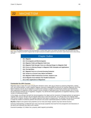
  • 1. 22 MAGNETISM Figure 22.1 The magnificent spectacle of the Aurora Borealis, or northern lights, glows in the northern sky above Bear Lake near Eielson Air Force Base, Alaska. Shaped by the Earth’s magnetic field, this light is produced by radiation spewed from solar storms. (credit: Senior Airman Joshua Strang, via Flickr) Chapter Outline 22.1. Magnets 22.2. Ferromagnets and Electromagnets 22.3. Magnetic Fields and Magnetic Field Lines 22.4. Magnetic Field Strength: Force on a Moving Charge in a Magnetic Field 22.5. Force on a Moving Charge in a Magnetic Field: Examples and Applications 22.6. The Hall Effect 22.7. Magnetic Force on a Current-Carrying Conductor 22.8. Torque on a Current Loop: Motors and Meters 22.9. Magnetic Fields Produced by Currents: Ampere’s Law 22.10. Magnetic Force between Two Parallel Conductors 22.11. More Applications of Magnetism Connection for AP® Courses Magnetism plays a major role in your everyday life. All electric motors, with uses as diverse as powering refrigerators, starting cars, and moving elevators, contain magnets. Magnetic resonance imaging (MRI) has become an important diagnostic tool in the field of medicine, and the use of magnetism to explore brain activity is a subject of contemporary research and development. Other applications of magnetism include computer memory, levitation of high-speed trains, the aurora borealis, and, of course, the first important historical use of magnetism: navigation. You will find all of these applications of magnetism linked by a small number of underlying principles. In this chapter, you will learn that both the internal properties of an object and the movement of charged particles can generate a magnetic field, and you will learn why all magnetic fields have a north and south pole. You will also learn how magnetic fields exert forces on objects, resulting in the magnetic alignment that makes a compass work. You will learn how we use this principle to weigh the smallest of subatomic particles with precision and contain superheated plasma to facilitate nuclear fusion. Big Idea 1 Objects and systems have properties such as mass and charge. Systems may have internal structure. Enduring Understanding 1.E Materials have many macroscopic properties that result from the arrangement and interactions of the atoms and molecules that make up the material. Essential Knowledge 1.E.5 Matter has a property called magnetic permeability. Chapter 22 | Magnetism 965
  • 2. Essential Knowledge 1.E.6 Matter has a property called magnetic dipole moment. Big Idea 2 Fields existing in space can be used to explain interactions. Enduring Understanding 2.D A magnetic field is caused by a magnet or a moving electrically charged object. Magnetic fields observed in nature always seem to be produced either by moving charged objects or by magnetic dipoles or combinations of dipoles and never by single poles. Essential Knowledge 2.D.1 The magnetic field exerts a force on a moving electrically charged object. That magnetic force is perpendicular to the direction of the velocity of the object and to the magnetic field and is proportional to the magnitude of the charge, the magnitude of the velocity, and the magnitude of the magnetic field. It also depends on the angle between the velocity and the magnetic field vectors. Treatment is quantitative for angles of 0°, 90°, or 180° and qualitative for other angles. Essential Knowledge 2.D.2 The magnetic field vectors around a straight wire that carries electric current are tangent to concentric circles centered on that wire. The field has no component toward the current-carrying wire. Essential Knowledge 2.D.3 A magnetic dipole placed in a magnetic field, such as the ones created by a magnet or the Earth, will tend to align with the magnetic field vector. Essential Knowledge 2.D.4 Ferromagnetic materials contain magnetic domains that are themselves magnets. Big Idea 3 The interactions of an object with other objects can be described by forces. Enduring Understanding 3.C At the macroscopic level, forces can be categorized as either long-range (action-at-a-distance) forces or contact forces. Essential Knowledge 3.C.3 A magnetic force results from the interaction of a moving charged object or a magnet with other moving charged objects or another magnet. Big Idea 4 Interactions between systems can result in changes in those systems. Enduring Understanding 4.E The electric and magnetic properties of a system can change in response to the presence of, or changes in, other objects or systems. Essential Knowledge 4.E.1 The magnetic properties of some materials can be affected by magnetic fields at the system. Students should focus on the underlying concepts and not the use of the vocabulary. Figure 22.2 Engineering of technology like iPods would not be possible without a deep understanding of magnetism. (credit: Jesse! S?, Flickr) 22.1 Magnets Learning Objectives By the end of this section, you will be able to: • Describe the difference between the north and south poles of a magnet. • Describe how magnetic poles interact with each other. 966 Chapter 22 | Magnetism This content is available for free at http://cnx.org/content/col11844/1.13
  • 3. Figure 22.3 Magnets come in various shapes, sizes, and strengths. All have both a north pole and a south pole. There is never an isolated pole (a monopole). All magnets attract iron, such as that in a refrigerator door. However, magnets may attract or repel other magnets. Experimentation shows that all magnets have two poles. If freely suspended, one pole will point toward the north. The two poles are thus named the north magnetic pole and the south magnetic pole (or more properly, north-seeking and south-seeking poles, for the attractions in those directions). Universal Characteristics of Magnets and Magnetic Poles It is a universal characteristic of all magnets that like poles repel and unlike poles attract. (Note the similarity with electrostatics: unlike charges attract and like charges repel.) Further experimentation shows that it is impossible to separate north and south poles in the manner that + and − charges can be separated. Figure 22.4 One end of a bar magnet is suspended from a thread that points toward north. The magnet’s two poles are labeled N and S for north- seeking and south-seeking poles, respectively. Misconception Alert: Earth’s Geographic North Pole Hides an S The Earth acts like a very large bar magnet with its south-seeking pole near the geographic North Pole. That is why the north pole of your compass is attracted toward the geographic north pole of the Earth—because the magnetic pole that is near the geographic North Pole is actually a south magnetic pole! Confusion arises because the geographic term “North Pole” has come to be used (incorrectly) for the magnetic pole that is near the North Pole. Thus, “North magnetic pole” is actually a misnomer—it should be called the South magnetic pole. Chapter 22 | Magnetism 967
  • 4. Figure 22.5 Unlike poles attract, whereas like poles repel. Figure 22.6 North and south poles always occur in pairs. Attempts to separate them result in more pairs of poles. If we continue to split the magnet, we will eventually get down to an iron atom with a north pole and a south pole—these, too, cannot be separated. Real World Connections: Dipoles and Monopoles Figure 22.6 shows that no matter how many times you divide a magnet the resulting objects are always magnetic dipoles. Formally, a magnetic dipole is an object (usually very small) with a north and south magnetic pole. Magnetic dipoles have a vector property called magnetic momentum. The magnitude of this vector is equal to the strength of its poles and the distance between the poles, and the direction points from the south pole to the north pole. A magnetic dipole can also be thought of as a very small closed current loop. There is no way to isolate north and south magnetic poles like you can isolate positive and negative charges. Another way of saying this is that magnetic fields of a magnetic object always make closed loops, starting at a north pole and ending at a south pole. With a positive charge, you might imagine drawing a spherical surface enclosing that charge, and there would be a net flux of electric field lines flowing outward through that surface. In fact, Gauss’s law states that the electric flux through a surface is proportional to the amount of charge enclosed. With a magnetic object, every surface you can imagine that encloses all or part of the magnet ultimately has zero net flux of magnetic field lines flowing through the surface. Just as many outward-flowing lines from the north pole of the magnet pass through the surface as inward-flowing lines from the south pole of the magnet. Some physicists have theorized that magnetic monopoles exist. These would be isolated magnetic “charges” that would only generate field lines that flow outward or inward (not loops). Despite many searches, we have yet to experimentally verify the existence of magnetic monopoles. 968 Chapter 22 | Magnetism This content is available for free at http://cnx.org/content/col11844/1.13
  • 5. The fact that magnetic poles always occur in pairs of north and south is true from the very large scale—for example, sunspots always occur in pairs that are north and south magnetic poles—all the way down to the very small scale. Magnetic atoms have both a north pole and a south pole, as do many types of subatomic particles, such as electrons, protons, and neutrons. Making Connections: Take-Home Experiment—Refrigerator Magnets We know that like magnetic poles repel and unlike poles attract. See if you can show this for two refrigerator magnets. Will the magnets stick if you turn them over? Why do they stick to the door anyway? What can you say about the magnetic properties of the door next to the magnet? Do refrigerator magnets stick to metal or plastic spoons? Do they stick to all types of metal? 22.2 Ferromagnets and Electromagnets Learning Objectives By the end of this section, you will be able to: • Define ferromagnet. • Describe the role of magnetic domains in magnetization. • Explain the significance of the Curie temperature. • Describe the relationship between electricity and magnetism. The information presented in this section supports the following AP® learning objectives and science practices: • 2.D.3.1 The student is able to describe the orientation of a magnetic dipole placed in a magnetic field in general and the particular cases of a compass in the magnetic field of the Earth and iron filings surrounding a bar magnet. (S.P. 1.2) • 2.D.4.1 The student is able to use the representation of magnetic domains to qualitatively analyze the magnetic behavior of a bar magnet composed of ferromagnetic material. (S.P. 1.4) • 4.E.1.1 The student is able to use representations and models to qualitatively describe the magnetic properties of some materials that can be affected by magnetic properties of other objects in the system. (S.P. 1.1, 1.4, 2.2) Ferromagnets Only certain materials, such as iron, cobalt, nickel, and gadolinium, exhibit strong magnetic effects. Such materials are called ferromagnetic, after the Latin word for iron, ferrum. A group of materials made from the alloys of the rare earth elements are also used as strong and permanent magnets; a popular one is neodymium. Other materials exhibit weak magnetic effects, which are detectable only with sensitive instruments. Not only do ferromagnetic materials respond strongly to magnets (the way iron is attracted to magnets), they can also be magnetized themselves—that is, they can be induced to be magnetic or made into permanent magnets. Figure 22.7 An unmagnetized piece of iron is placed between two magnets, heated, and then cooled, or simply tapped when cold. The iron becomes a permanent magnet with the poles aligned as shown: its south pole is adjacent to the north pole of the original magnet, and its north pole is adjacent to the south pole of the original magnet. Note that there are attractive forces between the magnets. When a magnet is brought near a previously unmagnetized ferromagnetic material, it causes local magnetization of the material with unlike poles closest, as in Figure 22.7. (This results in the attraction of the previously unmagnetized material to the magnet.) What happens on a microscopic scale is illustrated in Figure 22.8. The regions within the material called domains act like small bar magnets. Within domains, the poles of individual atoms are aligned. Each atom acts like a tiny bar magnet. Domains are small and randomly oriented in an unmagnetized ferromagnetic object. In response to an external magnetic field, the domains may grow to millimeter size, aligning themselves as shown in Figure 22.8(b). This induced magnetization can be made permanent if the material is heated and then cooled, or simply tapped in the presence of other magnets. Chapter 22 | Magnetism 969
  • 6. Figure 22.8 (a) An unmagnetized piece of iron (or other ferromagnetic material) has randomly oriented domains. (b) When magnetized by an external field, the domains show greater alignment, and some grow at the expense of others. Individual atoms are aligned within domains; each atom acts like a tiny bar magnet. Conversely, a permanent magnet can be demagnetized by hard blows or by heating it in the absence of another magnet. Increased thermal motion at higher temperature can disrupt and randomize the orientation and the size of the domains. There is a well-defined temperature for ferromagnetic materials, which is called the Curie temperature, above which they cannot be magnetized. The Curie temperature for iron is 1043 K (770ºC) , which is well above room temperature. There are several elements and alloys that have Curie temperatures much lower than room temperature and are ferromagnetic only below those temperatures. Electromagnets Early in the 19th century, it was discovered that electrical currents cause magnetic effects. The first significant observation was by the Danish scientist Hans Christian Oersted (1777–1851), who found that a compass needle was deflected by a current- carrying wire. This was the first significant evidence that the movement of charges had any connection with magnets. Electromagnetism is the use of electric current to make magnets. These temporarily induced magnets are called electromagnets. Electromagnets are employed for everything from a wrecking yard crane that lifts scrapped cars to controlling the beam of a 90-km-circumference particle accelerator to the magnets in medical imaging machines (See Figure 22.9). Figure 22.9 Instrument for magnetic resonance imaging (MRI). The device uses a superconducting cylindrical coil for the main magnetic field. The patient goes into this “tunnel” on the gurney. (credit: Bill McChesney, Flickr) Figure 22.10 shows that the response of iron filings to a current-carrying coil and to a permanent bar magnet. The patterns are similar. In fact, electromagnets and ferromagnets have the same basic characteristics—for example, they have north and south poles that cannot be separated and for which like poles repel and unlike poles attract. 970 Chapter 22 | Magnetism This content is available for free at http://cnx.org/content/col11844/1.13
  • 7. Figure 22.10 Iron filings near (a) a current-carrying coil and (b) a magnet act like tiny compass needles, showing the shape of their fields. Their response to a current-carrying coil and a permanent magnet is seen to be very similar, especially near the ends of the coil and the magnet. Making Connections: Compasses Figure 22.11 Compass needles and a bar magnet. In Figure 22.11, a series of tiny compass needles are placed in an external magnetic field. These dipoles respond exactly like the iron filings in Figure 22.10. For needles close to one pole of the magnet, the needle is aligned so that the opposite pole of the needle points at the bar magnet. For example, close to the north pole of the bar magnet, the south pole of the compass needle is aligned to be closest to the bar magnet. As an experimenter moves each compass around, the needle will rotate in such a way as to orient itself with the field of the bar magnet at that location. In this way, the magnetic field lines may be mapped out precisely. The strength of the magnetic field depends on the medium in which the magnetic field exists. Some substances (like iron) respond to external magnetic fields in a way that amplifies the external magnetic field. The magnetic permeability of a substance is a measure of the substance’s ability to support or amplify an already existing external magnetic field. Ferromagnets, in which magnetic domains in the substance align with and amplify an external magnetic field, are examples of objects with high permeability. Combining a ferromagnet with an electromagnet can produce particularly strong magnetic effects. (See Figure 22.12.) Whenever strong magnetic effects are needed, such as lifting scrap metal, or in particle accelerators, electromagnets are enhanced by ferromagnetic materials. Limits to how strong the magnets can be made are imposed by coil resistance (it will overheat and melt at sufficiently high current), and so superconducting magnets may be employed. These are still limited, because superconducting properties are destroyed by too great a magnetic field. Chapter 22 | Magnetism 971
  • 8. Figure 22.12 An electromagnet with a ferromagnetic core can produce very strong magnetic effects. Alignment of domains in the core produces a magnet, the poles of which are aligned with the electromagnet. Figure 22.13 shows a few uses of combinations of electromagnets and ferromagnets. Ferromagnetic materials can act as memory devices, because the orientation of the magnetic fields of small domains can be reversed or erased. Magnetic information storage on videotapes and computer hard drives are among the most common applications. This property is vital in our digital world. Figure 22.13 An electromagnet induces regions of permanent magnetism on a floppy disk coated with a ferromagnetic material. The information stored here is digital (a region is either magnetic or not); in other applications, it can be analog (with a varying strength), such as on audiotapes. Current: The Source of All Magnetism An electromagnet creates magnetism with an electric current. In later sections we explore this more quantitatively, finding the strength and direction of magnetic fields created by various currents. But what about ferromagnets? Figure 22.14 shows models of how electric currents create magnetism at the submicroscopic level. (Note that we cannot directly observe the paths of individual electrons about atoms, and so a model or visual image, consistent with all direct observations, is made. We can directly observe the electron’s orbital angular momentum, its spin momentum, and subsequent magnetic moments, all of which are explained with electric-current-creating subatomic magnetism.) Currents, including those associated with other submicroscopic particles like protons, allow us to explain ferromagnetism and all other magnetic effects. Ferromagnetism, for example, results from an internal cooperative alignment of electron spins, possible in some materials but not in others. Crucial to the statement that electric current is the source of all magnetism is the fact that it is impossible to separate north and south magnetic poles. (This is far different from the case of positive and negative charges, which are easily separated.) A current loop always produces a magnetic dipole—that is, a magnetic field that acts like a north pole and south pole pair. Since isolated north and south magnetic poles, called magnetic monopoles, are not observed, currents are used to explain all magnetic effects. If magnetic monopoles did exist, then we would have to modify this underlying connection that all magnetism is due to electrical current. There is no known reason that magnetic monopoles should not exist—they are simply never observed—and so 972 Chapter 22 | Magnetism This content is available for free at http://cnx.org/content/col11844/1.13
  • 9. searches at the subnuclear level continue. If they do not exist, we would like to find out why not. If they do exist, we would like to see evidence of them. Electric Currents and Magnetism Electric current is the source of all magnetism. Figure 22.14 (a) In the planetary model of the atom, an electron orbits a nucleus, forming a closed-current loop and producing a magnetic field with a north pole and a south pole. (b) Electrons have spin and can be crudely pictured as rotating charge, forming a current that produces a magnetic field with a north pole and a south pole. Neither the planetary model nor the image of a spinning electron is completely consistent with modern physics. However, they do provide a useful way of understanding phenomena. PhET Explorations: Magnets and Electromagnets Explore the interactions between a compass and bar magnet. Discover how you can use a battery and wire to make a magnet! Can you make it a stronger magnet? Can you make the magnetic field reverse? Figure 22.15 Magnets and Electromagnets (http://cnx.org/content/m55375/1.2/magnets-and-electromagnets_en.jar) 22.3 Magnetic Fields and Magnetic Field Lines Learning Objectives By the end of this section, you will be able to: • Define magnetic field and describe the magnetic field lines of various magnetic fields. Einstein is said to have been fascinated by a compass as a child, perhaps musing on how the needle felt a force without direct physical contact. His ability to think deeply and clearly about action at a distance, particularly for gravitational, electric, and magnetic forces, later enabled him to create his revolutionary theory of relativity. Since magnetic forces act at a distance, we define a magnetic field to represent magnetic forces. The pictorial representation of magnetic field lines is very useful in visualizing the strength and direction of the magnetic field. As shown in Figure 22.16, the direction of magnetic field lines is defined to be the direction in which the north end of a compass needle points. The magnetic field is traditionally called the B- field. Chapter 22 | Magnetism 973
  • 10. Figure 22.16 Magnetic field lines are defined to have the direction that a small compass points when placed at a location. (a) If small compasses are used to map the magnetic field around a bar magnet, they will point in the directions shown: away from the north pole of the magnet, toward the south pole of the magnet. (Recall that the Earth’s north magnetic pole is really a south pole in terms of definitions of poles on a bar magnet.) (b) Connecting the arrows gives continuous magnetic field lines. The strength of the field is proportional to the closeness (or density) of the lines. (c) If the interior of the magnet could be probed, the field lines would be found to form continuous closed loops. Small compasses used to test a magnetic field will not disturb it. (This is analogous to the way we tested electric fields with a small test charge. In both cases, the fields represent only the object creating them and not the probe testing them.) Figure 22.17 shows how the magnetic field appears for a current loop and a long straight wire, as could be explored with small compasses. A small compass placed in these fields will align itself parallel to the field line at its location, with its north pole pointing in the direction of B. Note the symbols used for field into and out of the paper. Figure 22.17 Small compasses could be used to map the fields shown here. (a) The magnetic field of a circular current loop is similar to that of a bar magnet. (b) A long and straight wire creates a field with magnetic field lines forming circular loops. (c) When the wire is in the plane of the paper, the field is perpendicular to the paper. Note that the symbols used for the field pointing inward (like the tail of an arrow) and the field pointing outward (like the tip of an arrow). Making Connections: Concept of a Field A field is a way of mapping forces surrounding any object that can act on another object at a distance without apparent physical connection. The field represents the object generating it. Gravitational fields map gravitational forces, electric fields map electrical forces, and magnetic fields map magnetic forces. Extensive exploration of magnetic fields has revealed a number of hard-and-fast rules. We use magnetic field lines to represent the field (the lines are a pictorial tool, not a physical entity in and of themselves). The properties of magnetic field lines can be summarized by these rules: 1. The direction of the magnetic field is tangent to the field line at any point in space. A small compass will point in the direction of the field line. 2. The strength of the field is proportional to the closeness of the lines. It is exactly proportional to the number of lines per unit area perpendicular to the lines (called the areal density). 3. Magnetic field lines can never cross, meaning that the field is unique at any point in space. 4. Magnetic field lines are continuous, forming closed loops without beginning or end. They go from the north pole to the south pole. The last property is related to the fact that the north and south poles cannot be separated. It is a distinct difference from electric field lines, which begin and end on the positive and negative charges. If magnetic monopoles existed, then magnetic field lines would begin and end on them. 974 Chapter 22 | Magnetism This content is available for free at http://cnx.org/content/col11844/1.13
  • 11. 22.4 Magnetic Field Strength: Force on a Moving Charge in a Magnetic Field Learning Objectives By the end of this section, you will be able to: • Describe the effects of magnetic fields on moving charges. • Use the right-hand rule 1 to determine the velocity of a charge, the direction of the magnetic field, and the direction of magnetic force on a moving charge. • Calculate the magnetic force on a moving charge. The information presented in this section supports the following AP® learning objectives and science practices: • 2.D.1.1 The student is able to apply mathematical routines to express the force exerted on a moving charged object by a magnetic field. (S.P. 2.2) • 3.C.3.1 The student is able to use right-hand rules to analyze a situation involving a current-carrying conductor and a moving electrically charged object to determine the direction of the magnetic force exerted on the charged object due to the magnetic field created by the current-carrying conductor. (S.P. 1.4) What is the mechanism by which one magnet exerts a force on another? The answer is related to the fact that all magnetism is caused by current, the flow of charge. Magnetic fields exert forces on moving charges, and so they exert forces on other magnets, all of which have moving charges. Right Hand Rule 1 The magnetic force on a moving charge is one of the most fundamental known. Magnetic force is as important as the electrostatic or Coulomb force. Yet the magnetic force is more complex, in both the number of factors that affects it and in its direction, than the relatively simple Coulomb force. The magnitude of the magnetic force F on a charge q moving at a speed v in a magnetic field of strength B is given by (22.1)F = qvB sin θ, where θ is the angle between the directions of v and B. This force is often called the Lorentz force. In fact, this is how we define the magnetic field strength B —in terms of the force on a charged particle moving in a magnetic field. The SI unit for magnetic field strength B is called the tesla (T) after the eccentric but brilliant inventor Nikola Tesla (1856–1943). To determine how the tesla relates to other SI units, we solve F = qvB sin θ for B . (22.2) B = F qv sin θ Because sin θ is unitless, the tesla is (22.3) 1 T = 1 N C ⋅ m/s = 1 N A ⋅ m (note that C/s = A). Another smaller unit, called the gauss (G), where 1 G = 10−4 T , is sometimes used. The strongest permanent magnets have fields near 2 T; superconducting electromagnets may attain 10 T or more. The Earth’s magnetic field on its surface is only about 5×10⁻⁵ T , or 0.5 G. The direction of the magnetic force F is perpendicular to the plane formed by v and B , as determined by the right hand rule 1 (or RHR-1), which is illustrated in Figure 22.18. RHR-1 states that, to determine the direction of the magnetic force on a positive moving charge, you point the thumb of the right hand in the direction of v , the fingers in the direction of B , and a perpendicular to the palm points in the direction of F . One way to remember this is that there is one velocity, and so the thumb represents it. There are many field lines, and so the fingers represent them. The force is in the direction you would push with your palm. The force on a negative charge is in exactly the opposite direction to that on a positive charge. Chapter 22 | Magnetism 975
  • 12. Figure 22.18 Magnetic fields exert forces on moving charges. This force is one of the most basic known. The direction of the magnetic force on a moving charge is perpendicular to the plane formed by v and B and follows right hand rule–1 (RHR-1) as shown. The magnitude of the force is proportional to q , v , B , and the sine of the angle between v and B . Making Connections: Charges and Magnets There is no magnetic force on static charges. However, there is a magnetic force on moving charges. When charges are stationary, their electric fields do not affect magnets. But, when charges move, they produce magnetic fields that exert forces on other magnets. When there is relative motion, a connection between electric and magnetic fields emerges—each affects the other. Example 22.1 Calculating Magnetic Force: Earth’s Magnetic Field on a Charged Glass Rod With the exception of compasses, you seldom see or personally experience forces due to the Earth’s small magnetic field. To illustrate this, suppose that in a physics lab you rub a glass rod with silk, placing a 20-nC positive charge on it. Calculate the force on the rod due to the Earth’s magnetic field, if you throw it with a horizontal velocity of 10 m/s due west in a place where the Earth’s field is due north parallel to the ground. (The direction of the force is determined with right hand rule 1 as shown in Figure 22.19.) Figure 22.19 A positively charged object moving due west in a region where the Earth’s magnetic field is due north experiences a force that is straight down as shown. A negative charge moving in the same direction would feel a force straight up. Strategy 976 Chapter 22 | Magnetism This content is available for free at http://cnx.org/content/col11844/1.13
  • 13. We are given the charge, its velocity, and the magnetic field strength and direction. We can thus use the equation F = qvB sin θ to find the force. Solution The magnetic force is (22.4)F = qvb sin θ. We see that sin θ = 1 , since the angle between the velocity and the direction of the field is 90º . Entering the other given quantities yields (22.5)F = ⎛ ⎝20×10–9 C⎞ ⎠(10 m/s)⎛ ⎝5×10⁻⁵ T⎞ ⎠ = 1×10–11 (C ⋅ m/s) ⎛ ⎝ N C ⋅ m/s ⎞ ⎠ = 1×10–11 N. Discussion This force is completely negligible on any macroscopic object, consistent with experience. (It is calculated to only one digit, since the Earth’s field varies with location and is given to only one digit.) The Earth’s magnetic field, however, does produce very important effects, particularly on submicroscopic particles. Some of these are explored in Force on a Moving Charge in a Magnetic Field: Examples and Applications. 22.5 Force on a Moving Charge in a Magnetic Field: Examples and Applications Learning Objectives By the end of this section, you will be able to: • Describe the effects of a magnetic field on a moving charge. • Calculate the radius of curvature of the path of a charge that is moving in a magnetic field. The information presented in this section supports the following AP® learning objectives and science practices: • 3.C.3.1 The student is able to use right-hand rules to analyze a situation involving a current-carrying conductor and a moving electrically charged object to determine the direction of the magnetic force exerted on the charged object due to the magnetic field created by the current-carrying conductor. (S.P. 1.4) Magnetic force can cause a charged particle to move in a circular or spiral path. Cosmic rays are energetic charged particles in outer space, some of which approach the Earth. They can be forced into spiral paths by the Earth’s magnetic field. Protons in giant accelerators are kept in a circular path by magnetic force. The bubble chamber photograph in Figure 22.20 shows charged particles moving in such curved paths. The curved paths of charged particles in magnetic fields are the basis of a number of phenomena and can even be used analytically, such as in a mass spectrometer. Figure 22.20 Trails of bubbles are produced by high-energy charged particles moving through the superheated liquid hydrogen in this artist’s rendition of a bubble chamber. There is a strong magnetic field perpendicular to the page that causes the curved paths of the particles. The radius of the path can be used to find the mass, charge, and energy of the particle. So does the magnetic force cause circular motion? Magnetic force is always perpendicular to velocity, so that it does no work on the charged particle. The particle’s kinetic energy and speed thus remain constant. The direction of motion is affected, but not the speed. This is typical of uniform circular motion. The simplest case occurs when a charged particle moves perpendicular to a Chapter 22 | Magnetism 977
  • 14. uniform B -field, such as shown in Figure 22.21. (If this takes place in a vacuum, the magnetic field is the dominant factor determining the motion.) Here, the magnetic force supplies the centripetal force Fc = mv2 / r . Noting that sin θ = 1 , we see that F = qvB . Figure 22.21 A negatively charged particle moves in the plane of the page in a region where the magnetic field is perpendicular into the page (represented by the small circles with x’s—like the tails of arrows). The magnetic force is perpendicular to the velocity, and so velocity changes in direction but not magnitude. Uniform circular motion results. Because the magnetic force F supplies the centripetal force Fc , we have (22.6) qvB = mv2 r . Solving for r yields (22.7)r = mv qB . Here, r is the radius of curvature of the path of a charged particle with mass m and charge q , moving at a speed v perpendicular to a magnetic field of strength B . If the velocity is not perpendicular to the magnetic field, then v is the component of the velocity perpendicular to the field. The component of the velocity parallel to the field is unaffected, since the magnetic force is zero for motion parallel to the field. This produces a spiral motion rather than a circular one. Example 22.2 Calculating the Curvature of the Path of an Electron Moving in a Magnetic Field: A Magnet on a TV Screen A magnet brought near an old-fashioned TV screen such as in Figure 22.22 (TV sets with cathode ray tubes instead of LCD screens) severely distorts its picture by altering the path of the electrons that make its phosphors glow. (Don’t try this at home, as it will permanently magnetize and ruin the TV.) To illustrate this, calculate the radius of curvature of the path of an electron having a velocity of 6.00×10⁷ m/s (corresponding to the accelerating voltage of about 10.0 kV used in some TVs) perpendicular to a magnetic field of strength B = 0.500 T (obtainable with permanent magnets). 978 Chapter 22 | Magnetism This content is available for free at http://cnx.org/content/col11844/1.13
  • 15. Figure 22.22 Side view showing what happens when a magnet comes in contact with a computer monitor or TV screen. Electrons moving toward the screen spiral about magnetic field lines, maintaining the component of their velocity parallel to the field lines. This distorts the image on the screen. Strategy We can find the radius of curvature r directly from the equation r = mv qB , since all other quantities in it are given or known. Solution Using known values for the mass and charge of an electron, along with the given values of v and B gives us (22.8) r = mv qB = ⎛ ⎝9.11×10⁻³¹ kg⎞ ⎠ ⎛ ⎝6.00×10⁷ m/s⎞ ⎠ ⎛ ⎝1.60×10⁻¹⁹ C⎞ ⎠(0.500 T) = 6.83×10⁻⁴ m or (22.9)r = 0.683 mm. Discussion The small radius indicates a large effect. The electrons in the TV picture tube are made to move in very tight circles, greatly altering their paths and distorting the image. Figure 22.23 shows how electrons not moving perpendicular to magnetic field lines follow the field lines. The component of velocity parallel to the lines is unaffected, and so the charges spiral along the field lines. If field strength increases in the direction of motion, the field will exert a force to slow the charges, forming a kind of magnetic mirror, as shown below. Figure 22.23 When a charged particle moves along a magnetic field line into a region where the field becomes stronger, the particle experiences a force that reduces the component of velocity parallel to the field. This force slows the motion along the field line and here reverses it, forming a “magnetic mirror.” The properties of charged particles in magnetic fields are related to such different things as the Aurora Australis or Aurora Borealis and particle accelerators. Charged particles approaching magnetic field lines may get trapped in spiral orbits about the lines rather than crossing them, as seen above. Some cosmic rays, for example, follow the Earth’s magnetic field lines, entering the atmosphere near the magnetic poles and causing the southern or northern lights through their ionization of molecules in the Chapter 22 | Magnetism 979
  • 16. atmosphere. This glow of energized atoms and molecules is seen in Figure 22.1. Those particles that approach middle latitudes must cross magnetic field lines, and many are prevented from penetrating the atmosphere. Cosmic rays are a component of background radiation; consequently, they give a higher radiation dose at the poles than at the equator. Figure 22.24 Energetic electrons and protons, components of cosmic rays, from the Sun and deep outer space often follow the Earth’s magnetic field lines rather than cross them. (Recall that the Earth’s north magnetic pole is really a south pole in terms of a bar magnet.) Some incoming charged particles become trapped in the Earth’s magnetic field, forming two belts above the atmosphere known as the Van Allen radiation belts after the discoverer James A. Van Allen, an American astrophysicist. (See Figure 22.25.) Particles trapped in these belts form radiation fields (similar to nuclear radiation) so intense that manned space flights avoid them and satellites with sensitive electronics are kept out of them. In the few minutes it took lunar missions to cross the Van Allen radiation belts, astronauts received radiation doses more than twice the allowed annual exposure for radiation workers. Other planets have similar belts, especially those having strong magnetic fields like Jupiter. Figure 22.25 The Van Allen radiation belts are two regions in which energetic charged particles are trapped in the Earth’s magnetic field. One belt lies about 300 km above the Earth’s surface, the other about 16,000 km. Charged particles in these belts migrate along magnetic field lines and are partially reflected away from the poles by the stronger fields there. The charged particles that enter the atmosphere are replenished by the Sun and sources in deep outer space. Back on Earth, we have devices that employ magnetic fields to contain charged particles. Among them are the giant particle accelerators that have been used to explore the substructure of matter. (See Figure 22.26.) Magnetic fields not only control the direction of the charged particles, they also are used to focus particles into beams and overcome the repulsion of like charges in these beams. 980 Chapter 22 | Magnetism This content is available for free at http://cnx.org/content/col11844/1.13
  • 17. Figure 22.26 The Fermilab facility in Illinois has a large particle accelerator (the most powerful in the world until 2008) that employs magnetic fields (magnets seen here in orange) to contain and direct its beam. This and other accelerators have been in use for several decades and have allowed us to discover some of the laws underlying all matter. (credit: ammcrim, Flickr) Thermonuclear fusion (like that occurring in the Sun) is a hope for a future clean energy source. One of the most promising devices is the tokamak, which uses magnetic fields to contain (or trap) and direct the reactive charged particles. (See Figure 22.27.) Less exotic, but more immediately practical, amplifiers in microwave ovens use a magnetic field to contain oscillating electrons. These oscillating electrons generate the microwaves sent into the oven. Figure 22.27 Tokamaks such as the one shown in the figure are being studied with the goal of economical production of energy by nuclear fusion. Magnetic fields in the doughnut-shaped device contain and direct the reactive charged particles. (credit: David Mellis, Flickr) Mass spectrometers have a variety of designs, and many use magnetic fields to measure mass. The curvature of a charged particle’s path in the field is related to its mass and is measured to obtain mass information. (See More Applications of Magnetism.) Historically, such techniques were employed in the first direct observations of electron charge and mass. Today, mass spectrometers (sometimes coupled with gas chromatographs) are used to determine the make-up and sequencing of large biological molecules. 22.6 The Hall Effect Learning Objectives By the end of this section, you will be able to: • Describe the Hall effect. • Calculate the Hall emf across a current-carrying conductor. The information presented in this section supports the following AP® learning objectives and science practices: • 3.C.3.1 The student is able to use right-hand rules to analyze a situation involving a current-carrying conductor and a moving electrically charged object to determine the direction of the magnetic force exerted on the charged object due to the magnetic field created by the current-carrying conductor. (S.P. 1.4) Chapter 22 | Magnetism 981
  • 18. We have seen effects of a magnetic field on free-moving charges. The magnetic field also affects charges moving in a conductor. One result is the Hall effect, which has important implications and applications. Figure 22.28 shows what happens to charges moving through a conductor in a magnetic field. The field is perpendicular to the electron drift velocity and to the width of the conductor. Note that conventional current is to the right in both parts of the figure. In part (a), electrons carry the current and move to the left. In part (b), positive charges carry the current and move to the right. Moving electrons feel a magnetic force toward one side of the conductor, leaving a net positive charge on the other side. This separation of charge creates a voltage ε , known as the Hall emf, across the conductor. The creation of a voltage across a current-carrying conductor by a magnetic field is known as the Hall effect, after Edwin Hall, the American physicist who discovered it in 1879. Figure 22.28 The Hall effect. (a) Electrons move to the left in this flat conductor (conventional current to the right). The magnetic field is directly out of the page, represented by circled dots; it exerts a force on the moving charges, causing a voltage ε , the Hall emf, across the conductor. (b) Positive charges moving to the right (conventional current also to the right) are moved to the side, producing a Hall emf of the opposite sign, –ε . Thus, if the direction of the field and current are known, the sign of the charge carriers can be determined from the Hall effect. One very important use of the Hall effect is to determine whether positive or negative charges carries the current. Note that in Figure 22.28(b), where positive charges carry the current, the Hall emf has the sign opposite to when negative charges carry the current. Historically, the Hall effect was used to show that electrons carry current in metals and it also shows that positive charges carry current in some semiconductors. The Hall effect is used today as a research tool to probe the movement of charges, their drift velocities and densities, and so on, in materials. In 1980, it was discovered that the Hall effect is quantized, an example of quantum behavior in a macroscopic object. The Hall effect has other uses that range from the determination of blood flow rate to precision measurement of magnetic field strength. To examine these quantitatively, we need an expression for the Hall emf, ε , across a conductor. Consider the balance of forces on a moving charge in a situation where B , v , and l are mutually perpendicular, such as shown in Figure 22.29. Although the magnetic force moves negative charges to one side, they cannot build up without limit. The electric field caused by their separation opposes the magnetic force, F = qvB , and the electric force, Fe = qE , eventually grows to equal it. That is, (22.10)qE = qvB or (22.11)E = vB. Note that the electric field E is uniform across the conductor because the magnetic field B is uniform, as is the conductor. For a uniform electric field, the relationship between electric field and voltage is E = ε / l , where l is the width of the conductor and ε is the Hall emf. Entering this into the last expression gives (22.12)ε l = vB. Solving this for the Hall emf yields (22.13)ε = Blv (B, v, and l, mutually perpendicular), where ε is the Hall effect voltage across a conductor of width l through which charges move at a speed v . 982 Chapter 22 | Magnetism This content is available for free at http://cnx.org/content/col11844/1.13
  • 19. Figure 22.29 The Hall emf ε produces an electric force that balances the magnetic force on the moving charges. The magnetic force produces charge separation, which builds up until it is balanced by the electric force, an equilibrium that is quickly reached. One of the most common uses of the Hall effect is in the measurement of magnetic field strength B . Such devices, called Hall probes, can be made very small, allowing fine position mapping. Hall probes can also be made very accurate, usually accomplished by careful calibration. Another application of the Hall effect is to measure fluid flow in any fluid that has free charges (most do). (See Figure 22.30.) A magnetic field applied perpendicular to the flow direction produces a Hall emf ε as shown. Note that the sign of ε depends not on the sign of the charges, but only on the directions of B and v . The magnitude of the Hall emf is ε = Blv , where l is the pipe diameter, so that the average velocity v can be determined from ε providing the other factors are known. Figure 22.30 The Hall effect can be used to measure fluid flow in any fluid having free charges, such as blood. The Hall emf ε is measured across the tube perpendicular to the applied magnetic field and is proportional to the average velocity v . Example 22.3 Calculating the Hall emf: Hall Effect for Blood Flow A Hall effect flow probe is placed on an artery, applying a 0.100-T magnetic field across it, in a setup similar to that in Figure 22.30. What is the Hall emf, given the vessel’s inside diameter is 4.00 mm and the average blood velocity is 20.0 cm/s? Strategy Because B , v , and l are mutually perpendicular, the equation ε = Blv can be used to find ε . Solution Entering the given values for B , v , and l gives (22.14)ε = Blv = (0.100 T)⎛ ⎝4.00×10⁻³ m⎞ ⎠(0.200 m/s) = 80.0 μV Chapter 22 | Magnetism 983
  • 20. Discussion This is the average voltage output. Instantaneous voltage varies with pulsating blood flow. The voltage is small in this type of measurement. ε is particularly difficult to measure, because there are voltages associated with heart action (ECG voltages) that are on the order of millivolts. In practice, this difficulty is overcome by applying an AC magnetic field, so that the Hall emf is AC with the same frequency. An amplifier can be very selective in picking out only the appropriate frequency, eliminating signals and noise at other frequencies. 22.7 Magnetic Force on a Current-Carrying Conductor Learning Objectives By the end of this section, you will be able to: • Describe the effects of a magnetic force on a current-carrying conductor. • Calculate the magnetic force on a current-carrying conductor. The information presented in this section supports the following AP® learning objectives and science practices: • 3.C.3.1 The student is able to use right-hand rules to analyze a situation involving a current-carrying conductor and a moving electrically charged object to determine the direction of the magnetic force exerted on the charged object due to the magnetic field created by the current-carrying conductor. (S.P. 1.4) Because charges ordinarily cannot escape a conductor, the magnetic force on charges moving in a conductor is transmitted to the conductor itself. Figure 22.31 The magnetic field exerts a force on a current-carrying wire in a direction given by the right hand rule 1 (the same direction as that on the individual moving charges). This force can easily be large enough to move the wire, since typical currents consist of very large numbers of moving charges. We can derive an expression for the magnetic force on a current by taking a sum of the magnetic forces on individual charges. (The forces add because they are in the same direction.) The force on an individual charge moving at the drift velocity vd is given by F = qvdB sin θ . Taking B to be uniform over a length of wire l and zero elsewhere, the total magnetic force on the wire is then F = (qvdB sin θ)(N) , where N is the number of charge carriers in the section of wire of length l . Now, N = nV , where n is the number of charge carriers per unit volume and V is the volume of wire in the field. Noting that V = Al , where A is the cross-sectional area of the wire, then the force on the wire is F = (qvdB sin θ)(nAl) . Gathering terms, (22.15)F = (nqAvd)lB sin θ. Because nqAvd = I (see Current), (22.16)F = IlB sin θ is the equation for magnetic force on a length l of wire carrying a current I in a uniform magnetic field B , as shown in Figure 22.32. If we divide both sides of this expression by l , we find that the magnetic force per unit length of wire in a uniform field is F l = IB sin θ . The direction of this force is given by RHR-1, with the thumb in the direction of the current I . Then, with the fingers in the direction of B , a perpendicular to the palm points in the direction of F , as in Figure 22.32. 984 Chapter 22 | Magnetism This content is available for free at http://cnx.org/content/col11844/1.13
  • 21. Figure 22.32 The force on a current-carrying wire in a magnetic field is F = IlB sin θ . Its direction is given by RHR-1. Example 22.4 Calculating Magnetic Force on a Current-Carrying Wire: A Strong Magnetic Field Calculate the force on the wire shown in Figure 22.31, given B = 1.50 T , l = 5.00 cm , and I = 20.0 A . Strategy The force can be found with the given information by using F = IlB sin θ and noting that the angle θ between I and B is 90º , so that sin θ = 1 . Solution Entering the given values into F = IlB sin θ yields (22.17)F = IlB sin θ = (20.0 A)(0.0500 m)(1.50 T)(1). The units for tesla are 1 T = N A ⋅ m ; thus, (22.18)F = 1.50 N. Discussion This large magnetic field creates a significant force on a small length of wire. Magnetic force on current-carrying conductors is used to convert electric energy to work. (Motors are a prime example—they employ loops of wire and are considered in the next section.) Magnetohydrodynamics (MHD) is the technical name given to a clever application where magnetic force pumps fluids without moving mechanical parts. (See Figure 22.33.) Figure 22.33 Magnetohydrodynamics. The magnetic force on the current passed through this fluid can be used as a nonmechanical pump. A strong magnetic field is applied across a tube and a current is passed through the fluid at right angles to the field, resulting in a force on the fluid parallel to the tube axis as shown. The absence of moving parts makes this attractive for moving a hot, chemically active substance, such as the liquid sodium employed in some nuclear reactors. Experimental artificial hearts are Chapter 22 | Magnetism 985
  • 22. testing with this technique for pumping blood, perhaps circumventing the adverse effects of mechanical pumps. (Cell membranes, however, are affected by the large fields needed in MHD, delaying its practical application in humans.) MHD propulsion for nuclear submarines has been proposed, because it could be considerably quieter than conventional propeller drives. The deterrent value of nuclear submarines is based on their ability to hide and survive a first or second nuclear strike. As we slowly disassemble our nuclear weapons arsenals, the submarine branch will be the last to be decommissioned because of this ability (See Figure 22.34.) Existing MHD drives are heavy and inefficient—much development work is needed. Figure 22.34 An MHD propulsion system in a nuclear submarine could produce significantly less turbulence than propellers and allow it to run more silently. The development of a silent drive submarine was dramatized in the book and the film The Hunt for Red October. 22.8 Torque on a Current Loop: Motors and Meters Learning Objectives By the end of this section, you will be able to: • Describe how motors and meters work in terms of torque on a current loop. • Calculate the torque on a current-carrying loop in a magnetic field. Motors are the most common application of magnetic force on current-carrying wires. Motors have loops of wire in a magnetic field. When current is passed through the loops, the magnetic field exerts torque on the loops, which rotates a shaft. Electrical energy is converted to mechanical work in the process. (See Figure 22.35.) Figure 22.35 Torque on a current loop. A current-carrying loop of wire attached to a vertically rotating shaft feels magnetic forces that produce a clockwise torque as viewed from above. Let us examine the force on each segment of the loop in Figure 22.35 to find the torques produced about the axis of the vertical shaft. (This will lead to a useful equation for the torque on the loop.) We take the magnetic field to be uniform over the rectangular loop, which has width w and height l . First, we note that the forces on the top and bottom segments are vertical and, therefore, parallel to the shaft, producing no torque. Those vertical forces are equal in magnitude and opposite in direction, so that they also produce no net force on the loop. Figure 22.36 shows views of the loop from above. Torque is defined as τ = rF sin θ , where F is the force, r is the distance from the pivot that the force is applied, and θ is the angle between r and F . As seen in Figure 22.36(a), right hand rule 1 gives the forces on the sides to be equal in magnitude and opposite in 986 Chapter 22 | Magnetism This content is available for free at http://cnx.org/content/col11844/1.13
  • 23. direction, so that the net force is again zero. However, each force produces a clockwise torque. Since r = w / 2 , the torque on each vertical segment is (w / 2)F sin θ , and the two add to give a total torque. (22.19)τ = w 2 F sin θ + w 2 F sin θ = wF sin θ Figure 22.36 Top views of a current-carrying loop in a magnetic field. (a) The equation for torque is derived using this view. Note that the perpendicular to the loop makes an angle θ with the field that is the same as the angle between w / 2 and F . (b) The maximum torque occurs when θ is a right angle and sin θ = 1 . (c) Zero (minimum) torque occurs when θ is zero and sin θ = 0 . (d) The torque reverses once the loop rotates past θ = 0 . Now, each vertical segment has a length l that is perpendicular to B , so that the force on each is F = IlB . Entering F into the expression for torque yields (22.20)τ = wIlB sin θ. If we have a multiple loop of N turns, we get N times the torque of one loop. Finally, note that the area of the loop is A = wl ; the expression for the torque becomes (22.21)τ = NIAB sin θ. This is the torque on a current-carrying loop in a uniform magnetic field. This equation can be shown to be valid for a loop of any shape. The loop carries a current I , has N turns, each of area A , and the perpendicular to the loop makes an angle θ with the field B . The net force on the loop is zero. Example 22.5 Calculating Torque on a Current-Carrying Loop in a Strong Magnetic Field Find the maximum torque on a 100-turn square loop of a wire of 10.0 cm on a side that carries 15.0 A of current in a 2.00-T field. Chapter 22 | Magnetism 987
  • 24. Strategy Torque on the loop can be found using τ = NIAB sin θ . Maximum torque occurs when θ = 90º and sin θ = 1 . Solution For sin θ = 1 , the maximum torque is (22.22)τmax = NIAB. Entering known values yields (22.23)τmax = (100)(15.0 A)⎛ ⎝0.100 m2⎞ ⎠(2.00 T) = 30.0 N ⋅ m. Discussion This torque is large enough to be useful in a motor. The torque found in the preceding example is the maximum. As the coil rotates, the torque decreases to zero at θ = 0 . The torque then reverses its direction once the coil rotates past θ = 0 . (See Figure 22.36(d).) This means that, unless we do something, the coil will oscillate back and forth about equilibrium at θ = 0 . To get the coil to continue rotating in the same direction, we can reverse the current as it passes through θ = 0 with automatic switches called brushes. (See Figure 22.37.) Figure 22.37 (a) As the angular momentum of the coil carries it through θ = 0 , the brushes reverse the current to keep the torque clockwise. (b) The coil will rotate continuously in the clockwise direction, with the current reversing each half revolution to maintain the clockwise torque. Meters, such as those in analog fuel gauges on a car, are another common application of magnetic torque on a current-carrying loop. Figure 22.38 shows that a meter is very similar in construction to a motor. The meter in the figure has its magnets shaped to limit the effect of θ by making B perpendicular to the loop over a large angular range. Thus the torque is proportional to I and not θ . A linear spring exerts a counter-torque that balances the current-produced torque. This makes the needle deflection proportional to I . If an exact proportionality cannot be achieved, the gauge reading can be calibrated. To produce a galvanometer for use in analog voltmeters and ammeters that have a low resistance and respond to small currents, we use a large loop area A , high magnetic field B , and low-resistance coils. 988 Chapter 22 | Magnetism This content is available for free at http://cnx.org/content/col11844/1.13
  • 25. Figure 22.38 Meters are very similar to motors but only rotate through a part of a revolution. The magnetic poles of this meter are shaped to keep the component of B perpendicular to the loop constant, so that the torque does not depend on θ and the deflection against the return spring is proportional only to the current I . 22.9 Magnetic Fields Produced by Currents: Ampere’s Law Learning Objectives By the end of this section, you will be able to: • Calculate current that produces a magnetic field. • Use the right-hand rule 2 to determine the direction of current or the direction of magnetic field loops. The information presented in this section supports the following AP® learning objectives and science practices: • 2.D.2.1 The student is able to create a verbal or visual representation of a magnetic field around a long straight wire or a pair of parallel wires. (S.P. 1.1) • 3.C.3.1 The student is able to use right-hand rules to analyze a situation involving a current-carrying conductor and a moving electrically charged object to determine the direction of the magnetic force exerted on the charged object due to the magnetic field created by the current-carrying conductor. (S.P. 1.4) • 3.C.3.2 The student is able to plan a data collection strategy appropriate to an investigation of the direction of the force on a moving electrically charged object caused by a current in a wire in the context of a specific set of equipment and instruments and analyze the resulting data to arrive at a conclusion. (S.P. 4.2, 5.1) How much current is needed to produce a significant magnetic field, perhaps as strong as the Earth’s field? Surveyors will tell you that overhead electric power lines create magnetic fields that interfere with their compass readings. Indeed, when Oersted discovered in 1820 that a current in a wire affected a compass needle, he was not dealing with extremely large currents. How does the shape of wires carrying current affect the shape of the magnetic field created? We noted earlier that a current loop created a magnetic field similar to that of a bar magnet, but what about a straight wire or a toroid (doughnut)? How is the direction of a current-created field related to the direction of the current? Answers to these questions are explored in this section, together with a brief discussion of the law governing the fields created by currents. Magnetic Field Created by a Long Straight Current-Carrying Wire: Right Hand Rule 2 Magnetic fields have both direction and magnitude. As noted before, one way to explore the direction of a magnetic field is with compasses, as shown for a long straight current-carrying wire in Figure 22.39. Hall probes can determine the magnitude of the field. The field around a long straight wire is found to be in circular loops. The right hand rule 2 (RHR-2) emerges from this exploration and is valid for any current segment—point the thumb in the direction of the current, and the fingers curl in the direction of the magnetic field loops created by it. Chapter 22 | Magnetism 989
  • 26. Figure 22.39 (a) Compasses placed near a long straight current-carrying wire indicate that field lines form circular loops centered on the wire. (b) Right hand rule 2 states that, if the right hand thumb points in the direction of the current, the fingers curl in the direction of the field. This rule is consistent with the field mapped for the long straight wire and is valid for any current segment. Making Connections: Notation For a wire oriented perpendicular to the page, if the current in the wire is directed out of the page, the right-hand rule tells us that the magnetic field lines will be oriented in a counterclockwise direction around the wire. If the current in the wire is directed into the page, the magnetic field lines will be oriented in a clockwise direction around the wire. We use ⊙ to indicate that the direction of the current in the wire is out of the page, and ⊗ for the direction into the page. Figure 22.40 Two parallel wires have currents pointing into or out of the page as shown. The direction of the magnetic field in the vicinity of the two wires is shown. The magnetic field strength (magnitude) produced by a long straight current-carrying wire is found by experiment to be (22.24) B = µ0 I 2πr (long straight wire), where I is the current, r is the shortest distance to the wire, and the constant µ0 = 4π× 10−7 T ⋅ m/A is the permeability of free space. (µ0 is one of the basic constants in nature. We will see later that µ0 is related to the speed of light.) Since the wire is very long, the magnitude of the field depends only on distance from the wire r , not on position along the wire. 990 Chapter 22 | Magnetism This content is available for free at http://cnx.org/content/col11844/1.13
  • 27. Example 22.6 Calculating Current that Produces a Magnetic Field Find the current in a long straight wire that would produce a magnetic field twice the strength of the Earth’s at a distance of 5.0 cm from the wire. Strategy The Earth’s field is about 5.0×10⁻⁵ T , and so here B due to the wire is taken to be 1.0×10⁻⁴ T . The equation B = µ0 I 2πr can be used to find I , since all other quantities are known. Solution Solving for I and entering known values gives (22.25) I = 2πrB µ0 = 2π⎛ ⎝5.0×10⁻² m⎞ ⎠ ⎛ ⎝1.0×10⁻⁴ T⎞ ⎠ 4π×10−7 T ⋅ m/A = 25 A. Discussion So a moderately large current produces a significant magnetic field at a distance of 5.0 cm from a long straight wire. Note that the answer is stated to only two digits, since the Earth’s field is specified to only two digits in this example. Ampere’s Law and Others The magnetic field of a long straight wire has more implications than you might at first suspect. Each segment of current produces a magnetic field like that of a long straight wire, and the total field of any shape current is the vector sum of the fields due to each segment. The formal statement of the direction and magnitude of the field due to each segment is called the Biot- Savart law. Integral calculus is needed to sum the field for an arbitrary shape current. This results in a more complete law, called Ampere’s law, which relates magnetic field and current in a general way. Ampere’s law in turn is a part of Maxwell’s equations, which give a complete theory of all electromagnetic phenomena. Considerations of how Maxwell’s equations appear to different observers led to the modern theory of relativity, and the realization that electric and magnetic fields are different manifestations of the same thing. Most of this is beyond the scope of this text in both mathematical level, requiring calculus, and in the amount of space that can be devoted to it. But for the interested student, and particularly for those who continue in physics, engineering, or similar pursuits, delving into these matters further will reveal descriptions of nature that are elegant as well as profound. In this text, we shall keep the general features in mind, such as RHR-2 and the rules for magnetic field lines listed in Magnetic Fields and Magnetic Field Lines, while concentrating on the fields created in certain important situations. Making Connections: Relativity Hearing all we do about Einstein, we sometimes get the impression that he invented relativity out of nothing. On the contrary, one of Einstein’s motivations was to solve difficulties in knowing how different observers see magnetic and electric fields. Magnetic Field Produced by a Current-Carrying Circular Loop The magnetic field near a current-carrying loop of wire is shown in Figure 22.41. Both the direction and the magnitude of the magnetic field produced by a current-carrying loop are complex. RHR-2 can be used to give the direction of the field near the loop, but mapping with compasses and the rules about field lines given in Magnetic Fields and Magnetic Field Lines are needed for more detail. There is a simple formula for the magnetic field strength at the center of a circular loop. It is (22.26) B = µ0 I 2R (at center of loop), where R is the radius of the loop. This equation is very similar to that for a straight wire, but it is valid only at the center of a circular loop of wire. The similarity of the equations does indicate that similar field strength can be obtained at the center of a loop. One way to get a larger field is to have N loops; then, the field is B = Nµ0I / (2R) . Note that the larger the loop, the smaller the field at its center, because the current is farther away. Chapter 22 | Magnetism 991
  • 28. Figure 22.41 (a) RHR-2 gives the direction of the magnetic field inside and outside a current-carrying loop. (b) More detailed mapping with compasses or with a Hall probe completes the picture. The field is similar to that of a bar magnet. Magnetic Field Produced by a Current-Carrying Solenoid A solenoid is a long coil of wire (with many turns or loops, as opposed to a flat loop). Because of its shape, the field inside a solenoid can be very uniform, and also very strong. The field just outside the coils is nearly zero. Figure 22.42 shows how the field looks and how its direction is given by RHR-2. Figure 22.42 (a) Because of its shape, the field inside a solenoid of length l is remarkably uniform in magnitude and direction, as indicated by the straight and uniformly spaced field lines. The field outside the coils is nearly zero. (b) This cutaway shows the magnetic field generated by the current in the solenoid. The magnetic field inside of a current-carrying solenoid is very uniform in direction and magnitude. Only near the ends does it begin to weaken and change direction. The field outside has similar complexities to flat loops and bar magnets, but the magnetic field strength inside a solenoid is simply (22.27)B = µ0nI (inside a solenoid), where n is the number of loops per unit length of the solenoid (n = N / l , with N being the number of loops and l the length). Note that B is the field strength anywhere in the uniform region of the interior and not just at the center. Large uniform fields spread over a large volume are possible with solenoids, as Example 22.7 implies. Example 22.7 Calculating Field Strength inside a Solenoid What is the field inside a 2.00-m-long solenoid that has 2000 loops and carries a 1600-A current? Strategy 992 Chapter 22 | Magnetism This content is available for free at http://cnx.org/content/col11844/1.13
  • 29. To find the field strength inside a solenoid, we use B = µ0nI . First, we note the number of loops per unit length is (22.28) n = N l = 2000 2.00 m = 1000 m−1 = 10 cm−1 . Solution Substituting known values gives (22.29)B = µ0nI = ⎛ ⎝4π×10−7 T ⋅ m/A⎞ ⎠ ⎛ ⎝1000 m−1⎞ ⎠(1600 A) = 2.01 T. Discussion This is a large field strength that could be established over a large-diameter solenoid, such as in medical uses of magnetic resonance imaging (MRI). The very large current is an indication that the fields of this strength are not easily achieved, however. Such a large current through 1000 loops squeezed into a meter’s length would produce significant heating. Higher currents can be achieved by using superconducting wires, although this is expensive. There is an upper limit to the current, since the superconducting state is disrupted by very large magnetic fields. Applying the Science Practices: Charged Particle in a Magnetic Field Visit here (http://openstaxcollege.org/l/31particlemagnetic) and start the simulation applet “Particle in a Magnetic Field (2D)” in order to explore the magnetic force that acts on a charged particle in a magnetic field. Experiment with the simulation to see how it works and what parameters you can change; then construct a plan to methodically investigate how magnetic fields affect charged particles. Some questions you may want to answer as part of your experiment are: • Are the paths of charged particles in magnetic fields always similar in two dimensions? Why or why not? • How would the path of a neutral particle in the magnetic field compare to the path of a charged particle? • How would the path of a positive particle differ from the path of a negative particle in a magnetic field? • What quantities dictate the properties of the particle’s path? • If you were attempting to measure the mass of a charged particle moving through a magnetic field, what would you need to measure about its path? Would you need to see it moving at many different velocities or through different field strengths, or would one trial be sufficient if your measurements were correct? • Would doubling the charge change the path through the field? Predict an answer to this question, and then test your hypothesis. • Would doubling the velocity change the path through the field? Predict an answer to this question, and then test your hypothesis. • Would doubling the magnetic field strength change the path through the field? Predict an answer to this question, and then test your hypothesis. • Would increasing the mass change the path? Predict an answer to this question, and then test your hypothesis. There are interesting variations of the flat coil and solenoid. For example, the toroidal coil used to confine the reactive particles in tokamaks is much like a solenoid bent into a circle. The field inside a toroid is very strong but circular. Charged particles travel in circles, following the field lines, and collide with one another, perhaps inducing fusion. But the charged particles do not cross field lines and escape the toroid. A whole range of coil shapes are used to produce all sorts of magnetic field shapes. Adding ferromagnetic materials produces greater field strengths and can have a significant effect on the shape of the field. Ferromagnetic materials tend to trap magnetic fields (the field lines bend into the ferromagnetic material, leaving weaker fields outside it) and are used as shields for devices that are adversely affected by magnetic fields, including the Earth’s magnetic field. PhET Explorations: Generator Generate electricity with a bar magnet! Discover the physics behind the phenomena by exploring magnets and how you can use them to make a bulb light. Figure 22.43 Generator (http://cnx.org/content/m55399/1.4/generator_en.jar) Chapter 22 | Magnetism 993
  • 30. 22.10 Magnetic Force between Two Parallel Conductors Learning Objectives By the end of this section, you will be able to: • Describe the effects of the magnetic force between two conductors. • Calculate the force between two parallel conductors. The information presented in this section supports the following AP® learning objectives and science practices: • 2.D.2.1 The student is able to create a verbal or visual representation of a magnetic field around a long straight wire or a pair of parallel wires. (S.P. 1.1) • 3.C.3.1 The student is able to use right-hand rules to analyze a situation involving a current-carrying conductor and a moving electrically charged object to determine the direction of the magnetic force exerted on the charged object due to the magnetic field created by the current-carrying conductor. (S.P. 1.4) You might expect that there are significant forces between current-carrying wires, since ordinary currents produce significant magnetic fields and these fields exert significant forces on ordinary currents. But you might not expect that the force between wires is used to define the ampere. It might also surprise you to learn that this force has something to do with why large circuit breakers burn up when they attempt to interrupt large currents. The force between two long straight and parallel conductors separated by a distance r can be found by applying what we have developed in preceding sections. Figure 22.44 shows the wires, their currents, the fields they create, and the subsequent forces they exert on one another. Let us consider the field produced by wire 1 and the force it exerts on wire 2 (call the force F2 ). The field due to I1 at a distance r is given to be (22.30) B1 = µ0 I1 2πr . Figure 22.44 (a) The magnetic field produced by a long straight conductor is perpendicular to a parallel conductor, as indicated by RHR-2. (b) A view from above of the two wires shown in (a), with one magnetic field line shown for each wire. RHR-1 shows that the force between the parallel conductors is attractive when the currents are in the same direction. A similar analysis shows that the force is repulsive between currents in opposite directions. This field is uniform along wire 2 and perpendicular to it, and so the force F2 it exerts on wire 2 is given by F = IlB sin θ with sin θ = 1 : (22.31)F2 = I2lB1. By Newton’s third law, the forces on the wires are equal in magnitude, and so we just write F for the magnitude of F2 . (Note that F1 = −F2 .) Since the wires are very long, it is convenient to think in terms of F / l , the force per unit length. Substituting the expression for B1 into the last equation and rearranging terms gives (22.32)F l = µ0 I1 I2 2πr . F / l is the force per unit length between two parallel currents I1 and I2 separated by a distance r . The force is attractive if the currents are in the same direction and repulsive if they are in opposite directions. 994 Chapter 22 | Magnetism This content is available for free at http://cnx.org/content/col11844/1.13
  • 31. Making Connections: Field Canceling For two parallel wires, the fields will tend to cancel out in the area between the wires. Figure 22.45 Two parallel wires have currents pointing in the same direction, out of the page. The direction of the magnetic fields induced by each wire is shown. Note that the magnetic influence of the wire on the left-hand side extends beyond the wire on the right-hand side. To the right of both wires, the total magnetic field is directed toward the top of the page and is the result of the sum of the fields of both wires. Obviously, the closer wire has a greater effect on the overall magnetic field, but the more distant wire also contributes. One wire cannot block the magnetic field of another wire any more than a massive stone floor beneath you can block the gravitational field of the Earth. Parallel wires with currents in the same direction attract, as you can see if we isolate the magnetic field lines of wire 2 influencing the current in wire 1. Right-hand rule 1 tells us the direction of the resulting magnetic force. Figure 22.46 The same two wires are shown, but now only a part of the magnetic field due to wire 2 is shown in order to demonstrate how the magnetic force from wire 2 affects wire 1. When the currents point in opposite directions as shown, the magnetic field in between the two wires is augmented. In the region outside of the two wires, along the horizontal line connecting the wires, the magnetic fields partially cancel. Figure 22.47 Two wires with parallel currents pointing in opposite directions are shown. The direction of the magnetic field due to each wire is indicated. Parallel wires with currents in opposite directions repel, as you can see if we isolate the magnetic field lines of wire 2 influencing the current in wire 1. Right-hand rule 1 tells us the direction of the resulting magnetic force. Chapter 22 | Magnetism 995
  • 32. Figure 22.48 The same two wires with opposite currents are shown, but now only a part of the magnetic field due to wire 2 is shown in order to demonstrate how the magnetic force from wire 2 affects wire 1. This force is responsible for the pinch effect in electric arcs and plasmas. The force exists whether the currents are in wires or not. In an electric arc, where currents are moving parallel to one another, there is an attraction that squeezes currents into a smaller tube. In large circuit breakers, like those used in neighborhood power distribution systems, the pinch effect can concentrate an arc between plates of a switch trying to break a large current, burn holes, and even ignite the equipment. Another example of the pinch effect is found in the solar plasma, where jets of ionized material, such as solar flares, are shaped by magnetic forces. The operational definition of the ampere is based on the force between current-carrying wires. Note that for parallel wires separated by 1 meter with each carrying 1 ampere, the force per meter is (22.33) F l = ⎛ ⎝4π×10−7 T ⋅ m/A⎞ ⎠(1 A)2 (2π)(1 m) = 2×10⁻⁷ N/m. Since µ0 is exactly 4π×10−7 T ⋅ m/A by definition, and because 1 T = 1 N/(A ⋅ m) , the force per meter is exactly 2×10⁻⁷ N/m . This is the basis of the operational definition of the ampere. The Ampere The official definition of the ampere is: One ampere of current through each of two parallel conductors of infinite length, separated by one meter in empty space free of other magnetic fields, causes a force of exactly 2×10⁻⁷ N/m on each conductor. Infinite-length straight wires are impractical and so, in practice, a current balance is constructed with coils of wire separated by a few centimeters. Force is measured to determine current. This also provides us with a method for measuring the coulomb. We measure the charge that flows for a current of one ampere in one second. That is, 1 C = 1 A ⋅ s . For both the ampere and the coulomb, the method of measuring force between conductors is the most accurate in practice. 22.11 More Applications of Magnetism Learning Objectives By the end of this section, you will be able to: • Describe some applications of magnetism. Mass Spectrometry The curved paths followed by charged particles in magnetic fields can be put to use. A charged particle moving perpendicular to a magnetic field travels in a circular path having a radius r . (22.34)r = mv qB It was noted that this relationship could be used to measure the mass of charged particles such as ions. A mass spectrometer is a device that measures such masses. Most mass spectrometers use magnetic fields for this purpose, although some of them have extremely sophisticated designs. Since there are five variables in the relationship, there are many possibilities. However, if v , q , and B can be fixed, then the radius of the path r is simply proportional to the mass m of the charged particle. Let us examine one such mass spectrometer that has a relatively simple design. (See Figure 22.49.) The process begins with an ion 996 Chapter 22 | Magnetism This content is available for free at http://cnx.org/content/col11844/1.13
  • 33. source, a device like an electron gun. The ion source gives ions their charge, accelerates them to some velocity v , and directs a beam of them into the next stage of the spectrometer. This next region is a velocity selector that only allows particles with a particular value of v to get through. Figure 22.49 This mass spectrometer uses a velocity selector to fix v so that the radius of the path is proportional to mass. The velocity selector has both an electric field and a magnetic field, perpendicular to one another, producing forces in opposite directions on the ions. Only those ions for which the forces balance travel in a straight line into the next region. If the forces balance, then the electric force F = qE equals the magnetic force F = qvB , so that qE = qvB . Noting that q cancels, we see that (22.35) v = E B is the velocity particles must have to make it through the velocity selector, and further, that v can be selected by varying E and B . In the final region, there is only a uniform magnetic field, and so the charged particles move in circular arcs with radii proportional to particle mass. The paths also depend on charge q , but since q is in multiples of electron charges, it is easy to determine and to discriminate between ions in different charge states. Mass spectrometry today is used extensively in chemistry and biology laboratories to identify chemical and biological substances according to their mass-to-charge ratios. In medicine, mass spectrometers are used to measure the concentration of isotopes used as tracers. Usually, biological molecules such as proteins are very large, so they are broken down into smaller fragments before analyzing. Recently, large virus particles have been analyzed as a whole on mass spectrometers. Sometimes a gas chromatograph or high-performance liquid chromatograph provides an initial separation of the large molecules, which are then input into the mass spectrometer. Cathode Ray Tubes—CRTs—and the Like What do non-flat-screen TVs, old computer monitors, x-ray machines, and the 2-mile-long Stanford Linear Accelerator have in common? All of them accelerate electrons, making them different versions of the electron gun. Many of these devices use magnetic fields to steer the accelerated electrons. Figure 22.50 shows the construction of the type of cathode ray tube (CRT) found in some TVs, oscilloscopes, and old computer monitors. Two pairs of coils are used to steer the electrons, one vertically and the other horizontally, to their desired destination. Chapter 22 | Magnetism 997
  • 34. Figure 22.50 The cathode ray tube (CRT) is so named because rays of electrons originate at the cathode in the electron gun. Magnetic coils are used to steer the beam in many CRTs. In this case, the beam is moved down. Another pair of horizontal coils would steer the beam horizontally. Magnetic Resonance Imaging Magnetic resonance imaging (MRI) is one of the most useful and rapidly growing medical imaging tools. It non-invasively produces two-dimensional and three-dimensional images of the body that provide important medical information with none of the hazards of x-rays. MRI is based on an effect called nuclear magnetic resonance (NMR) in which an externally applied magnetic field interacts with the nuclei of certain atoms, particularly those of hydrogen (protons). These nuclei possess their own small magnetic fields, similar to those of electrons and the current loops discussed earlier in this chapter. When placed in an external magnetic field, such nuclei experience a torque that pushes or aligns the nuclei into one of two new energy states—depending on the orientation of its spin (analogous to the N pole and S pole in a bar magnet). Transitions from the lower to higher energy state can be achieved by using an external radio frequency signal to “flip” the orientation of the small magnets. (This is actually a quantum mechanical process. The direction of the nuclear magnetic field is quantized as is energy in the radio waves. We will return to these topics in later chapters.) The specific frequency of the radio waves that are absorbed and reemitted depends sensitively on the type of nucleus, the chemical environment, and the external magnetic field strength. Therefore, this is a resonance phenomenon in which nuclei in a magnetic field act like resonators (analogous to those discussed in the treatment of sound in Oscillatory Motion and Waves) that absorb and reemit only certain frequencies. Hence, the phenomenon is named nuclear magnetic resonance (NMR). NMR has been used for more than 50 years as an analytical tool. It was formulated in 1946 by F. Bloch and E. Purcell, with the 1952 Nobel Prize in Physics going to them for their work. Over the past two decades, NMR has been developed to produce detailed images in a process now called magnetic resonance imaging (MRI), a name coined to avoid the use of the word “nuclear” and the concomitant implication that nuclear radiation is involved. (It is not.) The 2003 Nobel Prize in Medicine went to P. Lauterbur and P. Mansfield for their work with MRI applications. The largest part of the MRI unit is a superconducting magnet that creates a magnetic field, typically between 1 and 2 T in strength, over a relatively large volume. MRI images can be both highly detailed and informative about structures and organ functions. It is helpful that normal and non-normal tissues respond differently for slight changes in the magnetic field. In most medical images, the protons that are hydrogen nuclei are imaged. (About 2/3 of the atoms in the body are hydrogen.) Their location and density give a variety of medically useful information, such as organ function, the condition of tissue (as in the brain), and the shape of structures, such as vertebral disks and knee-joint surfaces. MRI can also be used to follow the movement of certain ions across membranes, yielding information on active transport, osmosis, dialysis, and other phenomena. With excellent spatial resolution, MRI can provide information about tumors, strokes, shoulder injuries, infections, etc. An image requires position information as well as the density of a nuclear type (usually protons). By varying the magnetic field slightly over the volume to be imaged, the resonant frequency of the protons is made to vary with position. Broadcast radio frequencies are swept over an appropriate range and nuclei absorb and reemit them only if the nuclei are in a magnetic field with the correct strength. The imaging receiver gathers information through the body almost point by point, building up a tissue map. The reception of reemitted radio waves as a function of frequency thus gives position information. These “slices” or cross sections through the body are only several mm thick. The intensity of the reemitted radio waves is proportional to the concentration of the nuclear type being flipped, as well as information on the chemical environment in that area of the body. Various techniques are available for enhancing contrast in images and for obtaining more information. Scans called T1, T2, or proton density scans rely on different relaxation mechanisms of nuclei. Relaxation refers to the time it takes for the protons to return to equilibrium after the external field is turned off. This time depends upon tissue type and status (such as inflammation). While MRI images are superior to x rays for certain types of tissue and have none of the hazards of x rays, they do not completely supplant x-ray images. MRI is less effective than x rays for detecting breaks in bone, for example, and in imaging breast tissue, so the two diagnostic tools complement each other. MRI images are also expensive compared to simple x-ray images and tend to be used most often where they supply information not readily obtained from x rays. Another disadvantage of MRI is that the patient is totally enclosed with detectors close to the body for about 30 minutes or more, leading to claustrophobia. It is also difficult for the obese patient to be in the magnet tunnel. New “open-MRI” machines are now available in which the magnet does not completely surround the patient. Over the last decade, the development of much faster scans, called “functional MRI” (fMRI), has allowed us to map the functioning of various regions in the brain responsible for thought and motor control. This technique measures the change in blood flow for activities (thought, experiences, action) in the brain. The nerve cells increase their consumption of oxygen when active. Blood hemoglobin releases oxygen to active nerve cells and has somewhat different magnetic properties when oxygenated than when deoxygenated. With MRI, we can measure this and detect a blood oxygen-dependent signal. Most of the brain scans today use fMRI. 998 Chapter 22 | Magnetism This content is available for free at http://cnx.org/content/col11844/1.13
  • 35. Ampere’s law: B-field: Biot-Savart law: Curie temperature: direction of magnetic field lines: domains: electromagnet: electromagnetism: ferromagnetic: gauss: Hall effect: Hall emf: Lorentz force: magnetic field: Other Medical Uses of Magnetic Fields Currents in nerve cells and the heart create magnetic fields like any other currents. These can be measured but with some difficulty since their strengths are about 10−6 to 10−8 less than the Earth’s magnetic field. Recording of the heart’s magnetic field as it beats is called a magnetocardiogram (MCG), while measurements of the brain’s magnetic field is called a magnetoencephalogram (MEG). Both give information that differs from that obtained by measuring the electric fields of these organs (ECGs and EEGs), but they are not yet of sufficient importance to make these difficult measurements common. In both of these techniques, the sensors do not touch the body. MCG can be used in fetal studies, and is probably more sensitive than echocardiography. MCG also looks at the heart’s electrical activity whose voltage output is too small to be recorded by surface electrodes as in EKG. It has the potential of being a rapid scan for early diagnosis of cardiac ischemia (obstruction of blood flow to the heart) or problems with the fetus. MEG can be used to identify abnormal electrical discharges in the brain that produce weak magnetic signals. Therefore, it looks at brain activity, not just brain structure. It has been used for studies of Alzheimer’s disease and epilepsy. Advances in instrumentation to measure very small magnetic fields have allowed these two techniques to be used more in recent years. What is used is a sensor called a SQUID, for superconducting quantum interference device. This operates at liquid helium temperatures and can measure magnetic fields thousands of times smaller than the Earth’s. Finally, there is a burgeoning market for magnetic cures in which magnets are applied in a variety of ways to the body, from magnetic bracelets to magnetic mattresses. The best that can be said for such practices is that they are apparently harmless, unless the magnets get close to the patient’s computer or magnetic storage disks. Claims are made for a broad spectrum of benefits from cleansing the blood to giving the patient more energy, but clinical studies have not verified these claims, nor is there an identifiable mechanism by which such benefits might occur. PhET Explorations: Magnet and Compass Ever wonder how a compass worked to point you to the Arctic? Explore the interactions between a compass and bar magnet, and then add the Earth and find the surprising answer! Vary the magnet's strength, and see how things change both inside and outside. Use the field meter to measure how the magnetic field changes. Figure 22.51 Magnet and Compass (http://cnx.org/content/m55403/1.2/magnet-and-compass_en.jar) Glossary the physical law that states that the magnetic field around an electric current is proportional to the current; each segment of current produces a magnetic field like that of a long straight wire, and the total field of any shape current is the vector sum of the fields due to each segment another term for magnetic field a physical law that describes the magnetic field generated by an electric current in terms of a specific equation the temperature above which a ferromagnetic material cannot be magnetized the direction that the north end of a compass needle points regions within a material that behave like small bar magnets an object that is temporarily magnetic when an electrical current is passed through it the use of electrical currents to induce magnetism materials, such as iron, cobalt, nickel, and gadolinium, that exhibit strong magnetic effects G, the unit of the magnetic field strength; 1 G = 10–4 T the creation of voltage across a current-carrying conductor by a magnetic field the electromotive force created by a current-carrying conductor by a magnetic field, ε = Blv the force on a charge moving in a magnetic field the representation of magnetic forces Chapter 22 | Magnetism 999
  • 36. magnetic field lines: magnetic field strength (magnitude) produced by a long straight current-carrying wire: magnetic field strength at the center of a circular loop: magnetic field strength inside a solenoid: magnetic force: magnetic monopoles: magnetic resonance imaging (MRI): magnetized: magnetocardiogram (MCG): magnetoencephalogram (MEG): Maxwell’s equations: meter: motor: north magnetic pole: nuclear magnetic resonance (NMR): permeability of free space: right hand rule 1 (RHR-1): right hand rule 2 (RHR-2): solenoid: south magnetic pole: tesla: the pictorial representation of the strength and the direction of a magnetic field defined as B = µ0 I 2πr , where I is the current, r is the shortest distance to the wire, and µ0 is the permeability of free space defined as B = µ0 I 2R where R is the radius of the loop defined as B = µ0nI where n is the number of loops per unit length of the solenoid (n = N / l , with N being the number of loops and l the length) the force on a charge produced by its motion through a magnetic field; the Lorentz force an isolated magnetic pole; a south pole without a north pole, or vice versa (no magnetic monopole has ever been observed) a medical imaging technique that uses magnetic fields create detailed images of internal tissues and organs to be turned into a magnet; to be induced to be magnetic a recording of the heart’s magnetic field as it beats a measurement of the brain’s magnetic field a set of four equations that describe electromagnetic phenomena common application of magnetic torque on a current-carrying loop that is very similar in construction to a motor; by design, the torque is proportional to I and not θ , so the needle deflection is proportional to the current loop of wire in a magnetic field; when current is passed through the loops, the magnetic field exerts torque on the loops, which rotates a shaft; electrical energy is converted to mechanical work in the process the end or the side of a magnet that is attracted toward Earth’s geographic north pole a phenomenon in which an externally applied magnetic field interacts with the nuclei of certain atoms the measure of the ability of a material, in this case free space, to support a magnetic field; the constant µ0 = 4π×10−7 T ⋅ m/A the rule to determine the direction of the magnetic force on a positive moving charge: when the thumb of the right hand points in the direction of the charge’s velocity v and the fingers point in the direction of the magnetic field B , then the force on the charge is perpendicular and away from the palm; the force on a negative charge is perpendicular and into the palm a rule to determine the direction of the magnetic field induced by a current-carrying wire: Point the thumb of the right hand in the direction of current, and the fingers curl in the direction of the magnetic field loops a thin wire wound into a coil that produces a magnetic field when an electric current is passed through it the end or the side of a magnet that is attracted toward Earth’s geographic south pole T, the SI unit of the magnetic field strength; 1 T = 1 N A ⋅ m Section Summary 22.1 Magnets • Magnetism is a subject that includes the properties of magnets, the effect of the magnetic force on moving charges and currents, and the creation of magnetic fields by currents. • There are two types of magnetic poles, called the north magnetic pole and south magnetic pole. • North magnetic poles are those that are attracted toward the Earth’s geographic north pole. • Like poles repel and unlike poles attract. • Magnetic poles always occur in pairs of north and south—it is not possible to isolate north and south poles. 1000 Chapter 22 | Magnetism This content is available for free at http://cnx.org/content/col11844/1.13