2. 2
necessitates consideration of a higher number of targets.
In this study, techniques will therefore be tested on a large
sample of representative UK gauging stations.
Previous studies have focused on either a single
technique or a small number of techniques all belonging
to the same general approach (for instance, regression
techniques: Hirsch, 1982; scaling techniques: Kottegoda and
Elgy, 1977). An unprecedented aspect of this study is the
inclusion of a large number of techniques, spanning a variety
of statistical formulations.
The relative performance of infilling techniques
can be compared through infilling artificially created gaps
(for example, Gyau-Boakye and Schultz, 1994), but this
methodology is highly dependent upon the period in which
the gaps are established. An alternative approach, followed by
this study, is to compare the ability of techniques to simulate
entire target flow records (for example, Elshorbagy et al.,
2000), providing an indication of techniques which can be
expected to perform better for any given gap.
Data and methodology
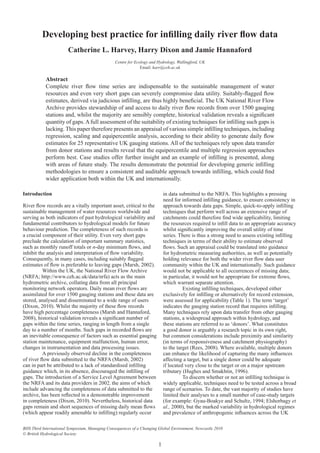
A representative sample of 25 NRFA target stations was
selected from around the UK, incorporating both very
responsive (including urban) and groundwater-fed rivers
(Figure 1). Associated primary and secondary donors were
selected from both nested and neighbouring catchments,
since network density means geographically local donors
are difficult to find in some parts of the country. Donors
were chosen using NRFA catchment and station metadata,
according to factors such as location, base flow index (BFI;
Gustard et al., 1992) and regime similarity (Table 2).
Ten infilling techniques, embracing equipercentile,
scaling and regression approaches, were tested according to
their ability to simulate the target daily mean flow records
(Table 3). Hydrological modelling of target flow series was Figure 1 Map of the UK showing the target station locations by NRFA ID.
Table 1. Existing infilling techniques.
Method Summary Example reference
Manual Gaps are infilled through visual comparison with Rees (2008)
inference donor flows. Accuracy should be fairly assured for
short gaps with no rainfall events, or alternatively
for longer gaps during stable recessions, but other
scenarios would lead to increased difficulty and
subjectivity.
Serial These include linear, polynomial and spline Rees (2008)
interpolation interpolation and are likely to only be successful
techniques throughout stable periods.
Scaling Donor flows are multiplied by a scaling factor, such Kottegoda and Elgy (1977)
factors as the ratio of the donor and target catchment areas
or a weighting based upon the linear distance
between the target and donor.
Equipercentile The percentile value of the donor flow on any given Hughes and Smakhtin
technique day is assumed equal to the percentile value of the (1996)
target flow. Flow gaps are estimated by calculating
the donor flow percentile values and using the
existing target flow data to derive the flow
equivalent to this percentile value at the target.
Linear A regression equation between the target and a Hirsch (1982)
regression donor is derived, commonly via the least squares
method, and used to calculate absent target flows.
Flows may first be transformed, for example, via
the logarithmic transformation.
Hydrological This can vary from black-box modelling, whereby Khalil et al. (2001)
modelling the inputs to the model are related to the outputs
with no consideration of the processes involved, to
the much more complex process-based models and
use of artificial neural networks.
3. 3
Table 2 Target and associated donor stations.
Target River and location Catchment BFI Primary Secondary
station area (km2
) donor donor
NRFA ID
7001 Findhorn at Shenachie 415.6 0.36 7002 7004
15003 Tay at Caputh 3210 0.64 15007 15006
21026 Tima Water at Deephope 31 0.26 21017 21007
25003 Trout Beck at Moor House 11.4 0.14 23009 76014
27071 Swale at Crakehill 1363 0.46 27007 27034
28031 Manifold at Ilam 148.5 0.54 28008 28046
29002 Great Eau at Claythorpe Mill 77.4 0.89 29003 29001
33006 Wissey at Northwold 274.5 0.82 33007 33019
33039 Bedford Ouse at Roxton 1660 0.57 33037 33015
35003 Alde at Farnham 63.9 0.37 35002 35013
38014 Salmon Brook at Edmonton 20.5 0.29 38022 38021
38030 Beane at Hartham 175.1 0.75 38004 33033
39101 Aldbourne at Ramsbury 53.1 0.97 39077 39037
41029 Bull at Lealands 40.8 0.38 41016 41003
43017 West Avon at Upavon 84.6 0.71 53013 53002
46003 Dart at Austins Bridge 247.6 0.52 46005 46008
54029 Teme at Knightsford Bridge 1480 0.54 54008 55014
55029 Monnow at Grosmont 354 0.50 56012 55013
63004 Ystwyth at Pont Llolwyn 169.6 0.40 55008 63001
69017 Goyt at Marple Bridge 183 0.53 69007 69015
74001 Duddon at Duddon Hall 85.7 0.30 74007 74008
76003 Eamont at Udford 396.2 0.52 76004 76015
85004 Luss Water at Luss 35.3 0.28 86001 85003
93001 Carron at New Kelso 137.8 0.26 4005 4006
96002 Naver at Apigill 477 0.42 2002 3002
Table 3 Infilling techniques tested by this study. In order to account for any flow records containing zero flows,
the log-transformation took the form of ln(flow+1). Techniques were applied to datasets comprising days
when observed flows existed for both the target and primary donor (single donor techniques) or all three
stations (dual donor techniques).
Acronym Name Details
LR Linear regression Least-squares linear regression between target and primary donor.
LR Log Linear regression log As above but using log-transformed flows.
M1 MOVE.1 MOVE.1 regression between target and primary donors (Hirsch, 1982).
M1 Log MOVE.1 log As above but using log-transformed flows.
Equi Equipercentile Equipercentile technique applied using percentiles derived
from the primary donor flows.
CA Catchment area scaling Catchment area scaling technique applied using the catchment areas
of the target and primary donor.
LTM Long-term mean Long-term mean scaling technique applied using long-term mean flow
values of the target and primary donor flows.
MR Multiple regression Least-squares linear regression between target and both donors.
MR Log Multiple regression log As above but using log-transformed flows.
W.Equi Weighted Equipercentile technique applied using each of the donor records
equipercentile and taking the average of the resulting estimates for each date.
not considered since, despite its potential to offer highly
accurate estimates, current methods are too resource-intensive
for rapid application to a large number of stations. Model
calibration requirements also constrain portability between
catchments. Simple manual inference and serial interpolation
techniques were also omitted as, despite their undoubted
practical utility, they are heavily reliant upon subjective
decisions and cannot be easily automated and objectively
compared within a testing framework. A final criterion was
to utilise only river flow data, avoiding dependence on other
datasets (in particular, catchment rainfall) which may not
always be readily available to users.
Technique performance was evaluated according
to three commonly used indices, the choice of which was
informed by the recommendations of studies which have
assessed performance indictors (Legates and McCabe, 1999;
Moriasi et al., 2007):
Nash-Sutcliffe Model Efficiency Coefficient (NSE; Nash
and Sutcliffe, 1970):
(1)
Values can range from –∞ to 1, with higher values implying
greater accuracy and values below zero indicating that the
estimated series is less accurate than if the mean of the
observed series had been used. The statistic is widely used
and, as a standardised statistic, has the advantage of being
easily comparable across different catchments.
Root Mean Square Error (RMSE):
(2)
4. 4
Lower values indicate better performance, but comparing
values between different targets is limited since differing
variance between targets is not accounted for.
Percent Bias (PBIAS):
(3)
This index highlights consistent under- or over-estimation
of target flows, which would likely correlate to poorer
performance.
In addition to the above statistics, the means of the
absolute residuals between the observed and estimated flows
were calculated for each target station and compared using
the non-parametric Wilcoxon test, to indicate whether a given
technique generated estimated series with significantly lower
means of residuals than those generated by other techniques.
Results
The overall performance of the techniques is demonstrated
via box plots of the NSE and PBIAS values derived for the
25 series estimated by each technique (Figure 2), whilst their
performance for each individual target is illustrated via bar
plots of the NSE values for each series and technique (Figure
3). The RMSE values indicate analogous results to the NSE
values so the latter was chosen to present results since, as
a standardised statistic, it is easier to compare across the
different targets.
In terms of the NSE value box plots, the interquartile
ranges and bottom whiskers exceed 0.5 for all of the
techniques, albeit to varying degrees. Some techniques have
outlying values which fall below zero, results which are
important for differentiating between how widely applicable
the techniques are. The most favourable techniques are
Figure 2 Box plots of (a) NSE and (b) PBIAS values for the 25 series
estimated by each technique. Whiskers extend to the most
extreme values which are no more than 1.5 multiplied by
the interquartile range away from the box.
Figure 3. Bar plots of NSE values for each target and each technique.
5. 5
the equipercentile and multiple donor techniques, none of
which have outliers falling below 0.5 and all of which have
lower quartile, median and upper quartile values of a higher
magnitude than the other techniques. Not only do these
techniques therefore have wider application, but they also
produce estimated series of greater accuracy.
The PBIAS values are generally of low magnitude
for the majority of techniques, except the CA technique,
which is conspicuous for its heavily biased estimates. Those
techniques based upon log-transformed flows also exhibit
some bias. This can be linked to failure of these techniques to
maintain the mean of the observed series in their estimates.
For some individual targets, the techniques perform
very similarly, although to differing degrees. For example,
all techniques produce NSE values exceeding 0.94 for target
54029 and between 0.72 and 0.82 for target 25003. For
other targets, there is much greater variability in technique
performance (for example, 33039 and 76003), a finding which
is further explored later (see first case study). In certain cases,
the multiple donor techniques offer clear improvement (for
example, stations 33006 and 38014).
There are particular stations for which specific
techniques lead to distinctly lower NSE values, most
prominent of these being M1 Log for targets 46003 and 76003
(see second case study), CA and LTM for targets 35003 and
38030 and CA for targets 27071 and 43017. Overall, CA is a
comparatively poorer technique, having most of the lowest
NSE values associated with it as well as the highest PBIAS
values. Moreover, its NSE values have the lowest lower
quartile, median and upper quartile magnitudes of all the
techniques, in addition to the greatest number of both outliers
and outliers falling below zero.
The results of the Wilcoxon significance testing
(Figure 4) further reinforce the findings so far. The
equipercentile and multiple donor techniques more frequently
produce significantly lower means of residuals than the other
techniques, whilst all of the techniques outperform the CA
technique for the vast majority (in some cases all) of the
targets.
and highlights the value of using a large sample of target
gauging stations. The catchment area scaling technique
essentially seems too simple to capture the influences
affecting the target and even very closely related stations
seldom exhibit a linear relationship with catchment area
(Hughes and Smakhtin, 1996).
In some cases, data transfer from multiple donors
offers an improvement over a single donor, endorsing the
general argument of multiple donors being more capable of
capturing the many influences affecting target flows. In many
other cases, however, the single and multiple techniques yield
sensibly identical performances, such that there is no marked
advantage to including multiple donors. With respect to the
influence of donor choice on technique performance, there
are two clear results. Firstly, for the five targets with NSE
values exceeding 0.9 under all single donor techniques, the
primary donors are either upstream, downstream or nested
compared to the targets and the multiple donor techniques
offer no further improvement in these cases. Secondly, none
of the techniques succeed in producing estimated series with
NSE values exceeding 0.9 when neither donor is upstream,
downstream or nested. This suggests that the relative
locations of the donors could be a critical factor in technique
performance and work is ongoing to investigate this further.
Future work will also interpret the results according to base
flow index, to determine whether a target’s catchment regime
affects technique performance, as well as whether base flow
index is a reliable factor in donor identification.
The general conclusions that can be drawn from the
overall results could contribute to broad infilling guidelines,
but assessing technique performance for individual targets
exposes other areas of discussion. Two case studies are
therefore now presented, the first looking at using localised
data and the second covering technique performance at
different flow magnitudes. An infilling example is also shown.
First case study: Salmon Brook at Edmonton (38014)
The Salmon Brook at Edmonton gauging station (38014)
represents a small, impervious catchment in the south of
the UK. The site originally comprised a compound broad-
crested weir structure, known to be less effective than the
1980 replacement flat V weir (Marsh and Hannaford, 2008).
This change is reflected in a marked quality difference
between the pre-1980 and post-1980 data. Prior to 1980,
the poorer data quality results in an adverse impact on the
relationship between the target and donor flows, confirmed
when comparing the NSE values derived under each of the
techniques for the full datasets to those of the post-1980 data
(Table 4). There is less of an increase in performance for the
multiple donor techniques as, although the primary donor
record extends back to 1954, the secondary donor record only
starts in 1971.
Table 4. Comparison of NSE values for full and post-1980 datasets when
estimating target series 38014.
Technique Full Dataset Post-1980 Dataset
LR 0.813 0.869
LR Log 0.777 0.852
M1 0.804 0.864
M1 Log 0.796 0.861
Equi 0.809 0.863
CA 0.760 0.846
LTM 0.774 0.825
MR 0.955 0.965
MR Log 0.948 0.957
W.Equi 0.955 0.963
Figure 4 Results of significance testing. Values at the intersection of
technique A (y-axis) and technique B (x-axis) indicate the
percentage more (positive values) or less (negative values)
of targets for which A produced significantly lower means of
residuals compared to B (at the 5% level). Values are colour-
coded from red for -100% to green for +100%.
Discussion
Assessing the ability of the chosen infilling techniques to
generate estimated target flow series has revealed certain
techniques to noticeably outperform, or in the case of the
catchment area scaling technique, underperform the other
techniques for specific target stations. This is a key outcome,
since it associates wider applicability to the former techniques
6. 6
This is therefore a clear example of when localising donor
data can be expected to improve the accuracy of estimates
for flow gaps. As well as the replacement or modification
of gauging structures, the homogeneity of UK flow records
has been affected by changes relating to instrumentation,
land use and artificial influences. These may also necessitate
the use of localised data and highlight the need to maintain
comprehensive user guidance information alongside
hydrometric records (Dixon, 2010). Other means of localising
datasets are to consider wet and dry epochs separately
(Hughes and Smakhtin, 1996) or to group flows according
to the month or season that they correspond to, which has
been demonstrated to offer significant improvement (Raman
et al., 1995). Ongoing work by the authors is exploring such
approaches, by applying the same infilling techniques to both
full and localised datasets.
Second case study: Eamont at Udford (76003)
The Eamont at Udford gauging station (76003) in north-
west England gauges a catchment artificially influenced by
storage in lakes and reservoirs. In this case, the single donor
techniques regressing log-transformed flows performed
markedly more poorly than their counterparts regressing
non-transformed flows. As would logically be expected,
however, visual inspection of the estimated series intimates
that log-transforming the flows can yield greater accuracy at
lower flows, despite less accuracy at higher flows. By way
of example, Figure 5 displays all regression-based estimates
for a higher flow period and a lower flow period. The visual
disparity between the MR and MR Log estimates is less
apparent, but RMSEs for LR, M1 and MR are all lower
(higher) during the higher (lower) flow period than those for
LR Log, M1 Log and MR Log.
The RMSEs of the entire estimated series were
calculated separately for lower and higher observed flows
(Table 5). Better performance of regression-based techniques
is evident at higher flows when flows are not transformed,
whereas log-transforming flows gives equivalent or better
performance than non-transforming flows at lower flows.
Lower (higher) flows were simply defined as lower (higher)
than the observed series mean, excluding the lowest (highest)
5% of flows, and varying these groupings could enhance this
distinction. The RMSEs also imply larger residuals for higher
compared to lower flows. The considerable discrepancies
identified by the performance indicators between LR and LR
Figure 5 Estimated and observed flows at target 76003 during a
higher flow (left panel, linear scale) and a lower flow period
(right panel, logarithmic scale).
Table 5 RMSE values of estimates for target station 76003, derived via
regression-based techniques and calculated separately according
to the magnitude of the observed flows.
RMSE
Dataset LR LR Log M1 M1 Log MR MR Log
Lower flows 411.4 318.3 366.6 364.3 132.7 132.2
Higher flows 621.4 794.8 634.8 1070.0 204.9 239
Log and M1 and M1 Log can thus be attributed to squaring
the differences between the observed and estimated values,
which attaches greater weight to larger differences and biases
the indicators towards the better performance of LR and M1
at higher flows.
Ongoing work by the authors is investigating a
novel methodology of grouping estimates according to flow
magnitude and assessing technique performance separately
for each group. This may allow easier identification of
instances when particular techniques surpass others at
certain flow magnitudes and could also isolate favourable
technique combinations. A number of studies has previously
advocated that a single technique is unlikely to be optimal
for all occasions of missing data (for example: Hughes and
Smakhtin, 1996; Gyau-Boakye and Schultz, 1994).
Application example
The South Tyne at Haydon Bridge (23004) is part of the UK
benchmark catchment network, often used within climate
change detection studies (for example: Hannaford and
Marsh, 2008). As such, it is particularly important that its
record be as complete as possible. A nearby upstream station
at Featherstone (23006) is a suitable primary donor, also
representing a natural flow regime of similar responsiveness.
Due to artificial influences acting on other nearby stations,
a secondary donor is more difficult to establish, therefore
an infilling attempt will be made using the equipercentile
technique, concluded as arguably the best of the single donor
techniques.
In 1972, a low flow control was installed at Haydon
Bridge, with low flows prior to this being of limited accuracy
(Marsh and Hannaford, 2008), evident when inspecting the
earlier record. Consequently, a localised target dataset of
post-1971 flows was used. Equipercentile flow estimates
were derived to infill a three-month long gap in the record in
Figure 6 Top: Observed 1972 flows for the South Tyne at Haydon Bridge
(23004) and estimated flows under equipercentile and
CA techniques, based upon donor of South Tyne at Featherstone
(23006). Bottom: Rainfall from the Met Office rain gauge 14284.
7. 7
1972, which reflects the installation of this control (Figure
6). Catchment area estimates were also calculated, to offer
comparison between better and poorer techniques.
This example serves to successfully illustrate the
purpose of this study. It presents a data gap in a flow record
which appears amenable to an infilling attempt, since a good
donor exists and, based on recorded rainfall patterns and
catchment response, the majority of the missing flows could
be expected to be mid-range (estimates for the very low
observed flows at the end of the gap should be treated with
more caution as these infilling techniques are not suggested
for estimating extreme low or high flows). A simple infilling
technique is then applied, producing reliable infill estimates.
The results of this study are also reflected, in that the
equipercentile estimates clearly suggest greater accuracy than
the CA estimates.
Conclusion
Complete flow records are a vitally important resource but
difficult to attain, given the many ways in which data gaps
can arise. Simple infilling techniques that can be rapidly
deployed across large numbers of records would find
wide applicability and be highly beneficial in improving
consistency and confidence in the approach towards reducing
data gaps.
This study has assessed ten techniques, all relying
on single or multiple donor station data transfer, according
to their ability to generate estimated flow series for 25
representative UK target stations. Key findings concern the
importance of the geographical locations of donor stations
relative to target stations and the overall better performance
of the equipercentile and multiple donor techniques versus
the overall poorer performance of the catchment area scaling
technique. The aim of this study has not, however, been to
pinpoint a single optimal technique, but to investigate the
ranges of applicability of each of the techniques. Testing
a large sample of stations has thus allowed identification
of cases where there are notable discrepancies between
technique performances, highlighting the wider applicability
of certain techniques.
More detailed work is underway to examine issues
such as the influence of donor station choice, the potential for
techniques to perform differently at varying flow magnitudes
and the improvement that localising datasets could offer.
Case-by-case analysis will allow interpretation of results
according to the different catchment characteristics and
flow regimes of the target stations. Future work will also
explore more applications of infilling, to further examine the
practicalities of implementing the key findings of this study.
Backed by the support of national archives,
hydrometric measuring agencies are often best placed to
derive realistic flow estimates for data gaps, given their
detailed knowledge of gauging stations. Within the UK,
the findings of this study and future work will allow the
development of general infilling guidance appropriate to
the wide range of flow regimes that exist and embracing a
range of techniques, with local hydrological conditions and
the hydrometric experience of measuring agencies guiding
the method choice and application. It is hoped that this
research will therefore help initiate systematic infilling of
contemporary flow data which, coupled with clear flagging
of estimates, will greatly improve the utility of flow series
to end users. Moreover, consistent infilling methodologies
will facilitate retrospective improvement of key national flow
records, through the infilling of gaps, correction of erroneous
periods and reviewing existing estimates within historical data.
Outside the sphere of operational hydrometry, the
adoption of a consistent and tested approach to river flow
data infilling offers many potential benefits to scientists and
practitioners, both within the UK and more widely. Finally,
it must be emphasised that the ability of simple infilling
techniques to generate reliable infill estimates, as illustrated
by the infilling example presented within this study, does not
replace the need to maximise the quality and completeness of
observed data.
Acknowledgements
The authors would like to thank their colleague Terry Marsh
at the Centre for Ecology and Hydrology for his assistance
with this study. All data was sourced from the National River
Flow Archive.
References
Dixon, H. 2010. Managing national hydrometric data: from
data to information. In: Global Change – Facing Risks and
Threats to Water Resources (Proceedings of the Sixth World
FRIEND Conference, Fez, Morocco, October 2010). IAHS
Publication no. 340. In Press.
Elshorbagy, A.A., Panu, U.S. and Simonovic, S.P. 2000.
Group-based estimation of missing hydrological data: II.
Application to streamflows. Hydrolog. Sci. J., 45, 867–880.
Gustard, A., Bullock, A. and Dixon, J.M. 1992. Low flow
estimation in the United Kingdom. Institute of Hydrology
Report No. 108.
Gyau-Boakye, P. and Schultz, G.A. 1994. Filling gaps in
runoff time-series in West-Africa. Hydrolog. Sci. J., 39,
621–636.
Hannaford, J. and Marsh, T.J. 2008. High-flow and flood
trends in a network of undisturbed catchments in the UK.
Int. J. Climatol., 28, 1325–1338.
Hirsch, R.M. 1982. A comparison of four streamflow record
extension techniques. Water Resour. Res., 15, 1781–1790.
Hughes, D.A. and Smakhtin, V. 1996. Daily flow time series
patching or extension: A spatial interpolation approach
based on flow duration curves. Hydrolog. Sci. J., 41,
851–871.
Khalil, M., Panu, U.S. and Lennox, W.C. 2001. Groups and
neural networks based streamflow data infilling procedures.
J. Hydrol., 241, 153–176.
Kottegoda, N.T. and Elgy, J. 1977. Infilling missing flow
data. In: Morel-Seytoux, H.J. (ed). Modelling Hydrologic
Processes. Water Resources Publications.
Legates, D.R. and McCabe Jr, G.J. 1999. Evaluating the
use of “goodness-of-fit” measures in hydrologic and
hydroclimatic model validation. Water Resour. Res., 35,
233–241.
Marsh, T.J. 2002. Capitalising on river flow data to meet
changing national needs - a UK perspective. Flow
Measurement and Instrumentation, 13, 291-298.
Marsh, T.J. and Hannaford, J. (Eds). 2008. UK Hydrometric
Register. Hydrological data UK series. Centre for Ecology
& Hydrology.
Moriasi, D.N., Arnold, J.G., Van Liew, M.W., Bingner, R.L.,
Harmel, R.D. and Veith, T.L. 2007. Model evaluation
guidelines for systematic quantification of accuracy in
watershed simulations. Trans. ASABE, 50, 885–900.
Nash, J.E. and Sutcliffe, J.V. 1970. River flow forecasting
through conceptual models. Part 1: A discussion of
principles. J. Hydrol., 10, 282-290.
8. 8
Raman, H., Mohan, S. and Padalinathan, P. 1995. Models for
extending streamflow data: a case study. Hydrolog. Sci., 40,
381–393.
Rees, G. 2008. Hydrological data. In: Gustard, A. and
Demuth, S. (eds). Manual on Low-flow Estimation and
Prediction. Operational Hydrology Report No. 50. World
Meteorological Organisation.