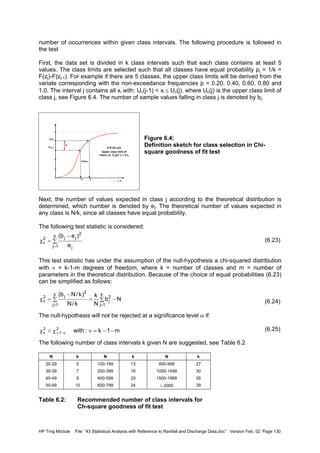
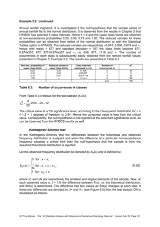
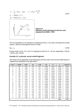
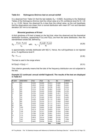
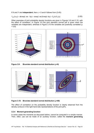
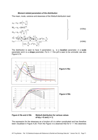
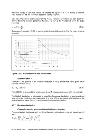
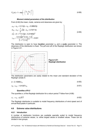
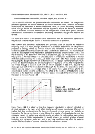
This document provides guidance on statistical analysis of rainfall and discharge data. It discusses graphical representation of data including histograms, line diagrams, and cumulative frequency diagrams. It also covers measures of central tendency, dispersion, skewness, kurtosis and percentiles. The document emphasizes that hydrological time series must meet stationarity conditions to be suitable for statistical analysis and discusses evaluating and accounting for trends and periodic components when analyzing rainfall and discharge data.


![HP Trng Module File: “43 Statistical Analysis with Reference to Rainfall and Discharge Data.doc” Version Feb. 02 Page 25
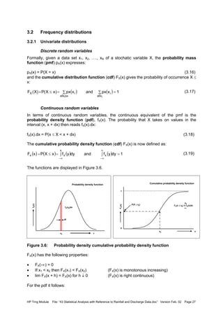
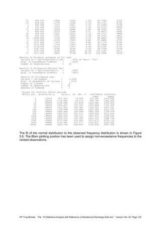
(2) Call event A = wet day 1 after a dry day and event B = wet day 2 after a dry day. Now
we require again P(A∩B) = P(B|A) . P(A). The probability of a wet day after a dry day
is P(A) = 0.17 and the probability of a wet day given that the previous day was also
wet = P(B|A) = 0.34. Hence, P(A∩B) = P(B|A). P(A) = 0.34 . 0.17 = 0.06. This
probability is seen to be about half the probability of having two dry days in a row
after a dry day. This is due to the fact that for Balasinor the probability of having a
wet day followed by a dry day or vice versa is about half the probability of having two
wet or two dry days sequentially.
Example 3.4 Prior and posterior probabilities, using Bayes rule
In a basin for a considerable period of time rainfall was measured using a dense network.
Based on these values for the month July the following classification is used for the basin
rainfall.
Class Rainfall (mm) Probability
Dry
Moderate
Wet
Extremely wet
P < 50
50 ≤ P < 200
200 ≤ P < 400
P ≥ 400
P[A1] = 0.15
P[A2] = 0.50
P[A3] = 0.30
P[A4] = 0.05
Table 3.2: Rainfall classes and probability.
The probabilities presented in Table 3.2 refer to prior probabilities. Furthermore, from the
historical record it has been deduced that the percentage of gauges, which gave a rainfall
amount in a certain class given that the basin rainfall felt in a certain class is given in Table
3.3.
Percentage of gaugesBasin rainfall
P < 50 50 ≤ P < 200 200 ≤ P < 400 P ≥ 400
P < 50
50 ≤ P < 200
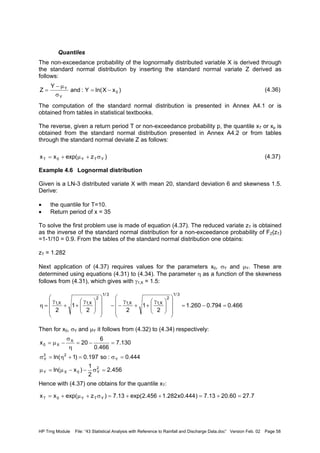
200 ≤ P < 400
P ≥ 400
80
25
5
0
15
65
20
10
5
8
60
25
0
2
15
65
Table 3.3: Conditional probabilities for gauge value given the basin rainfall
Note that the conditional probabilities in the rows add up to 100%.
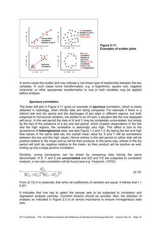
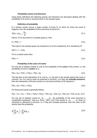
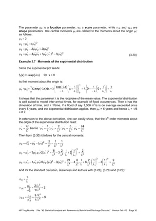
For a particular year a gauge gives a rainfall amount for July of 230 mm. Given that sample
value of 230 mm, what is the class of the basin rainfall in July for that year.
Note that the point rainfall falls in class III. The posterior probability of the actual basin
rainfall in July of that year becomes:
The denominator becomes:
The denominator expresses the probability of getting sample 1 when the prior probabilities
are as given in Table 3.2, which is of course very low.
∑
=
= 4
1i
ii
ii
i
]].P[AA|1P[sample
]].P[AA|1P[sample
1]sample|P[A
0.2950.15x0.050.60x0.300.20x0.500.05x0.15]A|[sample1
4
1i
i =+++=∑
=](https://image.slidesharecdn.com/download-manuals-hydrometeorology-dataprocessing-43statisticalanalysiswithreftorainfall-140512060654-phpapp01/85/Download-manuals-hydrometeorology-data-processing-43statisticalanalysiswithreftorainfall-35-320.jpg)
![HP Trng Module File: “43 Statistical Analysis with Reference to Rainfall and Discharge Data.doc” Version Feb. 02 Page 26
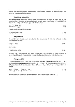
Hence,
Note that the sum of posterior probabilities adds up to 1.
Now, for the same month in the same year from another gauge a rainfall of 280 mm is
obtained. Based on this second sample the posterior probability of the actual July basin
rainfall in that particular year can be obtained by using the above posterior probabilities as
revised prior probabilities for the July rainfall:
Note that the denominator has increased from 0.240 to 0.478.
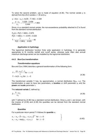
Again note that the posterior probabilities add up to 1. From the above it is seen how the
probability on the state of July rainfall changes with the two sample values:
Class Prior probability After sample 1 After sample 2
I
II
III
IV
0.15
0.50
0.30
0.05
0.025
0.340
0.610
0.025
0.003
0.155
0.834
0.008
Table 3.4: Updating of state probabilities by sampling
Given the two samples, the probability that the rainfall in July for that year is of class III has
increased from 0.30 to 0.834.
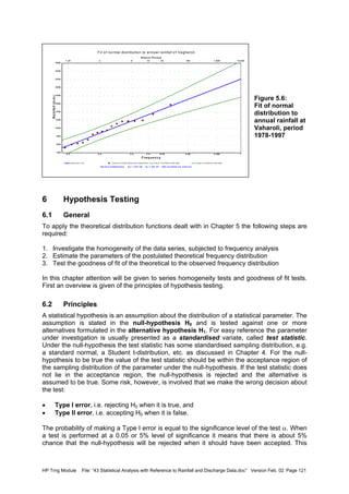
Question: What will be the change in the last column of Table 3.4 if the third sample
gives a value of 180 mm?
0.025
0.295
0.15x0.05
sample1]|P[A
0.610
0.295
0.60x0.30
sample1]|P[A
0.340
0.295
0.20x0.50
sample1]|P[A
0.025
0.295
0.05x0.15
sample1]|P[A
4
3
2
1
==
==
==
==
∑
=
=+++=
4
1i
i 0.4390.15x0.0250.60x0.6100.20x0.3400.05x0.025]A|2[sample
0.008
0.439
0.15x0.025
2]sample|P[A
0.834
0.439
0.60x0.610
2]sample|P[A
0.155
0.439
0.20x0.340
2]sample|P[A
0.003
0.439
0.05x0.025
2]sample|P[A
4
3
2
1
==
==
==
==](https://image.slidesharecdn.com/download-manuals-hydrometeorology-dataprocessing-43statisticalanalysiswithreftorainfall-140512060654-phpapp01/85/Download-manuals-hydrometeorology-data-processing-43statisticalanalysiswithreftorainfall-36-320.jpg)

![HP Trng Module File: “43 Statistical Analysis with Reference to Rainfall and Discharge Data.doc” Version Feb. 02 Page 29
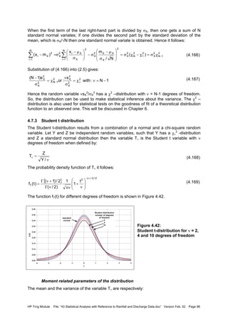
(3.21)
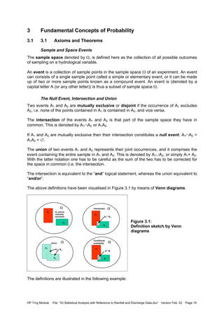
Note that in the above the notation for the quantile xT or x(T) is used. Others use the notation
xp for quantile where p = Fx(xp), i.e. non-exceedance probability.
Mathematical expectation
If X is any continuous random variable with pdf fX(x), and if g(X) is any real-valued function,
defined for all real x for which fX(x) is not zero, then the mathematical expectation of the
function g(X) reads:
(3.22)
Moments
If one chooses g(X) = Xk
, where k = 1, 2, …. Then the kth
moment of X about the origin is
defined by:
(3.23)
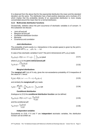
Note that an (‘) is used to indicate moments about the origin. Of special interest is the first
moment about the origin, i.e. the mean:
(3.24)
If instead of the origin, the moment is taken around the mean, then the central moment
follows (µk). Note that the accent (‘) is omitted here to denote a central moment. The second
central moment is the variance:
(3.25)
With the above one defines:
• the standard deviation σX, which expresses the spread around the mean in the same
dimension as the original variate:
(3.26)
• the coefficient of variation Cv:
(3.27)
• the skewness coefficient γ1,x of the distribution is defined by:
(3.28)
• the peakedness of the distribution, expressed by the kurtosis γ2,X:
(3.29)
[ ] ∫=
+∞
∞−
(x)dxg(x)fg(X)E X
[ ] ∫==µ
+∞
∞−
(x)dxfxXE X
kk'
k
[ ] ( )∫==µ=µ′
+∞
∞−
dxxxfXE xx1
[ ][ ] [ ] ∫ µ−=µ−=−==µ
+∞
∞−
(x)dxf)(x)(XE)XE(XEVar(X) X
2
X
2
X
2
2
2X Var(X) µ==σ
X
X
'
1
2
vC
µ
σ
=
µ
µ
=
∫
+∞
∞−
µ−
σ
=
σ
µ
=γ (x)dxf)(x
1
X
3
X3
X
3
X
3
X1,
∫
+∞
∞−
µ−
σ
=
σ
µ
=γ (x)dxf)(x
1
X
4
X4
X
4
X
4
X2,
)(xF1
1
)xP(X1
1
)xP(X
1
T
TXTT −
=
≤−
=
>
=](https://image.slidesharecdn.com/download-manuals-hydrometeorology-dataprocessing-43statisticalanalysiswithreftorainfall-140512060654-phpapp01/85/Download-manuals-hydrometeorology-data-processing-43statisticalanalysiswithreftorainfall-39-320.jpg)
![HP Trng Module File: “43 Statistical Analysis with Reference to Rainfall and Discharge Data.doc” Version Feb. 02 Page 32
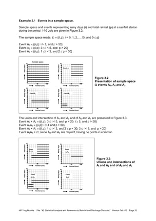
(3.37)
and similarly for the density function:
(3.38)
Moments
In addition to the moments for univariate distributions the moments for bivariate distributions
are defined as follows:
(3.39)
Covariance and correlation function
Of special interest is the central moment expressing the linear dependency between X and
Y, i.e. the covariance:
(3.40)
Note that if X is independent of Y, then with (3.38) it follows:
(3.41)
As discussed in Chapter 2, a standardised representation of the covariance is given by the
correlation coefficient ρXY:
(3.42)
In Chapter 2 it was shown that ρXY varies between +1 (positive correlation) and –1 (negative
correlation). If X and Y are independent, then with (3.41) it follows ρXY = 0.
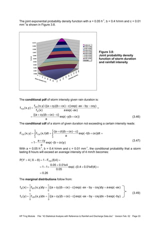
Example 3.6: Bivariate exponential and normal distribution
Assume that storm duration and intensity, (X and Y), are both distributed according to an
exponential distribution (see Kottegoda and Rosso, 1997):
FX(x) = 1 – exp(-ax), x ≥ 0; a > 0 FY(y) = 1 - exp(-by), y ≥ 0; b > 0 (3.43)
Their joint cdf given as a bivariate exponential distribution reads:
(3.44)
Hence, with (3.32), the joint pdf becomes:
(3.45)
)y(F).x(F)yY(P).xX(P)yYxX(PF YXXY =≤≤=≤∩≤=
)y(f).x(f)y,x(f YXXY =
[ ] dxdy)y,x(fyxYXE XY
mkmk'
m,k ∫∫==µ
∞
∞−
∞
∞−
( )( )[ ] ∫ ∫ µ−µ−=−−=
∞
∞−
∞
∞−
dxdy)y,x(f)y)(x(]Y[EY]X[EXEC XYYXXY
0dy)y(f)y(dx)x(f)x(C YYXXXY =∫ µ−∫ µ−=
∞
∞−
∞
∞−
YX
XY
YYXX
XY
XY
C
CC
C
σσ
==ρ
abc0and0b,0a;0y,x:with
)cxybyaxexp()byexp()axexp(1)y,x(FXY
≤≤>>≥
−−−+−−−−=
)cxybyaxexp(}c)cxb)(cya{(
)}cxybyaxexp()cya()axexp(a{
y
x
)y,x(F
yyx
)y,x(F
)y,x(f XYXY
2
XY
−−−−++=
=−−−+−−
∂
∂
=
=
∂
∂
∂
∂
=
∂∂
∂
=](https://image.slidesharecdn.com/download-manuals-hydrometeorology-dataprocessing-43statisticalanalysiswithreftorainfall-140512060654-phpapp01/85/Download-manuals-hydrometeorology-data-processing-43statisticalanalysiswithreftorainfall-42-320.jpg)
![HP Trng Module File: “43 Statistical Analysis with Reference to Rainfall and Discharge Data.doc” Version Feb. 02 Page 35
function G(s), which is the expectation of exp(sX): G(s) = E[exp(sX)]. In case of a
continuous distribution:
(3.50)
Assuming that differentiation under the integral sign is permitted one obtains:
(3.51)
For s = 0 it follows: exp(sx) = 1, and the right hand side of (3.51) is seen to equal the kth
moment about the origin:
(3.52)
Of course this method can only be applied to distributions for which the integral exists.
Similar to the one-dimensional case, the moment generating function for bivariate
distributions is defined by:
(3.53)
of which by partial differentiation to s and t the moments are found.
Example 3.7: Moment generating function for exponential distribution
The moment generating function for an exponential distribution and the k-th moments are
according to (3.50) and (3.52):
(3.54)
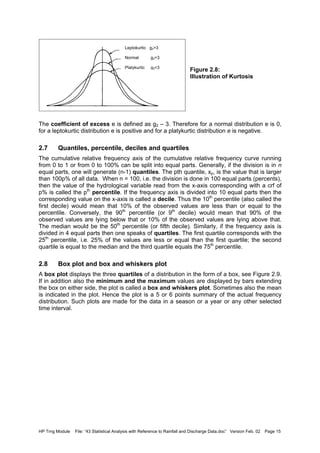
3.2.5 Derived distributions
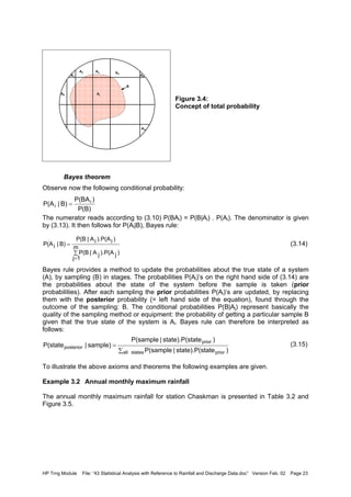
Consider the variables X and Y and their one to one relationship Y = h(X). Let the pdf of X
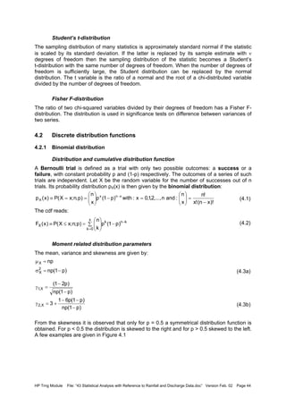
be fX(x), then what is the pdf of Y? For this, consider Figure 3.11. It is observed that the
probability that X falls in the interval x, x + dx equals the probability that Y falls in the interval
y, y + dy. Hence,
fY(y)dy = fX(x)dx (3.55)
[ ] ∫==
∞
∞−
dx)x(f)sxexp()sXexp(E)s(G X
∫=
∞
∞−
dx)x(f)sxexp(x
ds
)s(Gd
X
k
k
k
[ ]
0s
k
k
)k()k(k
ds
Gd
)0(G:where)0(GXE
=
==
[ ] ∫ +∫=+= dxdy)y,x(f)tysxexp((tysxexp(E)t,s(H XY
k
0s
1k
0s
k
k
k
33
0s
4
0s
3
3
3
2
0s
3
0s
2
2
2
0s
2
0s
0
!k
)s(
xk...x3x2
ds
Gd
]X[E
........
63x2
)s(
3x2
ds
Gd
]X[E
2
)s(
2
ds
Gd
]X[E
1
)s(ds
dG
]X[E
s
dx)xexp()sxexp()s(G
λ
=
−λ
λ
==
λ
=
λ
=
−λ
λ
==
λ
=
−λ
λ
==
λ
=
−λ
λ
==
∫
−λ
λ
=λ−λ=
=
+
=
==
==
==
∞](https://image.slidesharecdn.com/download-manuals-hydrometeorology-dataprocessing-43statisticalanalysiswithreftorainfall-140512060654-phpapp01/85/Download-manuals-hydrometeorology-data-processing-43statisticalanalysiswithreftorainfall-45-320.jpg)
![HP Trng Module File: “43 Statistical Analysis with Reference to Rainfall and Discharge Data.doc” Version Feb. 02 Page 36
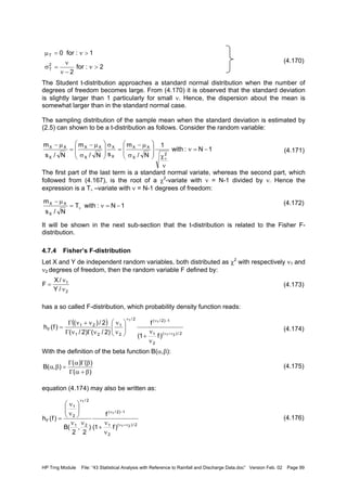
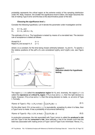
Since fY(y) cannot be negative, it follows:
(3.56)
where the first derivative is called the Jacobian of the transformation, denoted by J.
In a similar manner bivariate distributions can be transformed.
Figure 3.11:
Definition sketch for derived
distributions
Example 3.8: Transformation of normal to lognormal pdf
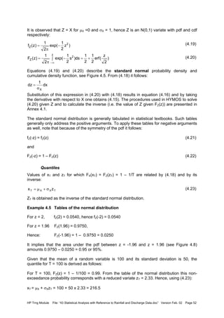
A variable Y is said to have a logarithmic normal or shortly log-normal distribution if its
logarithm is normally distributed, hence ln(Y) = X. So:
3.2.6 Transformation of stochastic variables
Consider the function Z = a + bX + cY, where X, Y and Z are stochastic variables and a, b
and c are coefficients. Then for the mean and the variance of Z it follows:
E[Z] = E[a + bX + cY] = a + bE[X] + cE[Y] (3.57)
E[(Z – E[Z])2
] = E[(a + bX + cY – a – bE[X] – cE[Y])2
] =
= E[b2
(X - E[X])2
+ c2
(Y - E[Y])2
+ 2bc(X - E[X])(Y - E[Y])] =
= b2
E[(X - E[X])2
] + c2
E[(Y - E[Y])2
] + 2bcE[(X - E[X])(Y - E[Y])]
)x(fJ)y(for
dy
dx
)x(f)y(f XYXY ==
Y=h(X)
XfY(y)
YfX(x)
fY(y)
fX(x)
Shaded areas
are equal
Shaded areas
are equal
dy
dx
∞<<
σ
µ−
−
σπ
=
=
=
∞<<∞−
σ
µ−
−
σπ
=
Y0
yln
2
1
exp
y2
1
)y(f
y
1
dy
dx
)Yln(X
X
x
2
1
exp
2
1
)x(f
2
Yln
Yln
)Yln(
Y
2
X
X
X
X](https://image.slidesharecdn.com/download-manuals-hydrometeorology-dataprocessing-43statisticalanalysiswithreftorainfall-140512060654-phpapp01/85/Download-manuals-hydrometeorology-data-processing-43statisticalanalysiswithreftorainfall-46-320.jpg)
![HP Trng Module File: “43 Statistical Analysis with Reference to Rainfall and Discharge Data.doc” Version Feb. 02 Page 37
or:
Var(Z) = b2
Var(X) + c2
Var(Y) + 2bcCov(X,Y) (3.58)
Equations (3.57) and (3.58) are easily extendible for any linear function Z of n-random
variables:
(3.59)
(3.60)
Or in matrix notation by considering the vectors:
(3.61)
(3.62)
The matrix [V] contains the following elements:
(3.63)
This matrix is seen to be symmetric, since Cov(Xi,Xj) = Cov(Xj,Xi). This implies [V] = [V]T
.
Furthermore, since the variance of a random variable is always positive, so is Var([a]T
[X]).
Taylor’s series expansion
For non-linear relationships it is generally difficult to derive the moments of the dependent
variable. In such cases with the aid of Taylor’s series expansion approximate expressions for
the mean and the variance can be obtained. If Z = g(X,Y), then (see e.g. Kottegoda and
Rosso (1997)):
∑∑∑
∑ ∑
∑
= ==
= =
=
==
µ==
=
n
1i
n
1j
jiji
n
1i
ii
n
1i
n
1i
iiii
n
1i
ii
)XX(Covaa)Xa(Var)Z(Var
a]X[Ea]Z[E
XaZ
)])[]])([[](([E][:where
]][[][])[])[]])([[]([]([E])[]([Var)(Var
][])([E:where
][][])([E][])[]([E][E
X
.
.
X
X
X
][
a
.
.
a
a
a
][
T
TTTT
TTT
n
3
2
1
n
3
2
1
µ−µ−=
=µ−µ−==
µ=
µ===
=
=
XXV
aVaaXXaXaZ
X
aXaXaZ
Xa
=
)X(Var.............)X,X(Cov)X,X(Cov
.
.
.
)X,X(Cov..................)X(Var)X,X(Cov
)X,X(Cov...................)X,X(Cov)X(Var
][
n2n1n
n2221
n1211
V](https://image.slidesharecdn.com/download-manuals-hydrometeorology-dataprocessing-43statisticalanalysiswithreftorainfall-140512060654-phpapp01/85/Download-manuals-hydrometeorology-data-processing-43statisticalanalysiswithreftorainfall-47-320.jpg)
![HP Trng Module File: “43 Statistical Analysis with Reference to Rainfall and Discharge Data.doc” Version Feb. 02 Page 38
(3.64)
Above expressions are easily extendable to more variables. Often the variables in g(..) can
be considered to be independent, i.e. Cov(..) = 0. Then (3.64) reduces to:
(3.65)
Example 3.9
Given a function Z = X/Y, where X and Y are independent. Required are the mean and the
variance of Z.
Use is made of equation (3.65). The coefficients read:
(3.66)
Hence:
(3.67)
Example 3.10: Joint cumulative distribution function
The joint pdf of X and Y reads:
Q: determine the probability that 2<X<5 and 1<Y<7
A: the requested probability is obtained from:
)Y,X(Cov
y
g
x
g
2)Y(Var
y
g
)X(Var
x
g
)Z(Var
)Y,X(Cov
yx
g
)Y(Var
y
g
2
1
)X(Var
x
g
2
1
),(g]Z[E
22
2
2
2
2
2
YX
∂
∂
∂
∂
+
∂
∂
+
∂
∂
≈
∂∂
∂
+
∂
∂
+
∂
∂
+µµ≈
)Y(Var
y
g
)X(Var
x
g
)Z(Var
)Y(Var
y
g
2
1
)X(Var
x
g
2
1
),(g]Z[E
22
2
2
2
2
YX
∂
∂
+
∂
∂
≈
∂
∂
+
∂
∂
+µµ≈
32
2
2
2
2
y
x2
y
g
y
x
y
g
0
x
g
y
1
x
g
=
∂
∂
−=
∂
∂
=
∂
∂
=
∂
∂
( )
( )2
vY
2
vX
2
Y
X
2
Y
2
Y
2
X
2
X
2
Y
X2
Y
2
2
Y
X2
X
2
Y
2
vY
Y
X2
Y3
Y
X
Y
X
CC
1
)Z(Var
C1]Z[E
+
µ
µ
=
µ
σ
+
µ
σ
µ
µ
=σ
µ
µ
+σ
µ
≈
+
µ
µ
=σ
µ
µ
+
µ
µ
≈
0y,0x:for0)y,x(f
0y,0x:for)2/yxexp()y,x(f
XY
XY
≤≤=
>>−−=
0741.0))6065.0(0302.0))(1353.0(0067.0(
))2/yexp(2)()xexp((dy)2/yexp(dx)xexp(dxdy)y,x(f)7Y15X2(P
7
1
5
2
7
1
5
2
7
1
5
2XY
=−−−−−−=
=−−−−=−−==<<∩<< ∫∫ ∫ ∫](https://image.slidesharecdn.com/download-manuals-hydrometeorology-dataprocessing-43statisticalanalysiswithreftorainfall-140512060654-phpapp01/85/Download-manuals-hydrometeorology-data-processing-43statisticalanalysiswithreftorainfall-48-320.jpg)
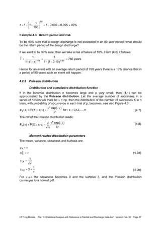

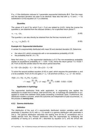
![HP Trng Module File: “43 Statistical Analysis with Reference to Rainfall and Discharge Data.doc” Version Feb. 02 Page 50
The uniform distribution is of particular importance for data generation, where with a = 0 and
b = 1 the density function provides a means to generate the non-exceedance probabilities. It
provides also a means to assess the error in measurements due to limitations in the scale. If
the scale interval is c, it implies that an indicated value is ± ½ c and the standard deviation of
the measurement error is σ = √(c2
/12) ≈ 0.3c.
4.4 Normal distribution related distributions
4.4.1 Normal Distribution
Four conditions are necessary for a random variable to have a normal or Gaussian
distribution (Yevjevich, 1972):
• A very large number of causative factors affect the outcome
• Each factor taken separately has a relatively small influence on the outcome
• The effect of each factor is independent of the effect of all other factors
• The effect of various factors on the outcome is additive.
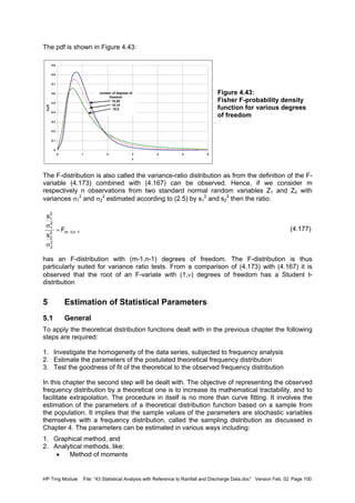
Probability density and cumulative frequency distribution
The pdf and cdf of the normal distribution read:
(4.15)
(4.16)
where: x = normal random variable
µX, σX = parameters of the distribution, respectively the mean and the
standard deviation of X.
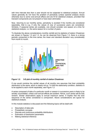
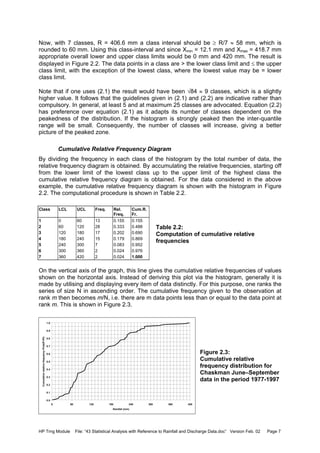
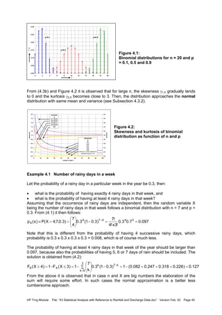
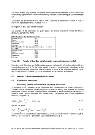
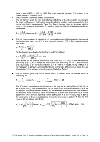
The pdf and cdf are displayed in Figure 4.5.
Figure 4.5:
Normal probability density and
cumulative density functions for µ = 0
and σ = 1
The normal pdf is seen to be a bell-shaped symmetric distribution, fully defined by the two
parameters µX and σX. The coefficient (σX√(2π))-1
in Equation (4.15) is introduced to ensure
that the area under the pdf-curve equals unity, because the integral:
0and,xwith
x
2
1
exp
2
1
(x)f XX
2
X
X
X
X >σ∞<µ<∞−∞<<∞−
σ
µ−
−
πσ
=
ds
s
2
1
exp
2
1
]xX[P)x(F
2
X
X
x
X
X
σ
µ−
−∫
πσ
=≤≡
∞−
0.00
0.05
0.10
0.15
0.20
0.25
0.30
0.35
0.40
0.45
0.50
-3 -2 -1 0 1 2 3
x
pdff(x)
0
0.1
0.2
0.3
0.4
0.5
0.6
0.7
0.8
0.9
1
cdfF(x)
normal
probability
normal cumulative
density function
a
dx)axexp(2dx)axexp(
0
22 π
=∫ −∫ =−
∞∞
∞−](https://image.slidesharecdn.com/download-manuals-hydrometeorology-dataprocessing-43statisticalanalysiswithreftorainfall-140512060654-phpapp01/85/Download-manuals-hydrometeorology-data-processing-43statisticalanalysiswithreftorainfall-60-320.jpg)
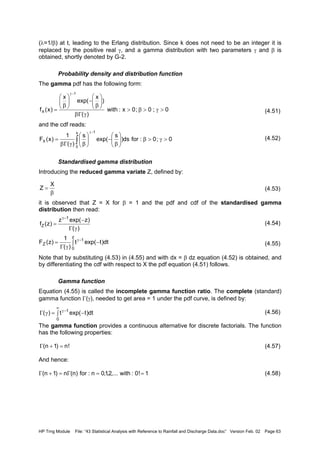
![HP Trng Module File: “43 Statistical Analysis with Reference to Rainfall and Discharge Data.doc” Version Feb. 02 Page 53
Figure 4.8:
Use of symmetry of standard normal
pdf around 0 to find non-exceedance
probabilities
Some Properties of the Normal Distribution
1. A linear transformation Y = a + bX of an N(µX, σX
2
) random variable X makes Y an N(a +
bµX, b2
σX
2
) random variable.
2. If Sn is the sum of n independent and identically distributed random variables Xi each
having a mean µX and variance σX
2
, then in the limit as n approaches infinity, the
distribution of Sn approaches a normal distribution with mean nµX and variance nσX
2
.
3. Combining 1 and 2, for the mean Xm of Xi it follows, using the statement under 1 with a =
0 and b = 1/n, that Xm tends to have an N(µX, σX
2
/n) distribution as n approaches infinity:
If Xi is from an N(µX, σX
2
) population, then the result for the sum and the mean holds
regardless of the sample size n. The Central Limit Theorem, though, states that
irrespective of the distribution of Xi the sum Sn and the mean Xm will tend to normality
asymptotically. According to Haan (1979) if interest is in the main bulk of the distribution of
Sn or Xm then n as small as 5 or 6 will suffice for approximate normality, whereas larger n is
required for the tails of the distribution of Sn or Xm. It can also be shown that even if the Xi’s
have different means and variances the distribution of Sn will tend to be normal for large n
with N(ΣµXi; ΣσXi
2
), provided that each Xi has a negligible effect on the distribution of Sn, i.e.
there are no few dominating Xi’s.
An important outcome of the Central Limit Theorem is that if a hydrological variable is the
outcome of n independent effects and n is relatively large, the distribution of the variable is
approximately normal.
Application in hydrology
The normal distribution function is generally appropriate to fit annual rainfall and annual
runoff series, whereas quite often also monthly rainfall series can be modelled by the normal
distribution. The distribution also plays an important role in modelling random errors in
measurements.
0.00
0.05
0.10
0.15
0.20
0.25
0.30
0.35
0.40
0.45
0.50
-3 -2 -1 0 1 2 3
x
pdff(x)
0
0.1
0.2
0.3
0.4
0.5
0.6
0.7
0.8
0.9
1
cdfF(x)
0.95
[ ] [ ] [ ]
( ) ( ) ( ) ( ) ( ) ( )
n
xVarn
n
1
xVar
n
1
xVar
n
1
xVar
n
1
xVar
n
1
mVar
n.
n
1
xE
n
1
EE
n
1
mE:sox
n
1
x
n
1
x
n
1
x
n
1
m
2
x
2i2n2i2i2x
xxixxn21
1i
ix i
σ
=⋅==+++=
µ=µ===+++==
∑
∑∑
=
L
L](https://image.slidesharecdn.com/download-manuals-hydrometeorology-dataprocessing-43statisticalanalysiswithreftorainfall-140512060654-phpapp01/85/Download-manuals-hydrometeorology-data-processing-43statisticalanalysiswithreftorainfall-63-320.jpg)
![HP Trng Module File: “43 Statistical Analysis with Reference to Rainfall and Discharge Data.doc” Version Feb. 02 Page 57
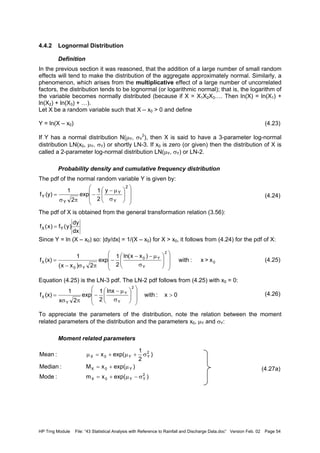
For LN-3 the inverse relations are more complex as the starting point is the cubic equation in
η relating η and γ1,X, from (4.27b):
(4.30)
The parameters of the LN-3 distribution can be expressed in η (i.e. γ1,X), µX and σX :
(4.31)
The parameters of the LN-3 distribution can be expressed in η (i.e. γ1,X), µX and σX:
(4.32)
(4.33)
(4.34)
If the parameters would be determined according to equations (4.32) to (4.34) one observes
that the shape parameter σY is solely determined by the skewness, the scale parameter µY
by the variance and the skewness and the location parameter x0 by the first three moments.
Moment generating function
The expressions presented in (4.27a/b) can be derived by observing that:
Hence, the power of the exponential can be replaced by:
The last integral is seen to be 1, hence it follows for E[(X-x0)k
] = E[exp(kY)]:
(4.35)
03 X,1
3
=γ−η+η
3/1
2
X,1X,1
3/1
2
X,1X,1
2
1
22
1
2
γ
++
γ
−−
γ
++
γ
=η
η
σ
−µ= X
X0x
)1ln( 2
Y +η=σ
+ηη
σ
=σ−−µ=µ
)1(
ln
2
1
2
1
)xln( 22
2
X2
Y0XY
( )
:followsitk
y
u:with
dy
y
2
1
kyexp
2
1
)]kY[exp(Edy
y
2
1
exp(
2
1
)kyexp(dx)x(f)xx(])xX[(E
Y
Y
Y
y
2
y
2
Y
Y
Y
X
k
0
k
0
σ−
σ
µ−
=
σ
µ−
−
πσ
=
==
σ
µ−
−
πσ
=−=−
∫
∫ ∫
∞
∞−
∞
∞−
∞
∞−
)k
2
1
kexp(])xX[(E 2
Y
2
Y
k
0 σ+µ=−
( ) 2
y
2
y
2
y
y
2
y
y
y2
kyk2
y
k
y
u σ+µ−−
σ
µ−
=
σ−
σ
µ−
=
22
y
2
y
2
y
y2
y
2
y
2
y
y2
u
2
1
k
2
1
k
y
2
1
ky:ork
2
1
kky
y
2
1
u
2
1
−σ+µ=
σ
µ−
−σ−µ−+
σ
µ−
−=−
:getsonedudy:ordy
1
du:withandu
2
1
k
2
1
k y
y
22
y
2
y σ=
σ
=−σ+µ
du)u
2
1
exp(
2
1
)k
2
1
kexp()]kY[exp(E 22
Y
2
Y −
π
σ+µ= ∫
∞
∞−](https://image.slidesharecdn.com/download-manuals-hydrometeorology-dataprocessing-43statisticalanalysiswithreftorainfall-140512060654-phpapp01/85/Download-manuals-hydrometeorology-data-processing-43statisticalanalysiswithreftorainfall-67-320.jpg)
![HP Trng Module File: “43 Statistical Analysis with Reference to Rainfall and Discharge Data.doc” Version Feb. 02 Page 68
(4.72)
(4.73)
From the last expression it is observed that:
(4.74)
The term within brackets can be seen as an adjusted coefficient of variation, and then the
similarity with Equation (4.63) is observed.
Moment generating function
The moments of the distribution are easily obtained from the moment generating function:
(4.75)
Or introducing the reduced variate Z = (x-x0)/β, and dx = β dz:
Introducing further: u = z(1-sβ), or z = u/(1-sβ) and dz = 1/(1-sβ)du, it follows:
(4.76)
By taking the derivatives of G(s) with respect to s at s = 0 the moments about the origin can
be obtained:
Since for the computation of the central moments the location parameter is of no importance,
the moment generating function can be simplified with x0 = 0 to:
(4.78)
Using equation (3.30) the central moments can be derived from the above moments about
the origin.
X,1
X
X0 2x
γ
σ
−µ=
−µ
σ
=γ
0X
X
X,1
x
2
dx
)(
xx
exp
xx
)sxexp()]sx[exp((E)s(G
0x
0
1
0
∫
∞
−γ
γΓβ
β
−
−
β
−
==
dz
)(
)s1(zexp(z
)sxexp()s(G
0
1
0 ∫
γΓ
β−−
=
∞ −γ
γ−
∞ −γ
γ−
β−=
=
γΓ
−
β−= ∫
)s1)(sxexp(
du
)(
)uexp(u
)s1)(sxexp()s(G
0
0
1
0
βγ+=µ=µ
β−βγ+β−=µ=
=
+γ−γ−
0X
'
1
0s
)1(
00
'
1
x:so
})s1()s1(x){sxexp(
ds
)0(dG
.etc
)1()s1)(1(
ds
)0(Gd
)s1(
ds
)0(dG
:hence
)s1()s(G
2'
2
0s
)2(2
2
2
0x
'
1
0s
)1(
0
+γγβ=µ→β−+γγβ=
βγ=µ→β−βγ=
β−=
=
+γ−
==
+γ−
λ−](https://image.slidesharecdn.com/download-manuals-hydrometeorology-dataprocessing-43statisticalanalysiswithreftorainfall-140512060654-phpapp01/85/Download-manuals-hydrometeorology-data-processing-43statisticalanalysiswithreftorainfall-78-320.jpg)
![HP Trng Module File: “43 Statistical Analysis with Reference to Rainfall and Discharge Data.doc” Version Feb. 02 Page 85
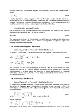
4.6.5 Extreme value Type 3 distribution
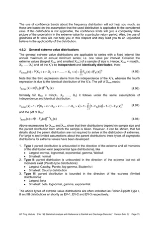
EV-3 for largest value
The Extreme Value Type III distribution for largest value is given by (4.101) and is defined
for x ≤ x0, k > 0 and β > 0
(4.101)
The pdf reads:
(4.135)
The mean, median, mode, variance and skewness are given by:
(4.136a)
(4.136b)
Note that these expressions are similar to those of the smallest value modelled as EV-2.
Above moment related parameters are easily obtained from the rth
moment of (x0 – Xmax)
which can shown to be:
(4.137)
To simplify the computation, note that for the higher moments x0 can be omitted, so for r > 1
one can put x0 = 0 and use (3.30). Equation (4.137) then simplifies to:
So:
The fact that Xmax is bounded by x0 makes that EV-3 is seldom used in hydrology for
modelling the distribution of Xmax. Its application only make sense, if there is a physical
reason that limits Xmax to x0.
EV-3 for smallest value
The extreme value Type III distribution for the smallest value, for x ≥ x0, k > 0 and β > 0, has
the following form:
(4.106)
)rk1()1( rr'
r +Γβ−=µ
)k31(
)k21(
3'
3
2'
2
+Γβ−=µ
+Γβ=µ
β
−
−−=
k/1
0
maxX
xx
exp)x(F
β
−
−−
β
−
−
β
=
− k/1
0
1k/1
0
maxX
xx
exp
xx
k
1
)x(f
k
0maxX
k
0maxX
0maxX
)k1(xm
)2(lnxM
)k1(x
−β−=
β−=
+Γβ−=µ
{ }
( ) 2/32
3
maxX,1
222
maxX
)k1()k21(
)k1(2)k21()k1(3)k31(
)k1()k21(
+Γ−+Γ
+Γ++Γ+Γ−+Γ
−=γ
+Γ−+Γβ=σ
[ ] )rk1()Xx(E rr
max0 +Γβ=−
)
xx
exp(1)x(F
k/1
0
minX
β
−
−−=](https://image.slidesharecdn.com/download-manuals-hydrometeorology-dataprocessing-43statisticalanalysiswithreftorainfall-140512060654-phpapp01/85/Download-manuals-hydrometeorology-data-processing-43statisticalanalysiswithreftorainfall-95-320.jpg)
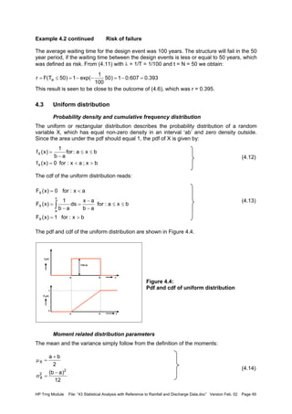
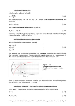
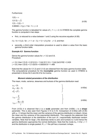
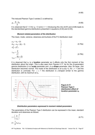
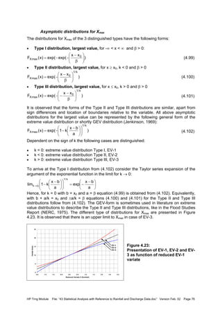
![HP Trng Module File: “43 Statistical Analysis with Reference to Rainfall and Discharge Data.doc” Version Feb. 02 Page 89
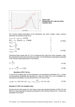
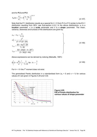
Figure 4.30:
Cdf of Pareto distribution for
various of shape parameter
Quantiles
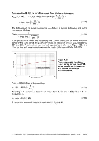
The quantiles, referring to a return period of T years, follow from (4.143) to (1.145) and read:
• For Type I distribution P-1:
(4.150)
• For Type II and III distributions, P-2, P-3:
(4.151)
Note that above two expressions should not directly be applied to exceedance series unless
the number of data points coincide with the number of years, see next sub-section.
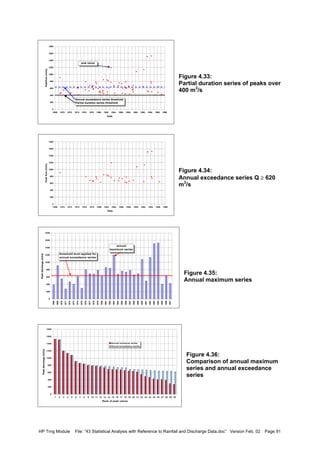
4.6.7 Relation between maximum and exceedance series
The GEV distributions are applicable to series with a fixed interval, e.g. a year: series of the
largest or smallest value of a variable each year, like annual maximum or minimum flows. If
one considers largest values, such a series is called an annual maximum series. Similarly,
annual minimum series can be defined.
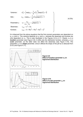
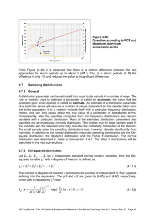
In contrast to this, one can also consider series of extreme values above or below a certain
threshold value, i.e. the maximum value between an upcrossing and a downcrossing or the
minimum between a downcrossing and an upcrossing, see Figure 4.31.
Figure 4.31:
Definition of partial duration or
peaks over threshold series
Tlnxx 0T σ+=
)T1(xx 0T
θ−
−
θ
σ
+=
T im e in d ays
27-03-199512-03-199525-02-199510-02-199526-01-199511-01-199527-12-199412-12-1994
Discharge[m3/s]
1,600
1,500
1,400
1,300
1,200
1,100
1,000
900
800
700
600
500
400
300
200
100
0
upcrossing downcrossing
threshold
Peaks over threshold
0.0
0.1
0.2
0.3
0.4
0.5
0.6
0.7
0.8
0.9
1.0
0.0 0.5 1.0 1.5 2.0 2.5 3.0 3.5 4.0 4.5 5.0
Z
FZ(z)
θ-parameter
0.75
0.50
0.25
0.00
-0.25
-0.50](https://image.slidesharecdn.com/download-manuals-hydrometeorology-dataprocessing-43statisticalanalysiswithreftorainfall-140512060654-phpapp01/85/Download-manuals-hydrometeorology-data-processing-43statisticalanalysiswithreftorainfall-99-320.jpg)
![HP Trng Module File: “43 Statistical Analysis with Reference to Rainfall and Discharge Data.doc” Version Feb. 02 Page 90
The series resulting from exceedance of a base or threshold value x0 thereby considering
only the maximum between an upcrossing and a downcrossing is called a partial duration
series (PDS) or peaks over threshold series, POT-series. The statistics may be developed
for the exceedance of the value relative to the base only or for the value as from zero. The
latter approach will be followed here. In a similar manner partial duration series for non-
exceedance of a threshold value can be defined. When considering largest values, if the
threshold is chosen such that the number of exceedances N of the threshold value equals
the number of years n, the series is called annual exceedance series. So, if there are n
years of data, in the annual exceedance series the n largest independent peaks out of N ≥ n
are considered. To arrive at independent peaks, there should be sufficient time between
successive peaks. The physics of the process determines what is a sufficient time interval
between peaks to be independent; for flood peaks a hydrograph analysis should be carried
out. The generalised Pareto distribution is particularly suited to model the exceedance
series.
Note that there is a distinct difference between annual maximum and annual exceedance
series. In an annual maximum series, for each year the maximum value is taken, no matter
how low the value is compared to the rest of the series. Therefore, the maximum in a
particular year may be less than the second or the third largest in another year, which values
are considered in the annual exceedance series if the ranking so permits. Hence the lowest
ranked annual maximums are less than (or at the most equal to) the tail values of the ranked
annual exceedance series values.
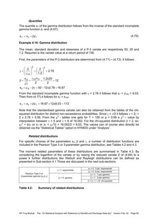
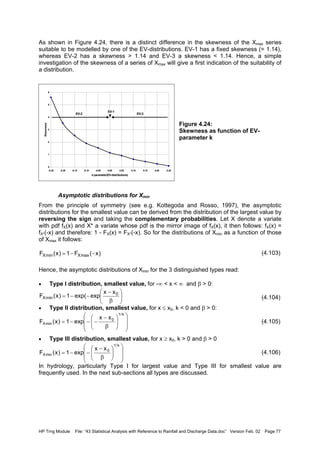
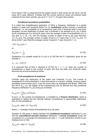
The procedure to arrive at the annual exceedance series via a partial duration series and its
comparison with the annual maximum series is shown in the following figures, from a record
of station Chooz on Meuse river in northern France (data 1968-1997). The original discharge
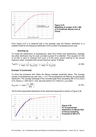
series is shown in Figure 4.32. Next a threshold level of 400 m3
/s has been assumed. The
maximum values between each upcrossing and the next downcrossing are considered. In
this particular case, peaks which are distanced ≥ 14 days apart are expected to be
independent and are included in the partial duration series, shown in Figure 4.33. This
results in 72 peaks. Since there are 30 years of record, the partial duration series has to be
reduced to the 30 largest values. For this the series values are ranked in descending order
and the first 30 values are taken to form the annual exceedance series. The threshold value
for the annual exceedance series appears to 620 m3
/s. The annual exceedance series is
shown in Figure 4.34. It is observed that some years do not contribute to the series, as their
peak values were less than 620 m3
/s, whereas other years contribute with 2 or some even
with 3 peaks. The annual maximum series is presented in Figure 4.35, together with the
threshold for the annual exceedance series. It is observed that indeed for a number of years
that threshold level was not reached. A comparison of the two series is depicted in Figure
4.36.
Figure 4.32:
Discharge series of station chooz
on Meuse river with applied
threshold Q = 400 m3
/s
28-10-199528-12-199127-02-198828-04-198428-06-198028-08-197628-10-197228-12-1968
Discharge[m3/s]
1,600
1,500
1,400
1,300
1,200
1,100
1,000
900
800
700
600
500
400
300
200
100
0
Applied
threshold](https://image.slidesharecdn.com/download-manuals-hydrometeorology-dataprocessing-43statisticalanalysiswithreftorainfall-140512060654-phpapp01/85/Download-manuals-hydrometeorology-data-processing-43statisticalanalysiswithreftorainfall-100-320.jpg)
![HP Trng Module File: “43 Statistical Analysis with Reference to Rainfall and Discharge Data.doc” Version Feb. 02 Page 101
• Maximum likelihood method
• Method of least squares
• Mixed moment-maximum likelihood method, etc.
Estimation error
The parameters estimated with the above methods differ. To compare the quality of different
estimators of a parameter, some measure of accuracy is required. The following measures
are in use:
• mean square error and root mean square error
• error variance and standard error
• bias
• efficiency
• consistency
Mean square error
A measure for the quality of an estimator is the mean square error, mse. It is defined by:
(5.1)
where φ is an estimator for Φ.
Hence, the mse is the average of the squared differences between the sample value and the
true value. Equation (5.1) can be expanded to the following expression:
(5.2)
Since:
(5.3)
and:
(5.4)
it follows that:
(5.5)
The mean square error is seen to be the sum of two parts:
• the first term is the variance of φ, equation (5.3), i.e. the average of the squared
differences between the sample value and the expected mean value of φ based on the
sample values, which represents the random portion of the error, and
• the second term of (5.5) is the square of the bias of φ, equation (5.4), describing the
systematic deviation of expected mean value of φ from its true value Φ, i.e. the
systematic portion of the error.
Note that if the bias in φ is zero, then mse = σφ
2
. Hence, for unbiased estimators, i.e. if
systematic errors are absent, the mean square error and the variance are equivalent. If
mse(φ1) < mse (φ2) then φ1 is said to be more efficient than φ2 with respect to Φ.
])[(Emse 2
Φ−φ=
])][E[(E]])[E[(Emse 22
Φ−φ+φ−φ=
[ ]( )[ ] 22
EE φσ=φ−φ
22
b])][E[(E φ=Φ−φ
22
bmse φφ +σ=](https://image.slidesharecdn.com/download-manuals-hydrometeorology-dataprocessing-43statisticalanalysiswithreftorainfall-140512060654-phpapp01/85/Download-manuals-hydrometeorology-data-processing-43statisticalanalysiswithreftorainfall-111-320.jpg)
![HP Trng Module File: “43 Statistical Analysis with Reference to Rainfall and Discharge Data.doc” Version Feb. 02 Page 102
Root mean square error
Instead of using the mse it is customary to work with its square root to arrive at an error
measure, which is expressed in the same units as Φ, leading to the root mean square
(rms) error:
(5.6)
Standard error
When discussing the frequency distribution of statistics like of the mean or the standard
deviation, for the standard deviation σφ the term standard error is used, e.g. standard error
of the mean and standard error of the standard deviation, etc.
(5.7)
In Table 5.1, a summary of unbiased estimators for moment parameters is given, together
with their standard error. With respect to the latter it is assumed that the sample elements
are serially uncorrelated. If the sample elements are serially correlated a so-called
effective number of data Neff has to be applied in the expressions for the standard error in
Table 5.1
Consistency
If the probability that φ approaches Φ becomes unity if the sample becomes large then the
estimator is said to be consistent or asymptotically unbiased:
(5.8)
To meet this requirement it is sufficient to have a zero mean square error in the limit for
n→∞.
5.2 Graphical estimation
In graphical estimations, the variate under consideration is regarded as a function of the
standardised or reduced variate with known distribution. With a properly chosen probability
scale a linear relationship can be obtained between the variate and the reduced variate
representing the transformed probability of non-exceedance. Consider for this the Gumbel
distribution. From (4.108) it follows:
(5.9)
According to the Gumbel distribution the reduced variate z is related to the non-exceedance
probability by:
(5.10)
To arrive at an estimate for x0 and β we plot the ranked observations xi against zi by
estimating the non-exceedance probability of xi, i.e. Fi. The latter is called the plotting
position of xi, i.e. the probability to be assigned to each data point to be plotted on probability
paper. Basically, appropriate plotting positions depend on the distribution function one
wants to fit the observed distribution function to. A number of plotting positions has been
proposed, which is summarised in Table 5.4.To arrive at an unbiased plotting position for the
Gumbel distribution Gringorten’s plotting position has to be applied, which reads:
222
b])[(Ermse φφ +σ=Φ−φ=
]])[E[(E 2
φ−φ=σφ
ε=ε>Φ−ϕ∞→ anyfor0)||(obPrlimn
zxx 0 β+=
))x(Fln(ln(z X−−=](https://image.slidesharecdn.com/download-manuals-hydrometeorology-dataprocessing-43statisticalanalysiswithreftorainfall-140512060654-phpapp01/85/Download-manuals-hydrometeorology-data-processing-43statisticalanalysiswithreftorainfall-112-320.jpg)

![HP Trng Module File: “43 Statistical Analysis with Reference to Rainfall and Discharge Data.doc” Version Feb. 02 Page 107
generally represented by the mean, variance, skewness and kurtosis, are at maximum
required to specify the distribution and to derive the distribution parameters. Most
distributions, however, need only one, two or three parameters to be estimated. It is to be
understood that the higher the order of the moment the larger the standard error will be.
In HYMOS the unbiased estimators for the mean, variance, skewness and kurtosis as
presented by equations (2.3), (2.5) or (2.6), (2.8) and (2.9) are used, see also Table 5.1.
Substitution of the required moments in the relations between the distribution parameters
and the moments will provide the moment estimators:
• Normal distribution: the two parameters are the mean and the standard deviation, which
follow from (2.3) and (2.6) immediately
• LN-2: equations (2.3) and (2.6) substituted in (4.28) and (4.29)
• LN-3: equations (2.3), (2.6) and (2.8) substituted in (4.31) to (4.34)
• G-2: equations (2.3) and (2.6) substituted in (4.61) and (4.62)
• P-3: equations (2.3), (2.6) and (2.8) substituted in (4.71) to (4.73)
• EV-1:equations (2.3) and (2.6) substituted in (4.115) and (4.116)
For all other distributions the method of moments is not applied in HYMOS.
Biased-unbiased
From (2.5) it is observed that the variance is estimated from:
(2.5)
The denominator (N-1) is introduced to obtain an unbiased estimator. A straightforward
estimator for the variance would have been:
(5.13)
The expected value of this estimator, in case the xi’s are independent, is:
(5.14)
From equation (5.14) it is observed that although the estimator is consistent, it is biased.
Hence, to get an unbiased estimator for σX
2
the moment estimator should be multiplied by
N/(N-1), which leads to (2.5)
Remark
The method of moments provides a simple procedure to estimate distribution parameters.
For small sample sizes, say N < 30, the sample moments may differ substantially from the
population values. Particularly if third order moments are being used to estimate the
parameters, the quality of the parameters will be poor if the sample size is small. In such
cases single outliers will have a strong effect on the parameter estimates.
Probability weighted moments and L-moments
The above method of moments is called Product Moments. The negative effects the use of
higher moments have on the parameter estimation is eliminated by making use of L-
moments, which are linear functions of probability weighted moments (PWM’s).
Probability weighted moments are generally defined by:
∑
=
−
−
=
N
1i
2
Xi
2
X )mx(
1N
1
s
∑
=
−=
N
1i
2
Xi
2
X )mx(
N
1
s
)
( ) 2
X
2
X2
X
N
1i
2
XXXi
2
Xi
2
X
N
1N
N
])m()x([E])mx[(E
N
1
]sˆ[E σ
−
=
σ
−σ=µ−−µ−=−= ∑
=
{ } { }[ ]s
X
r
X
p
s,r,p )x(F1)x(FXEM −=](https://image.slidesharecdn.com/download-manuals-hydrometeorology-dataprocessing-43statisticalanalysiswithreftorainfall-140512060654-phpapp01/85/Download-manuals-hydrometeorology-data-processing-43statisticalanalysiswithreftorainfall-117-320.jpg)
![HP Trng Module File: “43 Statistical Analysis with Reference to Rainfall and Discharge Data.doc” Version Feb. 02 Page 108
(5.15)
By choosing p=1 and s=0 in (5.15) one obtains the rth
PWM, which reads:
(5.16)
Comparing this expression with the definition of moments in (3.23) it is observed that instead
of raising the variable to a power ≥ 1 now the cdf is raised to a power ≥ 1. Since the latter
has values < 1, it is observed that these moments are much less sensitive for outliers, which
in the case of product moments strongly affect the moments and hence the parameters to be
estimated.
L-moments are developed for order statistics. Let the XI’s be independent random variables
out of a series of sample of size N, which are put in ascending order:
X1:N < X2:N <….<XN:N
then Xi:N is the ith
largest in a random sample of N, and is known as the ith
order statistic. L-
moments are used to characterize the distribution of order statistics. In practice the first four
L-moments are of importance:
(5.17)
The first moment is seen to be the mean, the second a measure of the spread or scale of the
distribution, the third a measure of asymmetry and the fourth a measure of peakedness.
Dimensionless analogues to the skewness and kurtosis are (Metcalfe, 1997):
(5.18)
The relation between the L-moments and parameters of a large number of distributions are
presented in a number of statistical textbooks. For some distributions they are given below
(taken from Dingman, 2002):
• Uniform distribution
(5.19)
• Normal distribution
{ }[ ] { }∫
∞
∞−
==β dx)x(f)x(Fx)x(FXE X
r
X
r
Xr
[ ]
[ ] [ ]{ }
[ ] [ ] [ ]{ }
[ ] [ ] [ ] [ ]{ }4:14:24:34:44
3:13:23:33
2:12:22
1
XEXE3XE3XE
4
1
XEXE2XE
3
1
XEXE
2
1
XE
−+−=λ
+−=λ
−=λ
=λ
1)15(
4
1
:with:kurtosisL
11:with:skewnessL
4
2
3
2
4
4
3
2
3
3
<τ≤−τ
λ
λ
=τ−
<τ<−
λ
λ
=τ−
0
0
6
ab
2
ba
4
3
2
1
=τ
=τ
−
=λ
+
=λ
1226.0
0
4
3
X
2
X1
=τ
=τ
π
σ
=λ
µ=λ](https://image.slidesharecdn.com/download-manuals-hydrometeorology-dataprocessing-43statisticalanalysiswithreftorainfall-140512060654-phpapp01/85/Download-manuals-hydrometeorology-data-processing-43statisticalanalysiswithreftorainfall-118-320.jpg)
![HP Trng Module File: “43 Statistical Analysis with Reference to Rainfall and Discharge Data.doc” Version Feb. 02 Page 114
The procedure will be shown for LN-3. For given location parameters the MLM estimators for
µY and σY
2
become similar to (5.30) and (5.31) with x replaced by x-x0 respectively:
(5.32)
(5.33)
Next, the first moment relation for the lognormal distribution is taken, (4.27a), to arrive at a
value for x0:
(5.34)
The location parameter x0 is solved iteratively from a modified form of (5.34) as follows:
(5.35)
For each value of x0 the parameters µY and σY
2
are estimated by (5.32) and (5.33). Given an
initial estimate of x0, an improved estimate is obtained by means of the Newton-Raphson
method:
(5.36)
Since µY and σY
2
are also a function of x0 it follows for the derivative g’(x0,old):
(5.37)
To speed up the computations, in HYMOS the expected value of g’(x0,old) is calculated rather
than computing g’(x0,old) for each x0:
(5.38)
By substitution of (5.37) in (5.36) it follows for the improved estimate of x0:
(5.39)
The iteration is continued till:
(5.40)
The initial value of x0 is taken as:
(5.41)
∑
=
−=µ
N
1i
0iY )xxln(
N
1
ˆ
( )∑
=
µ−−=σ
N
1i
2
Y0i
2
Y ˆ)xxln(
N
1
ˆ
σ
+µ−µ=
2
ˆ
ˆexpˆx
2
Y
YX0
0)xˆln(
2
ˆ
ˆ)x(g 0X
2
Y
Y0 =−µ−
σ
+µ=
)x('g
)x(g
xx
old,0
old,0
old,0new,0 −=
1
0
N
1i
X
1
0iY
0
0 )xˆ()xx(
N
1
)1ˆ(
dx
dg
)x('g −
=
−
−µ+−−µ== ∑
0X
2
Y
2
Y
0
xˆ
1)ˆexp()1ˆ(
)]x('g[E
−µ
+σ−σ
=
)ˆexp().1ˆ(1
)xˆ.()xˆln(
2
ˆ
ˆ
xx 2
Y
2
Y
0X0X
2
Y
Y
old,0new,0
σ−σ+
−µ
−µ−
σ
+µ
−=
1000
x
:withxx minX
old,0new,0
−µ
=εε<−
)x(1.0xx minXmin0 −µ−=](https://image.slidesharecdn.com/download-manuals-hydrometeorology-dataprocessing-43statisticalanalysiswithreftorainfall-140512060654-phpapp01/85/Download-manuals-hydrometeorology-data-processing-43statisticalanalysiswithreftorainfall-124-320.jpg)
 = 1.134
Prob(nds.le. nds,obs = .872
Hypothesis: H0: Series is random
H1: Series is not random
A two-tailed test is performed
Level of significance is α 5.00 percent
Critical value for test statistic z1-α/2 = 1.960
Result: H0 not rejected
Test for Significance of Linear Trend
Intercept parameter (=b1) = 871.612
Slope parameter (=b2) = .5401E+00
St.dev. of b2 (=sb2) = .1424E+02
St.dev. of residual (=se) = .3673E+03
Test statistic [Tt] (abs.value) = .038
Degrees of freedom = 18
Prob(Tt.le Tt,obs = .515
Hypothesis: H0: Series is random
2nm
s)1n(s)1m(
n
1
m
1
s
2
Z
2
Y
YZ
−+
−+−
+=
n
s
m
s
m
s
:and
1n
)1(
1m
:and
n
s
m
s
s 2
Z
2
Y
2
Y1
222
Z
2
Y
YZ
+
=ψ
−
ψ−
+
−
ψ
=ν+=
−](https://image.slidesharecdn.com/download-manuals-hydrometeorology-dataprocessing-43statisticalanalysiswithreftorainfall-140512060654-phpapp01/85/Download-manuals-hydrometeorology-data-processing-43statisticalanalysiswithreftorainfall-138-320.jpg)
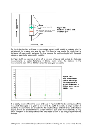
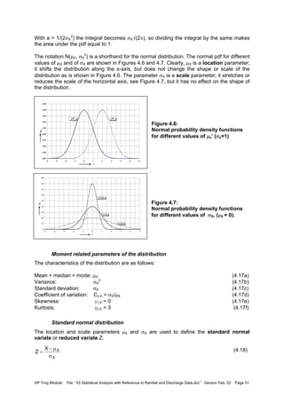
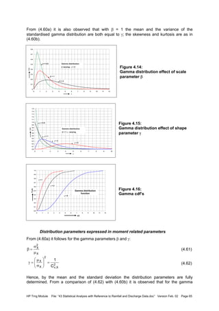
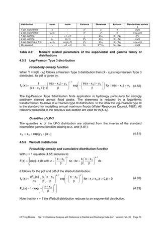
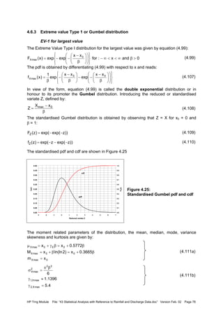
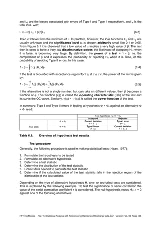
![HP Trng Module File: “43 Statistical Analysis with Reference to Rainfall and Discharge Data.doc” Version Feb. 02 Page 129
H1: Series is not random
A two-tailed test is performed
Level of significance α is 5.00 percent
Critical value for test statistic t ,1-α/2 = 2.101
Result: H0 not rejected
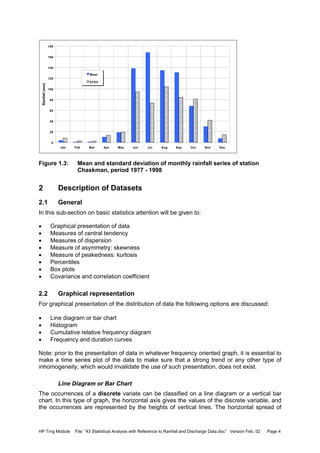
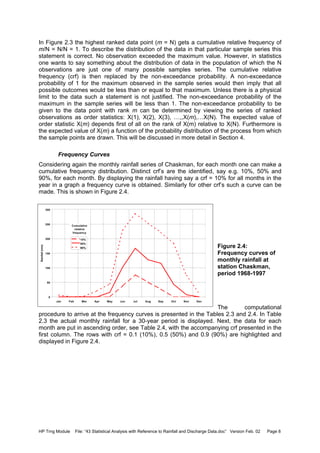
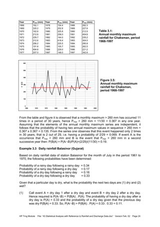
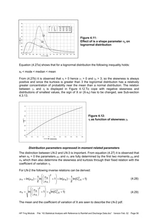
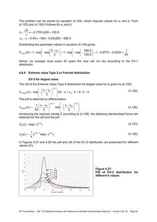
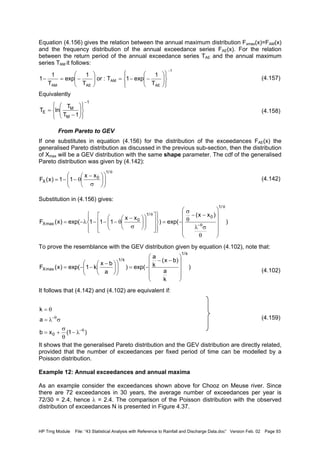
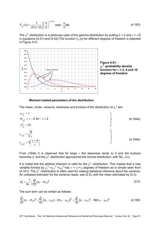
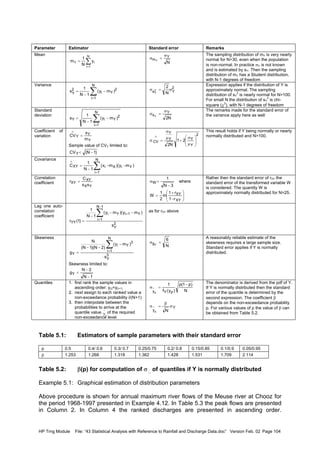
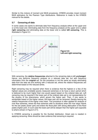
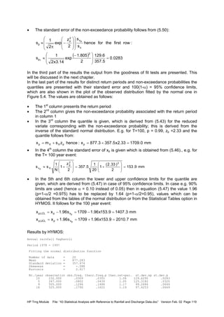
Figure 6.3:
Annual rainfall at Vagharoli,
period 1978-1997, with
division for split sample test
Student t-Test with Welch modification
Number of data in first set = 10
Number of data in second set = 10
Test statistic [TS] (abs.value) = .842
Degrees of freedom = 18
Prob(t.<.[TS]) = .795
Mean of first set (mY) = 809.458
St.dev. of first set (sY) = 397.501
Mean of second set (mZ) = 945.108
St.dev. of second set (sZ) = 318.659
Var. test stat. FS = sY
2
/sZ
2
) = 1.556
Prob(F ≤ FS ) = .740
Hypothesis: H0: Series is homogeneous
H1: Series is not homogeneous
A two-tailed test is performed
Level of significance is α = 5.00 percent
Critical value for test statistic mean t ,1-α/2 = 2.101
Critical value for test statistic variance Fm-1,n-1,1-α = 3.18
Result: H0 not rejected
6.4 Goodness of fit tests
To investigate the goodness of fit of theoretical frequency distribution to the observed one
three tests are discussed, which are standard output in the results of frequency analysis
when using HYMOS, viz:
• Chi-square goodness of fit test
• Kolmogorov-Smirnov test, and
• Binomial goodness of fit test.
Chi-square goodness of fit test
The hypothesis is that F(x) is the distribution function of a population from which the sample
xi, i = 1,…,N is taken. The hypothesis is tested by comparing the actual to the theoretical
0
200
400
600
800
1000
1200
1400
1600
1800
1978 1979 1980 1981 1982 1983 1984 1985 1986 1987 1988 1989 1990 1991 1992 1993 1994 1995 1996 1997
Year
Annualrainfall(mm)
Series Y Series Z](https://image.slidesharecdn.com/download-manuals-hydrometeorology-dataprocessing-43statisticalanalysiswithreftorainfall-140512060654-phpapp01/85/Download-manuals-hydrometeorology-data-processing-43statisticalanalysiswithreftorainfall-139-320.jpg)