Engineering formulas

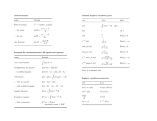
1. useful formulas
name formula
Euler’s formula ej θ
= cos(θ) + j sin(θ)
. . . for cosine cos(θ) =
ejθ
+ e−jθ
2
. . . for sine sin(θ) =
ejθ
− e−jθ
2 j
sinc function sinc(θ) :=
sin(π θ)
π θ
formulas for continuous-time LTI signals and systems
name formula
area under impulse
Z
δ(t) dt = 1
multiplication by impulse f(t) δ(t) = f(0) δ(t)
. . . by shifted impulse f(t) δ(t − to) = f(to) δ(t − to)
convolution f(t) ∗ g(t) =
Z
f(τ) g(t − τ) dτ
. . . with an impulse f(t) ∗ δ(t) = f(t)
. . . with a shifted impulse f(t) ∗ δ(t − to) = f(t − to)
transfer function H(s) =
Z
h(t) e−st
dt
frequency response Hf
(ω) =
Z
h(t) e−jωt
dt
. . . their connection Hf
(ω) = H(jω)
provided jω-axis ⊂ ROC
selected Laplace transform pairs
x(t) X(s) ROC
x(t)
Z
x(t) e−st
dt (def.)
δ(t) 1 all s
u(t)
1
s
Re(s) > 0
e−a t
u(t)
1
s + a
Re(s) > −a
cos(ωot) u(t)
s
s2 + ω2
o
Re(s) > 0
sin(ωot) u(t)
ωo
s2 + ω2
o
Re(s) > 0
e−a t
cos(ωot) u(t)
s + a
(s + a)2 + ω2
o
Re(s) > −a
e−a t
sin(ωot) u(t)
ωo
(s + a)2 + ω2
o
Re(s) > −a
Note: a is assumed real.
Laplace transform properties
x(t) X(s)
a x(t) + b g(t) a X(s) + b G(s)
x(t) ∗ g(t) X(s) G(s)
dx(t)
dt
s X(s)
x(t − to) e−s to
X(s)

2. selected Fourier transform pairs
x(t) Xf
(ω)
x(t)
Z
x(t) e−jωt
dt (def.)
1
2π
Z
Xf
(ω) ejωt
dω Xf
(ω)
δ(t) 1
1 2 π δ(ω)
u(t) π δ(ω) +
1
jω
ejωot
2 π δ(ω − ωo)
cos(ωo t) π δ(ω + ωo) + π δ(ω − ωo)
sin(ωo t) j π δ(ω + ωo) − j π δ(ω − ωo)
ωo
π
sinc
“ωo
π
t
”
ideal LPF
cut-off frequency ωo
symmetric pulse
2
ω
sin
„
T
2
ω
«
width T, height 1
impulse train impulse train
period T, height 1 period, height ωo =
2π
T
Fourier transform properties
x(t) Xf
(ω)
a x(t) + b g(t) a Xf
(ω) + b Gf
(ω)
x(a t)
1
|a|
X
“ω
a
”
x(t) ∗ g(t) Xf
(ω) Gf
(ω)
x(t) g(t)
1
2π
Xf
(ω) ∗ Gf
(ω)
x(t − to) e−jtoω
X(ω)
x(t) ejωot
X(ω − ωo)
x(t) cos(ωot) 0.5 X(ω + ωo) + 0.5 X(ω − ωo)
x(t) sin(ωot) j 0.5 X(ω + ωo) − j 0.5 X(ω − ωo)
dx(t)
dt
j ω Xf
(ω)