1. 1
Two-Dimensional Problems Using Constant Strain Triangles
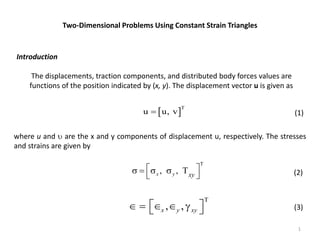
Introduction
The displacements, traction components, and distributed body forces values are
functions of the position indicated by (x, y). The displacement vector u is given as
T
u u, v
(1)
where u and are the x and y components of displacement u, respectively. The stresses
and strains are given by
T
, ,
x y xy
(2)
T
, ,
x y xy
(3)
2. 2
Fig. 1 shows a two-dimensional problem in a general setting. The body force, traction
vector, and elemental volume are given by
y
x t = thickness at (x, y)
fx, fy = body force components
per unit volume at (x, y)
Fig. 1 Two – dimensional problem
3. 3
f = [fx , fy] T T = [Tx , Ty]T and dV = t dA (4)
where t is the thickness along the z direction. The body force f has the units force/unit
volume, while the traction force T has the units, force/unit area. The strain-displacement
relations are given by
T
u v u v
, ,
x y y x
(5)
Stress and strains are related by
D
(6)
4. 4
Finite Element Modeling
The two- dimensional region is divided into straight-sided triangles. Fig.2 shows a typical
triangulation.
Fig. 2 Finite element discretization
5. 5
As seen from the numbering scheme used in trusses, the displacement components of
node j are taken as Q2j-1 in the x direction and Q2j in the y direction. The global
displacement vector is denoted as
Q = [Q1, Q2… QN] T (7)
where N is the number of degrees of freedom.
Computationally, the information on the triangulation is to be represented in the form
of nodal coordinates and connectivity.
7. 7
The displacement components of a local node j in Fig. 3 are represented as q2j-1 and q2j
in the x and y directions, respectively. The element displacement vector is denoted as
q = [q1, q2…, q6] T (8)
Fig.3 Triangular element.
8. 8
Constant – Strain Triangle (CST)
The displacements at points inside an element are represented in term of the nodal
displacement of the element. For the constant strain triangle, the shape functions are
linear over the element. The three shape functions N1, N2 and N3 corresponding to nodes
1, 2, and 3, respectively, are shown in Fig.4. In particular, N1+ N2+N3 represents a plan at a
height of 1 at nodes 1, 2, and 3, and, thus, it is parallel to the triangle 123.
N1+ N2+N3 = 1 (9)
N1, N2 and N3 are therefore not linearly independent; only two of these are independent.
The independent shape functions are conveniently represented by the pair ,.
N1 = N2 = N3 = 1- - (10)
9. 9
where , are natural coordinates (Fig.4).
The shape functions can be physically represented by area coordinates. A point (x, y)
in a triangle divides it into three areas, A1, A2, and A3, as shown in Fig.5. The shape
functions N1, N2 and N3 are precisely represented by
Fig. 4 Shape functions.
10. 10
Fig. 5 Area coordinates
1 2 3
1 2 3
A A A
N N N
A A A
(11)
where A is the area of the element. Clearly, N1+ N2+N3 = 1 at every point inside the
triangle.
11. 11
Isoparametric Representation
The displacements inside the element are now written using the shape functions and
the nodal values of the unknown displacement field.
1 1 2 3 3 5
1 2 2 4 3 6
u N q N q N q
N q N q N q
(12a)
or, using Eq.10
1 5 3 5 5
2 6 4 6 6
u q q q q q
q q q q q
(12b)
The relations 12a can be expressed in a matrix form by defining a shape function matrix
1 3
1 2 3
0 0
=
0 0 0
2
N 0 N N
N N N
N (13)
and
u = Nq (14)
12. 12
The coordinates can be interpolated as
1 1 2 2 3 3
1 2 2 2 3 3
x N x N x N x
y N y N y N y
(15a)
Substituting for N1, N2 and N3 = (1 – N1 – N2)
1 3 2 3 3
1 3 2 3 3
x x x x x x
y y y y y y
(15b)
Using the notation, x- and y- coordinates to the - and - coordinates. Equation 12
expresses u and as functions of and .
13. 13
Example 1
Evaluate the shape functions N1, N2 and N3 at the interior point P for the triangular
element shown in Fig.E1
Fig. E 1 Examples 1 and 2
14. 14
Solution Using the isoperametric representation (Eqs. 15), we have
3.85 = 1.5N1+ 7N2+4N3 = 2.5 + 3 +4
4.8 = 2N1+ 3.5N2+7N3 = 5 3.5+7
These two equations are arranged in the form
2.5 3 0.15
5 3.5 2.2
Solving the equations, we obtain = 0.3 and = 0.2, which implies that
N1 = 0.3 N2 = 0.2 N3 = 0.5
15. 15
( ( , ), ( , ))
u u x y
( ( , ), ( , ))
v v x y
In evaluating the strains, partial derivatives of u and are to be taken with
and similarly
Using the chain rule for partial derivatives of u, we have
respect to x and y.
u u x u y
x y
u u x u y
x y
which can be written in matrix notation as
u x y u
x
u
u x y
y
(16)
16. 16
Where the (2 X 2) square matrix is denoted as the Jacobian of the transformation, J:
x y
x y
J
(17)
On taking the derivative of x and y,
13 13
23 23
x y
x y
J (18)
17. 17
Also, from Eq.16
1
u
u
x
u u
y
J (19)
Where J-1 is the inverse of the Jacobian J, given by
23 13
1
23 13
1
det
y y
x x
J
J
(20)
13 23 23 13
det x y x y
J (21)
The magnitude of det J is twice the area of the triangle.
1
2 det
A J (22)
18. 18
Example 2
Determine the Jacobian of the transformation J for the triangular element shown in Fig.
E 1.
Solution We have
13 13
2 3 2 3
2.5 5.0
3.0 3.5
x y
x y
J
Thus, det J = 23.75 units. This is twice the area of the triangle. If 1, 2, 3 are in a clockwise
order, then det J will be negative.
From Eqs. 19 and 20, it follows that
23 13
23 13
1
det
u u
u
y y
x
u u u
x x
y
J
(23a)
19. 19
Replacing u by the displacement , we get a similar expression
23 13
23 13
v v
v
1
v v v
det
y y
x
x x
y
J
(23b)
Using the strain – displacement relations (5) and Eqs. 12 b and 23, we get
v
v
u
x
y
u
y x
20. 20
23 1 5 13 3 5
23 2 6 13 4 6
23 1 5 13 3 5 23 2 6 13 4 6
( ) ( )
1
( ) ( )
det
( ) ( ) ( ) ( )
y q q y q q
x q q x q q
x q q x q q y q q y q q
J
(24a)
From the definition of xij and yij, we can write y31 = y13 and y12 = y13 – y23, and so on.
The foregoing equation can be written in the form
23 1 31 3 12 5
32 2 13 4 21 6
32 1 23 2 13 3 31 4 21 5 12 6
1
det
y q y q y q
x q x q x q
x q y q x q y q x q y q
J
(24b)
This equation can be written in matrix form as
= Bq (25)
21. 21
where B is a (3 x 6) element strain-displacement matrix relating the three strains to the
six nodal displacements and is given by
23 31 12
32 13 21
32 23 13 31 21 12
0 0 0
1
0 0 0
det
y y y
x x x
x y x x x y
B
J
(26)
It may be noted that all the elements of the B matrix are constants expressed in terms of
the nodal coordinates.
Example 3
Find the strain –nodal displacement matrices Be for the elements shown in Fig. E 3. Use
local number given at the corners.
Fig. E 3
22. 22
Solution We have
23 31 12
32 13 21
32 23 13 31 21 12
0 0 0
1
0 0 0
det
y y y
x x x
x y x x x y
1
B
J
2 0 0 0 2 0
1
0 3 0 3 0 0
6
3 2 3 0 0 2
Potential-Energy Approach
The potential energy of the system, , is given by
T T T T
1
f
2
i i
i
A A L
t dA t dA t d
D u u u P
(27)
23. 23
T T T T
1
2
i i
L
e e i
e e
t dA t dA t d
D u f u T u P
(28a)
or
T T T
e i i
e e i
e L
U t dA t d
u f u T u P
(28b)
Element Stiffness
Now substitute for the strain from the element strain-displacement relationship in Eq. 5
into the element strain energy Ue in Eq.28b. to obtain
T
T T
1
2
1
2
e e
e
U t dA
t dA
D
q B DBq
(29a)
24. 24
Taking the element thickness te as constant over the element and remembering that all
terms in the D and B matrices are constants, we have
T T
1
2 t
e e e
U dA
q B DB q (29b)
Now, e
e
dA A
, where Ae is the area of the element. Thus,
T T
1
2
e e e
U t A
q B DBq (29c)
or
T
1
2
e
e
U q K q (29d)
25. 25
where Ke is the element stiffness matrix given by
ke = te Ae BTDB (30)
T
T
1
2
1
2
e
e
U q k q
= Q KQ
(31)
Force Terms
The body force term
T
e
t dA
u f appearing in the total potential energy in Eq. 28
is considered first. We have
T
( v )
e x y
e e
t dA t uf f dA
u f
26. 26
Using the interpolation relations given in Eq.12a, we find that
T
1 1 2 1
3 2 4 2
5 3 6 3
e x e y
e e e
e x e y
e e
e x e y
e e
t dA q t f N dA q t f N dA
q t f N dA q t f N dA
q t f N dA q t f N dA
u f
(32)
1
e
N dA
1
3
From the definition of shape functions on triangle, shown in Fig.4,
represents the volume of a tetrahedron with base area Ae and height of corner
equal to 1 (non dimensional). The volume of this tetrahedron is given by
(Base area) (Height) (Fig.6) as in
1
3
i e
e
N dA A
(33)
27. 27
Similarly, 1
2 3 3 ,
e
e e
N dA N dA A
Equation 32 can now be written in the form
T T e
e
t dA
u f q f (34)
where fe is the element body force vector, given as
T
, , , , ,
3
e e e
x y x y x y
t A
f f f f f f
f (35)
1 1
1 3 3
1 1 1 1
1
1 1 3
0 0 0 0
. .
det 2 .
e e
e
e e
e
N dA A h A
or N dA N Jd d A d d A
Fig. 6 Integral of a shape function.
28. 28
1 2
,
x y
T T
A traction force is a distributed load acting on the surface of the body. Consider
an edge , acted on by a traction in units of force per unit surface area,
shown in Fig. 7a. we have
1 2
T
u v
x y
L
td T T t d
u T (36)
Using the interpolations relation involving the shape functions
1 1 2 3
1 2 2 4
1 1 2 2
1 1 2 2
u
v
x x x
y y y
N q N q
N q N q
T N T N T
T N T N T
(37)
30. 30
and noting that
1 2 1 2 1 2
2 2
1 1 2 2 1 2 1 2 1 2
2 2
1 2 2 1 2 1
1 1 1
, ,
3 3 6
( ) ( )
N d N d N N d
x x y y
(38)
we get
1 2
T
1 2 3 4
, , , e
t d q q q q
u T T (39)
where Te is given by
1 2
1 2 1 2 1 2 1 2
2 ,2 , 2 , 2
6
T
e e
x x y y x x y y
t
T T T T T T T T
T (40)
If p1 and p2 are pressures acting normal to the line directed to the right as we move
from 1 to 2, as shown in Fig. 7b, then
1 1 2 2 1 1 2 2
, , ,
x x y y
T cp T cp T sp T sp
Where
1 2
1 2
( )
x x
s
and 1 2
1 2
( )
y y
c
31. 31
Example 4
A two-dimensional plate is shown in the Fig.E4. Determine the equivalent point loads at
nodes 7, 8, and 9 for the linearly distributed pressure load acting on the edge 7-8-9.
Fig. E 4
32. 32
Solution We consider the two edges 7-8 and 8-9 separately and then merge them.
For edge 7-8
p1 = 1MPa, p2 = 2MPa, x1 = 100mm, y1 = 20 mm, x2 =85 mm, y2 = 40mm,
2 2
1 2 1 2 1 2
( ) ( ) 25
x x y y mm
2 1 1 2
1 2 1 2
0.8, 0.6
y y x x
c s
1 1 1 1 2 2
0.8, 0.6, 1.6,
x y x c
T p c T p s T p
1 2
T
1
1 2 1 2 1 2 1 2
T
1.2
10 25
2 ,2 , 2 , 2
6
133.3, 100, 166.7, 125
y
x x y y x x y y
T p s
T T T T T T T T
T
N
33. 33
These loads add to F13, F14, F15, and F16, respectively.
For edge 8-9
p1 = 2MPa, p2 = 3MPa, x1 = 85mm, y1 = 40 mm, x2 =70 mm, y2 = 60mm,
2 2
1 2 1 2 1 2
( ) ( ) 25
x x y y mm
2 1 1 2
1 2 1 2
0.8, 0.6
y y x x
c s
1 1 1 1 2 2
1.6, 1.2, 2.4,
x y x
T p c T p s T p c
34. 34
These loads ad to F15, F16, F17, and F18, respectively. Thus,
[F13 F14 F15 F16 F17 F18] = [ 133.3 100 400 300 266.7 200] N
2 2
T
2
1 2 1 2 1 2 1 2
T
1.8
10 25
2 ,2 , 2 , 2
6
233.3, 175, 266.7, 200
y
x x y y x x y y
T p s
T T T T T T T T
T
N
Stress Calculations
Since strains are constant in a constant-strain triangle (CST) element, the
corresponding stresses are constant.
DBq
(41)
35. 35
Example 5
For the two-dimensional loaded plate shown in Fig.E.5,determine the displacements of
nodes 1 and 2 and the element stresses using plane stress conditions. Body force may be
neglected in comparison with the external forces.
Thickness t = 0.5 in.,
E = 30 X 106 psi, = 0.25
Fig. E 5
36. 36
Solution
For plane stress conditions, the material property matrix is given by
7 7
7 7
2
7
1 0 3.2X10 0.8X10 0
1 0 0.8X10 3.2X10 0
1
1 0 0 1.2X10
0 0
2
v
E
D v
v
v
Using the local numbering pattern used in Fig.E3, we establish the connectivity as
follows:
Nodes
Element No. 1 2 3
1 1 2 4
2 3 4 2
37. 37
On performing the matrix multiplication DBe, we get
1 7
1.067 0.4 0 0.4 1.067 0
10 0.267 1.6 0 1.6 0.267 0
0.6 0.4 0.6 0 0 0.4
DB
and
2 7
1.067 0.4 0 0.4 1.067 0
10 0.267 1.6 0 1.6 0.267 0
0.6 0.4 0.6 0 0 0.4
DB
These two relationships are used later in calculating stresses using σ e = DBeq.
The multiplication
T
e e
e e
t A B DB gives the element stiffness matrices,
39. 39
1
7
2
3
0.983 0.45 0.2 0
10 0.45 0.983 0 0
0.2 0 1.4 1000
Q
Q
Q
Solving for Q1, Q3, and Q4, we get
Q1 = 1.913 (10-5) in. Q3 = 0.875 (10-5) in. Q4 = –7.436 (10-5) in.
For element 1, the element nodal displacement vector is given by
q1 = 10-5 [1.913, 0, 0.0875, –7.436, 0, 0] T
The element stresses σ1 are calculated from DB1q as
σ1 = [–93.3, –1138.7, –62.3] T psi
Similarly,
q2 = 10-5 [0, 0, 0, 0, 0.875, –7.436] T
σ2 = [93.4, 23.4, –297.4] T psi
40. 40
Temperature Effects
If the distribution of the change in temperature ∆ T (x, y) is known, the strain due
to this change in temperature can be treated as an initial strain 0 .
T
0 [ , , 0]
T T
(42)
for plane stress and
T
0 (1 ) [ , , 0]
v T T
(43)
The stresses and strains are related by
0
( )
D
(44)
41. 41
The effect of temperature can be accounted for by considering the strain energy term.
T
0 0
1
2
U t dA
D
T T T
0 0 0
1
2
2
t dA
D D D
(45)
The first term in the previous expansion gives the stiffness matrix derived earlier. The
last term is a constant, which has no effect on the minimization process. The middle
term, which yields the temperature load, is now considered in detail. Using the strain
displacement relationship ,
Bq
T T
0 0
( )
T
e e
A
e
tdA t A
D q B D
(46)
42. 42
Example 6
Consider the two-dimensional loaded plate shown in Fig.E4. In addition to the conditions
there is an increase in temperature of the plate of 800 F. The coefficient of linear
expansion of the material α is 7 x 10⁻⁶/oF. Determine the additional displacements due
to temperature. Also, calculate the stresses in element 1.
Solution
We have 6 o 0
7X10 / F and 80 F. So
T
4
0
5.6
10 5.6
0 0
T
T
43. 43
Thickness t equals 0.5, and the area of the element A is 3 in2. The element
temperature loads are
1 1 T
0
( )
t A
DB
where DB1 is calculated in the solution. On evaluation, we get
T
1 T
( ) 11206 16800 0 16800 11206 0
with associated dofs 1, 2, 3, 4, 7, 8, and
T
2 T
( ) 11206 16800 0 16800 11206 0
with associated dofs 5, 6, 7, 8, 3, and 4.
44. 44
Picking the forces for dofs 1, 3, and 4 from the previous equations, we have
T
1 3 4 11206 11206 16800
F F F
F
On solving KQ = F, we get
3 3 3
1 3 4 1.862x10 1.992x10 0.934x10 in
Q Q Q
The displacements of element 1 due to temperature are
T
1 3 4 3
1.862x10 0 1.992x10 0.934x10 0 0
q
The stresses are calculated as
1 1 T 1
0
( )
DB q D
45. 45
On substituting for the terms on the right-hand side, we get
T
1 4
10 1.204 2.484 0.78 psi
We note that the displacements and stresses just calculated are due to temperature
change.
Fig. 8 Rectangular plate.
47. 47
Q2i moves along n as seen in Fig.10 and θ is the angle of inclination of n with respect to x-
axis, we have
2 1 2
sin cos 0
i i
Q Q
(47)
This boundary condition is seen to be a multipoint constraint. Using the penalty
approach presented this amounts to adding a term to the potential energy as in
T T 2
2 1 2
1 1
( sin cos )
2 2
i i
C Q Q
Q KQ Q F (48)
where C is a large number.
The squared term in Eq.48 can be written in the from
2
2 1
2
1 1
2 1 2 2 1 2
2 2 2
2
sin sin cos
( sin cos ) [ , ]
sin cos cos
i
i i i i
i
Q
C C
C Q Q Q Q
Q
C C
(49)
The terms 2
sin
C sin cos
C
, and
2
cos
C get added to the global stiffness
matrix.
48. 48
Orthotropic Materials
Denote 1, 2, and 3 as the principal material axes that are normal to the planes of
symmetry. The generalized Hooke’s law as referred to coordinate system 1,2,3 can be
written as *
31
21
1 1 2 3 23 23
1 2 3 23
32
12
2 1 2 3 13 13
1 2 3 13
13 23
3 1 2 3 12 12
1 2 3 12
1 1
,
1 1
,
1 1
,
v
v
E E E G
v
v
E E E G
v v
E E E G
(50)
49. 49
Where E1, E2, and E3 are the Young’s moduli along the principal material axes and G23,
G13, and G12 are the shear moduli that characterize changes of angles between
principal directions 2 and 3, 1 and 3, and 1 and 2, respectively. Due to symmetry of
Eqs.50, the following relations obtain:
1 21 2 12 2 32 3 23 3 13 1 31
, , ,
E v E v E v E v E v E v
(51)
Neglecting the z-component stresses
21 12
1 1 2 2 1 2 12 12
1 2 1 2 12
1 1 1
, ,
E E E E G
(52)
These equations can be inverted to express stress in terms of strain as
50. 50
1 1 21
12 21 12 21
1 1
2 12 2
2 2
12 21 12 21
12 12
12
0
1 1
0
1 1
0 0
E E v
v v v v
E v E
v v v v
G
(53)
Dm is symmetric since E1v21 = E2 v12.
A transformation matrix T is introduced as
2 2
2 2
2 2
cos sin 2sin cos
sin cos 2sin cos
sin cos sin cos cos sin
T
(54)
51. 51
The relations between the stresses (strains) in the material coordinate system and the
global coordinate system are
1 1
2 2
1 1
12 12
2 2
,
x x
y y
xy xy
T T (55)
Fig. 11 Orientation of material axes with respect to global axes; is the counterclockwise
angle from x-axis. Note: = 330o is equivalent to = 30o.
52. 52
The important relation we need is the D matrix, which relates stress and strain in the
global system as
11 12 13
12 22 23
13 23 33
x x
y y
xy xy
D D D
D D D
D D D
(56)
It can be shown* that the D matrix is related to the Dm matrix as
4 2 2 4
11 11 12 33 22
2 2 4 4
12 11 22 33 12
3 3
13 11 12 33 12 22 33
4 2 2 4
22 11 12 33 22
cos 2( )sin cos sin
( 4 )sin cos (sin cos )
( 2 )sin cos ( 2 )sin cos
sin 2( 2 )sin cos cos
m m m m
m m m m
m m m m m m
m m m m
D D D D D
D D D D D
D D D D D D D
D D D D D
D
3 3
23 11 12 33 12 22 33
2 2 4 4
33 11 22 12 33 33
( 2 )sin cos ( 2 )sin cos
( 2 2 )sin cos (sin cos )
m m m m m m
m m m m m
D D D D D D
D D D D D D
(57)