This document provides a list of errata for the textbook "Digital Signal Processing: A Computer-Based Approach" by Sanjit K. Mitra. It contains 22 corrections for Chapter 2, ranging from fixing equation numbers and variables to correcting program code. Similar corrections are provided for Chapters 3 through 7, with over 100 total errata listed to improve the accuracy of the textbook.

1. SOLUTIONS MANUAL
to accompany
Digital Signal Processing:
A Computer-Based Approach
Second Edition
Sanjit K. Mitra
Prepared by
Rajeev Gandhi, Serkan Hatipoglu, Zhihai He, Luca Lucchese,
Michael Moore, and Mylene Queiroz de Farias
1

2. Errata List
of
"Digital Signal Processing: A Computer-Based Approach", Second Edition
Chapter 2
1. Page 48, Eq. (2.17): Replace "y[n]" with "xu[n]".
2. Page, 51: Eq. (2.24a): Delete "
1
2
x[n] + x *[N − n]( )". Eq. (2.24b): Delete
"
1
2
x[n] − x *[N − n]( )".
3. Page 59, Line 5 from top and line 2 from bottom: Replace "− cos (ω1 + ω2 − π)n( )" with
"cos (2π – ω1 – ω2 )n( )".
4. Page 61, Eq. (2.52): Replace "A cos (Ωo + k ΩT )t + φ( )" with "A cos ±(Ωot + φ) + k ΩTt( )".
5. Page 62, line 11 from bottom: Replace "ΩT > 2Ωo " with "ΩT > 2 Ωo ".
6. Page 62, line 8 from bottom: Replace "2πΩo / ωT " with "2πΩo / ΩT ".
7. Page 65, Program 2_4, line 7: Replace "x = s + d;" with "x = s + d';".
8. Page 79, line 5 below Eq. (2.76): Replace " α
n
n=0
∞
∑ " with " α
n
n=0
∞
∑ ".
9. Page 81, Eq. (2.88): Replace "αL+1λ2
n
+ αNλN−L
n
" with "αL+1λ2
n
+L + αNλN− L
n
".
10. Page 93, Eq. (2.116): Replace the lower limit "n=–M+1" on all summation signs with "n=0".
11. Page 100, line below Eq. (2.140) and caption of Figure 2.38: Replace "ωo = 0.03 " with
"ωo = 0.06π ".
12. Page 110, Problem 2.44: Replace "{y[n]} = −1, −1, 11, −3, −10, 20, −16{ }" with
"{y[n]} = −1, −1, 11, −3, 30, 28, 48{ }", and
"{y[n]} = −14 − j5, −3 − j17, −2 + j5, −26 + j22, 9 + j12{ }" with
"{y[n]} = −14 − j5, −3 − j17, −2 + j5, −9.73 + j12.5, 5.8 + j5.67{ }".
13. Page 116, Exercise M2.15: Replace "randn" with "rand".
Chapter 3
1. Page 118, line 10 below Eq. (3.4): Replace "real" with "even".
2

3. 2. Page 121, Line 5 below Eq. (3.9): Replace " α
n
n=0
∞
∑ " with " α
n
n=0
∞
∑ ".
3. Page 125, Eq. (3.16): Delete the stray α.
4. Page 138, line 2 below Eq. (3.48): Replace "frequency response" with "discrete-time Fourier
transform".
5. Page 139, Eq. (3.53): Replace "x(n + mN)" with "x[n + mN]".
6. Page 139, lin2 2, Example 3.14: Replace "x[n] = 0 1 2 3 4 5{ }" with
"{x[n]} = 0 1 2 3 4 5{ }".
7. Page 139, line 3, Example 3.14: Replace "x[n]" with "{x[n]}", and "πk/4" with "2πk/4".
8. Page 139, line 6 from bottom: Replace "y[n] = 4 6 2 3 4 6{ }" with
"{y[n]} = 4 6 2 3{ }".
9. Page 141, Table 3.5: Replace "N[g < −k >N ]" with "N g[< −k >N ]".
10. Page 142, Table 3.7: Replace "argX[< −k >N ]" with "– argX[< −k >N ]".
11. Page 147, Eq. (3.86): Replace "
1 1 1 1
1 j −1 −j
1 −1 1 −1
1 −j −1 j












" with "
1 1 1 1
1 −j −1 j
1 −1 1 −1
1 j −1 −j












".
12. Page 158, Eq.(3.112): Replace " αn
n =−∞
−1
∑ z−n
" with "− αn
n=−∞
−1
∑ z−n
".
13. Page 165, line 4 above Eq. (3.125); Replace "0.0667" with "0.6667".
14. Page 165, line 3 above Eq. (3.125): Replace "10.0000" with "1.000", and "20.0000" with
"2.0000".
15. Page 165, line above Eq. (3.125): Replace "0.0667" with "0.6667", "10.0" with "1.0", and
"20.0" with "2.0".
16. Page 165, Eq. (3.125): Replace "0.667" with "0.6667".
17. Page 168, line below Eq. (3.132): Replace "z > λl " with " z > λl ".
18. Page 176, line below Eq. (3.143): Replace "R h " with "1/R h ".
19. Page 182, Problem 3.18: Replace "X(e− jω/2
)" with "X(−ejω/2
)".
3

4. 20. Page 186, Problem 3.42, Part (e): Replace "argX[< −k >N ]" with "– argX[< −k >N ]".
21. Page 187, Problem 3.53: Replace "N-point DFT" with "MN-point DFT", replace
"0 ≤ k ≤ N − 1" with "0 ≤ k ≤ MN − 1", and replace "x[< n >M]" with "x[< n >N ]".
22. Page 191, Problem 3.83: Replace " lim
n→∞
" with " lim
z→∞
".
23. Page 193, Problem 3.100: Replace "
P(z)
D' (z)
" with "−λl
P(z)
D' (z)
".
24. Page 194, Problem 3.106, Parts (b) and (d): Replace " z < α " with " z > 1 / α ".
25. page 199, Problem 3.128: Replace "(0.6)µ
[n]" with "(0.6)n
µ[n]", and replace "(0.8)µ
[n]"
with "(0.8)n
µ[n]".
26. Page 199, Exercise M3.5: Delete "following".
Chapter 4
1. Page 217, first line: Replace "ξN " with "ξM ".
2. Page 230, line 2 below Eq. (4.88): Replace "θg(ω) " with "θ(ω)".
3. Page 236, line 2 below Eq. (4.109): Replace "decreases" with "increases".
4. Page 246, line 4 below Eq. (4.132): Replace "θc(e
jω
)" with "θc(ω)".
5. Page 265, Eq. (4.202): Replace "1,2,K,3" with "1,2,3".
6. Page 279, Problem 4.18: Replace " H(e
j0
) " with " H(e
jπ/4
) ".
7. Page 286, Problem 4.71: Replace "z3 = − j0.3" with "z3 = −0.3 ".
8. Page 291, Problem 4.102: Replace
"H(z) =
0.4 + 0.5z
−1
+1.2 z
−2
+1.2z
−3
+ 0.5z
−4
+ 0.4 z
−5
1 + 0.9z−2
+ 0.2 z−4
" with
"H(z) =
0.1 + 0.5z
−1
+ 0.45z
−2
+ 0.45z
−3
+ 0.5z
−4
+ 0.1z
−5
1+ 0.9 z−2
+ 0.2z−4
".
9. Page 295, Problem 4.125: Insert a comma "," before "the autocorrelation".
Chapter 5
1. Page 302, line 7 below Eq. (5.9): Replace "response" with "spectrum".
4

5. 2. Page 309, Example 5.2, line 4: Replace "10 Hz to 20 Hz" with "5 Hz to 10 Hz". Line 6:
Replace "5k + 15" with "5k + 5". Line 7: Replace "10k + 6" with "5k + 3", and replace
"10k – 6" with "5(k+1) – 3".
3. Page 311, Eq. (5.24): Replace "Ga(jΩ − 2k(∆Ω)) " with "Ga(j(Ω − 2k(∆Ω))) ".
4. Page 318, Eq. (5.40): Replace "H(s)" with "Ha(s)", and replace "" with "".
5. Page 321, Eq. (5.54): Replace "" with "".
6. Page 333, first line: Replace "Ωp1" with " ˆΩ p1", and " Ωp2 " with " ˆΩ p2 ".
7. Page 349, line 9 from bottom: Replace "1/T" with "2π/T".
8. Page 354, Problem 5.8: Interchange "Ω1" and "Ω2".
9. Page 355, Problem 5.23: Replace "1 Hz" in the first line with "0.2 Hz".
10. Page 355, Problem 5.24: Replace "1 Hz" in the first line with "0.16 Hz".
Chapter 6
1. Page 394, line 4 from bottom: Replace "alpha1" with "fliplr(alpha1)".
2. Page 413, Problem 6.16: Replace
"H(z) = b0 + b1 z
−1
+ b2z
−1
z
−1
+ b3z
−1
1 +L+ bN−1z
−1
(1 + bNz
−1
)( )( )


 " with
"H(z) = b0 + b1z
−1
1 + b2z
−1
z
−1
+ b3z
−1
1 +L+ bN−1z
−1
(1 + bNz
−1
)( )( )


 ".
3. Page 415, Problem 6.27: Replace "H(z) =
3z
2
+ 18.5z+ 17.5
(2 z +1)(z + 2)
" with
"H(z) =
3z
2
+ 18.5z+ 17.5
(z + 0.5)(z + 2)
".
4. Page 415, Problem 6.28: Replace the multiplier value "0.4" in Figure P6.12 with "–9.75".
5. Page 421, Exercise M6.1: Replace "−7.6185z
−3
" with "−71.6185z
−3
".
6. Page 422, Exercise M6.4: Replace "Program 6_3" with "Program 6_4".
7. Page 422, Exercise M6.5: Replace "Program 6_3" with "Program 6_4".
8. Page 422, Exercise M6.6: Replace "Program 6_4" with "Program 6_6".
5

6. Chapter 7
1. Page 426, Eq. (7.11): Replace "h[n – N]" with "h[N – n]".
2. Page 436, line 14 from top: Replace "(5.32b)" with "(5.32a)".
3. Page 438, line 17 from bottom: Replace "(5.60)" with "(5.59)".
4. Page 439, line 7 from bottom: Replace "50" with "40".
5. Page 442, line below Eq. (7.42): Replace "F
−1
(ˆz) " with "1 / F(ˆz) ".
6. Page 442, line above Eq. (7.43): Replace "F
−1
(ˆz) " with "F(ˆz) ".
7. Page 442, Eq. (7.43): Replace it with "F(ˆz) = ±
ˆz − αl
1 − αl
*ˆz






l=1
L
∏ ".
8. Page 442, line below Eq. (7.43): Replace "where αl " with "where αl ".
9. Page 446, Eq. (7.51): Replace "β(1− α)" with "β(1+ α)".
10. Page 448, Eq. (7.58): Replace "ωc < ω ≤ π " with "ωc < ω ≤ π".
11. Page 453, line 6 from bottom: Replace "ωp − ωs " with "ωs − ωp ".
12. Page 457, line 8 from bottom: Replace "length" with "order".
13. Page 465, line 5 from top: Add "at ω = ωi " before "or in".
14. Page 500, Problem 7.15: Replace "2 kHz" in the second line with "0.5 kHz".
15. Page 502, Problem 7.22: Replace Eq. (7.158) with "Ha (s) =
Bs
s2
+ Bs + Ω0
2
".
16. Page 502, Problem 7.25: Replace "7.2" with "7.1".
17. Page 504, Problem 7.41: Replace "Hint(e
jω
) = e
− jω
" in Eq. (7.161) with
"Hint(e
jω
) =
1
jω
".
18. Page 505, Problem 7.46: Replace "16" with "9" in the third line from bottom.
19. Page 505, Problem 7.49: Replace "16" with "9" in the second line.
20. Page 510, Exercise M7.3: Replace "Program 7_5" with "Program 7_3".
21. Page 510, Exercise M7.4: Replace "Program 7_7" with "M-file impinvar".
22. Page 510, Exercise M7.6: Replace "Program 7_4" with "Program 7_2".
23. Page 511, Exercise M7.16: Replace "length" with "order".
6

7. 24. Page 512, Exercise M7.24: Replace "length" with "order".
Chapter 8
1. Page 518, line 4 below Eq. (6.7): Delete "set" before "digital".
2. Page 540, line 3 above Eq. (8.39): Replace "G[k]" with " X0[k]" and " H[k]" with " X1[k]".
Chapter 9
1. Page 595, line 2 below Eq. (9.30c): Replace "this vector has" with "these vectors have".
2. Page 601, line 2 below Eq. (9.63): Replace "2
b
" with "2
−b
".
3. Page 651, Problem 9.10, line 2 from bottom: Replace "
akz +1
1 + akz





 " with "
akz +1
z + ak





 ".
4. Page 653, Problem 9.15, line 7: Replace "two cascade" with "four cascade".
5. Page 653, Problem 9.17: Replace "A2(z) =
d1d2 + d1z
−1
+ z
−2
1 + d1z−1
+ d1d2z−2
" with
"A2(z) =
d2 + d1z
−1
+ z
−2
1 + d1z−1
+ d2z−2
".
6. Page 654, Problem 9.27: Replace "structure" with "structures".
7. Page 658, Exercise M9.9: Replace "alpha" with "α".
Chapter 10
1. Page 692, Eq. (10.57b): Replace "P0(α1) = 0.2469" with "P0(α1) = 0.7407".
2. Page 693, Eq. (10.58b): Replace "P0(α2) = –0.4321" with "P0(α2) = –1.2963 ".
3. Page 694, Figure 10.38(c): Replace "P−2(α0 )" with "P1(α0) ", "P−1(α0 )" with "P0(α0)",
"P0(α0)" with "P−1(α0 )", "P1(α0) " with "P−2(α0 )", "P−2(α1)" with "P1(α1)",
"P−1(α1)" with "P0(α1) ", "P0(α1) " with "P−1(α1)", "P1(α1)" with "P−2(α1)",
"P−2(α2) " with "P1(α2) ", "P−1(α2 )" with "P0(α2)", "P0(α2)" with "P−1(α2 )", and
"P−1(α2 )" with "P−2(α2) ".
4. Page 741, Problem 10.13: Replace "2.5 kHz" with "1.25 kHz".
5. Page 741, Problem 10.20: Replace " z
i
i=0
N
∑ " with " z
i
i=0
N−1
∑ ".
7

8. 6. Page 743, Problem 10.28: Replace "half-band filter" with a "lowpass half-band filter with a
zero at z = –1".
7. Page 747, Problem 10.50: Interchange "Y k " and "the output sequence y[n]".
8. Page 747, Problem 10.51: Replace the unit delays "z−1
" on the right-hand side of the structure
of Figure P10.8 with unit advance operators "z".
9. Page 749, Eq. (10.215): Replace "3H2
(z) − 2H2
(z)" with "z−2
3H2
(z) − 2H2
(z)[ ]".
10. Page 751, Exercise M10.9: Replace "60" with "61".
11. Page 751, Exercise M10.10: Replace the problem statement with "Design a fifth-order IIR
half-band Butterworth lowpass filter and realize it with 2 multipliers".
12. Page 751, Exercise M10.11: Replace the problem statement with "Design a seventh-order
IIR half-band Butterworth lowpass filter and realize it with 3 multipliers".
Chapter 11
1. Page 758, line 4 below Figure 11.2 caption: Replace "grid" with "grid;".
2. age 830, Problem 11.5: Insert "ga (t) = cos(200πt) " after "signal" and delete
"= cos(200πn) ".
3. Page 831, Problem 11.11: Replace "has to be a power-of-2" with "= 2
l
, where l is an
integer".
8

9. Chapter 2 (2e)
2.1 (a) u[n] = x[n]+ y[n]= {3 5 1 −2 8 14 0}
(b) v[n]= x[n]⋅w[n] = {−15 −8 0 6 −20 0 2}
(c) s[n] = y[n]− w[n] = {5 3 −2 −9 9 9 −3}
(d) r[n] = 4.5y[n] ={0 31.5 4.5 −13.5 18 40.5 −9}
2.2 (a) From the figure shown below we obtain
x[n]
y[n]
v[n] v[n–1]
z
–1
α
β
γ
v[n]= x[n]+ α v[n −1] and y[n] = βv[n −1]+ γ v[n −1]= (β + γ)v[n −1]. Hence,
v[n −1]= x[n −1]+ αv[n − 2] and y[n −1]= (β + γ)v[n − 2]. Therefore,
y[n] = (β + γ)v[n −1] = (β + γ)x[n −1]+ α(β + γ)v[n − 2] = (β + γ)x[n −1]+ α(β + γ)
y[n− 1]
(β+ γ)
= (β + γ)x[n −1]+ α y[n −1].
(b) From the figure shown below we obtain
x[n]
y[n]
z
–1
α β γ
z
–1
z
–1
z
–1
x[n–1] x[n–2]
x[n–3]x[n–4]
y[n] = γ x[n − 2]+ β x[n −1]+ x[n − 3]( )+ α x[n]+ x[n − 4]( ).
(c) From the figure shown below we obtain
v[n]
x[n] y[n]
z
–1
z
–1 v[n–1]
–1
d1
6

10. v[n]= x[n]− d1v[n− 1] and y[n] = d1v[n] + v[n− 1]. Therefore we can rewrite the second
equation as y[n] = d1 x[n]− d1v[n −1]( )+ v[n−1] = d1x[n]+ 1− d1
2
( )v[n −1] (1)
= d1x[n] + 1− d1
2
( ) x[n−1]− d1v[n − 2]( ) = d1x[n] + 1− d1
2
( )x[n −1]− d1 1− d1
2
( )v[n− 2]
From Eq. (1), y[n −1]= d1x[n− 1]+ 1− d1
2
( )v[n − 2], or equivalently,
d1y[n −1] = d1
2
x[n −1]+ d1 1− d1
2
( )v[n − 2]. Therefore,
y[n]+ d1y[n −1] = d1x[n]+ 1− d1
2
( )x[n− 1]− d1 1− d1
2
( )v[n − 2]+ d1
2
x[n −1] + d1 1− d1
2
( )v[n − 2]
= d1x[n] + x[n− 1], or y[n] = d1x[n]+ x[n −1]− d1y[n −1].
(d) From the figure shown below we obtain
v[n]
x[n] y[n]
v[n–1]
–1
d1
z
–1
z
–1 v[n–2]
d2
u[n]w[n]
v[n]= x[n]− w[n], w[n] = d1v[n −1]+ d2u[n], and u[n] = v[n − 2]+ x[n]. From these equations
we get w[n] = d2x[n]+ d1x[n −1]+ d2x[n − 2] − d1w[n− 1]− d2w[n − 2]. From the figure we also
obtain y[n] = v[n − 2] + w[n]= x[n − 2]+ w[n]− w[n − 2], which yields
d1y[n −1] = d1x[n − 3]+ d1w[n −1]− d1w[n − 3], and
d2y[n − 2]= d2x[n − 4]+ d2w[n − 2]− d2w[n − 4], Therefore,
y[n]+ d1y[n −1]+ d2y[n− 2] = x[n − 2]+ d1x[n− 3]+ d2x[n− 4]
+ w[n] + d1w[n− 1]+ d2w[n − 2]( )− w[n − 2]+ d1w[n− 3] + d2w[n − 4]( )
= x[n − 2] + d2x[n] + d1x[n −1] or equivalently,
y[n] = d2x[n]+ d1x[n −1] + x[n− 2]− d1y[n −1] − d2y[n− 2].
2.3 (a) x[n]= {3 −2 0 1 4 5 2}, Hence, x[−n] ={2 5 4 1 0 −2 3}, − 3 ≤ n ≤ 3.
Thus, xev [n] =
1
2
(x[n]+ x[−n]) = {5 / 2 3 / 2 2 1 2 3/ 2 5 / 2}, − 3≤ n ≤ 3, and
xod[n] =
1
2
(x[n] − x[−n]) = {1 / 2 −7 / 2 −2 0 2 7 / 2 −1 / 2}, − 3≤ n ≤ 3.
(b) y[n] = {0 7 1 −3 4 9 −2}. Hence, y[−n] ={−2 9 4 −3 1 7 0}, − 3≤ n ≤ 3.
Thus, yev[n] =
1
2
(y[n]+ y[−n]) = {−1 8 5 / 2 −3 5 / 2 8 −1}, − 3 ≤ n ≤ 3, and
yod[n] =
1
2
(y[n] − y[−n]) = {1 −1 −3/ 2 0 1 3 / 2 −1}, − 3≤ n ≤ 3.
7

11. (c) w[n]= {−5 4 3 6 −5 0 1}, Hence, w[−n] = {1 0 −5 6 3 4 −5}, − 3 ≤ n ≤ 3.
Thus, wev[n]=
1
2
(w[n] + w[−n]) = {−2 2 −1 6 −1 2 −2}, − 3 ≤ n ≤ 3, and
wod[n] =
1
2
(w[n]− w[−n]) = {−3 2 4 0 −4 −2 3}, − 3≤ n ≤ 3,
2.4 (a) x[n] = g[n]g[n]. Hence x[−n] = g[−n]g[−n]. Since g[n] is even, hence g[–n] = g[n].
Therefore x[–n] = g[–n]g[–n] = g[n]g[n] = x[n]. Hence x[n] is even.
(b) u[n] = g[n]h[n]. Hence, u[–n] = g[–n]h[–n] = g[n](–h[n]) = –g[n]h[n] = –u[n]. Hence
u[n] is odd.
(c) v[n] = h[n]h[n]. Hence, v[–n] = h[n]h[n] = (–h[n])(–h[n]) = h[n]h[n] = v[n]. Hence
v[n] is even.
2.5 Yes, a linear combination of any set of a periodic sequences is also a periodic sequence and
the period of the new sequence is given by the least common multiple (lcm) of all periods.
For our example, the period = lcm(N1,N2 ,N3 ). For example, if N1 = 3, N2 = 6, and N3 =12,
then N = lcm(3, 5, 12) = 60.
2.6 (a) xpcs[n] =
1
2
{x[n] + x *[−n]} =
1
2
{Aαn
+ A *(α*)−n
}, and
xpca[n] =
1
2
{x[n]− x *[−n]} =
1
2
{Aαn
− A *(α*)−n
}, −N ≤ n ≤ N.
(b) h[n]= {−2 + j5 4 − j3 5 + j6 3 + j −7 + j2} −2 ≤ n ≤ 2 , and hence,
h *[−n]= {−7 − j2 3 − j 5 − j6 4 + j3 −2 − j5}, −2 ≤ n ≤ 2. Therefore,
hpcs[n] =
1
2
{h[n] + h*[−n]} ={−4.5 + j1.5 3.5 − j2 5 3.5+ j2 −4.5 − j1.5} and
hpca[n] =
1
2
{h[n] − h*[−n]}= {2.5+ j3.5 0.5− j j6 −0.5 − j −2.5+ j3.5} −2 ≤ n ≤ 2.
2.7 (a) x[n]{ }= Aα
n
{ } where A and α are complex numbers, with α < 1.
Since for n < 0, α
n
can become arbitrarily large hence {x[n]} is not a bounded sequence.
(b) y[n]{ }= Aα
n
µ[n] where A and α are complex numbers, with α <1.
In this case y[n] ≤ A ∀n hence {y[n]} is a bounded sequence.
(c) h[n]{ } = Cβ
n
µ[n] where C and β are complex numbers,with β > 1.
Since β
n
becomes arbitrarily large as n increases hence {h[n]} is not a bounded sequence.
8

12. (d) {g[n]} = 4sin(ωan). Since − 4≤ g[n]≤ 4 for all values of n, {g[n]} is a bounded
sequence.
(e) {v[n]} = 3cos2
(ωbn2
). Since − 3≤ v[n] ≤ 3 for all values of n, {v[n]} is a bounded
sequence.
2.8 (a) Recall, xev[n] =
1
2
x[n]+ x[−n]( ).
Since x[n] is a causal sequence, thus x[–n] = 0 ∀n > 0 . Hence,
x[n] = xev[n]+ xev[−n] = 2xev[n], ∀n > 0 . For n = 0, x[0] = xev[0].
Thus x[n] can be completely recovered from its even part.
Likewise, xod[n]=
1
2
x[n]– x[−n]( ) =
1
2
x[n], n > 0,
0, n = 0.




Thus x[n] can be recovered from its odd part ∀n except n = 0.
(b) 2yca[n] = y[n]− y*[−n]. Since y[n] is a causal sequence y[n] = 2yca[n] ∀n > 0.
For n = 0, Im{y[0]} = yca[0]. Hence real part of y[0] cannot be fully recovered from yca[n].
Therefore y[n] cannot be fully recovered from yca[n].
2ycs[n] = y[n]+ y*[−n]. Hence, y[n] = 2ycs[n] ∀n > 0 .
For n = 0, Re{y[0]} = ycs[0]. Hence imaginary part of y[0] cannot be recovered from ycs[n].
Therefore y[n] cannot be fully recovered from ycs[n].
2.9 xev[n] =
1
2
x[n]+ x[−n]( ). This implies, xev[–n]=
1
2
x[–n]+ x[n]( ) = xev[n].
Hence even part of a real sequence is even.
xod[n]=
1
2
x[n]– x[–n]( ). This implies, xod[–n]=
1
2
x[–n]– x[n]( ) = –xod[n].
Hence the odd part of a real sequence is odd.
2.10 RHS of Eq. (2.176a) is xcs[n]+ xcs[n − N] =
1
2
x[n] + x*[−n]( ) +
1
2
x[n − N] + x*[N − n]( ).
Since x[n] = 0 ∀n < 0 , Hence
xcs[n]+ xcs[n − N] =
1
2
x[n] + x*[N − n]( ) = xpcs[n], 0 ≤ n ≤ N –1.
RHS of Eq. (2.176b) is
xca[n]+ xca[n− N]=
1
2
x[n]− x*[−n]( )+
1
2
x[n − N]− x*[n− N]( )
=
1
2
x[n]− x *[N − n]( ) = xpca[n], 0 ≤ n ≤ N –1.
9

13. 2.11 xpcs[n]=
1
2
x[n]+ x*[< −n >N ]( ) for 0 ≤ n ≤ N –1, Since, x[< −n >N ] = x[N − n], it follows
that xpcs[n]=
1
2
x[n]+ x*[N − n]( ), 1≤ n ≤ N –1.
For n = 0, xpcs[0] =
1
2
x[0]+ x*[0]( ) = Re{x[0]}.
Similarly xpca[n] =
1
2
x[n]− x*[< −n >N ]( ) =
1
2
x[n]− x *[N − n]( ), 1≤ n ≤ N –1. Hence,
for n = 0, xpca[0] =
1
2
x[0]− x *[0]( ) = jIm{x[0]}.
2.12 (a) Given x[n]
n=−∞
∞
∑ < ∞. Therefore, by Schwartz inequality,
x[n]
2
n=−∞
∞
∑ ≤ x[n]
n=−∞
∞
∑





 x[n]
n=−∞
∞
∑





 < ∞.
(b) Consider x[n] =
1/ n, n ≥1,
0, otherwise.{ The convergence of an infinite series can be shown
via the integral test. Let an = f(x), where f(x) is a continuous, positive and decreasing
function for all x ≥ 1. Then the series ann =1
∞
∑ and the integral f(x)dx
1
∞
∫ both converge or
both diverge. For an = 1/ n, f(x) = 1/n. But
1
x
dx
1
∞
∫ = lnx( )1
∞
= ∞ − 0 = ∞. Hence,
x[n]n =−∞
∞
∑ = 1
nn=1
∞
∑ does not converge, and as a result, x[n] is not absolutely
summable. To show {x[n]} is square-summable, we observe here an =
1
n2 , and thus,
f(x) =
1
x2 . Now,
1
x2 dx
1
∞
∫ = −
1
x






1
∞
= −
1
∞
+
1
1
= 1. Hence,
1
n2n =1
∞
∑ converges, or in other
words, x[n] = 1/n is square-summable.
2.13 See Problem 2.12, Part (b) solution.
2.14 x2[n] =
cosωcn
πn
, 1≤ n ≤ ∞. Now,
cosωcn
πn






2
n=1
∞
∑ ≤
1
π2n2n=1
∞
∑ . Since,
1
n2n=1
∞
∑ =
π2
6
,
cosωcn
πn






2
n=1
∞
∑ ≤
1
6
. Therefore x2[n] is square-summable.
Using integral test we now show that x2[n] is not absolutely summable.
cosωcx
πx1
∞
∫ dx =
1
π
⋅
cosωcx
x
cosωcx
x⋅cosint(ωcx)
1
∞
where cosint is the cosine integral function.
Since
cosωcx
πx1
∞
∫ dx diverges,
cosωcn
πnn=1
∞
∑ also diverges.
10

14. 2.15 x
2
[n]
n=−∞
∞
∑ = xev[n] + xod[n]( )2
n=−∞
∞
∑
= xev
2
[n]
n=−∞
∞
∑ + xod
2
[n]
n= −∞
∞
∑ + 2 xev[n]xod[n]
n=−∞
∞
∑ = xev
2
[n]
n= −∞
∞
∑ + xod
2
[n]
n=−∞
∞
∑
as xevn= –∞
∞
∑ [n]xod[n] = 0 since xev [n]xod[n] is an odd sequence.
2.16 x[n] = cos(2πkn / N), 0 ≤ n ≤ N –1. Hence,
Ex = cos
2
(2πkn / N)
n=0
N−1
∑ =
1
2
1+ cos(4πkn / N)( )
n =0
N −1
∑ =
N
2
+
1
2
cos(4πkn / N)
n=0
N −1
∑ .
Let C = cos(4πkn / N)
n=0
N−1
∑ , and S = sin(4πkn / N)
n =0
N−1
∑ .
Therefore C + jS = ej4πkn/ N
n=0
N−1
∑ =
e
j4πk
− 1
e
j4πk / N
− 1
= 0. Thus, C = Re C + jS{ } = 0 .
As C = Re C + jS{ } = 0 , it follows that Ex =
N
2
.
2.17 (a) x1[n] = µ[n]. Energy = µ2
[n]n =−∞
∞
∑ = 12
n=−∞
∞
∑ = ∞.
Average power = lim
K→∞
1
2K + 1
(µ[n])2
n=−K
K
∑ = lim
K→∞
1
2K +1
12
n =0
K
∑ = lim
K→∞
K
2K + 1
=
1
2
.
(b) x2 [n]= nµ[n]. Energy = nµ[n]( )n =−∞
∞
∑
2
= n2
n=−∞
∞
∑ = ∞.
Aveerage power = lim
K→∞
1
2K + 1
(nµ[n])2
n=−K
K
∑ = lim
K→∞
1
2K + 1
n2
n=0
K
∑ = ∞.
(c) x3[n] = Aoe
jωo n
. Energy = Aoe
jωo n
n =−∞
∞
∫
2
= Ao
2
n =−∞
∞
∑ = ∞. Average power =
lim
K→∞
1
2K + 1
Aoe
jωon 2
n=−K
K
∑ = lim
K→∞
1
2K +1
Aon =−K
K
∑
2
= lim
K→∞
2K Ao
2
2K + 1
= Ao
2
.
(d) x[n]= Asin
2πn
M
+ φ





 = Aoe
jωon
+ A1e
−jωon
, where ωo =
2π
M
, Ao = −
A
2
ejφ
and
A1 =
A
2
e− jφ
. From Part (c), energy = ∞ and average power = Ao
2
+ A1
2
+ 4Ao
2
A1
2
=
3
4
A2
.
2.18 Now, µ[n] =
1, n ≥ 0,
0, n < 0.



Hence, µ[−n − 1]=
1, n < 0,
0, n ≥ 0.



Thus, x[n] = µ[n] + µ[−n −1].
2.19 (a) Consider a sequence defined by x[n] = δ[k]
k =−∞
n
∑ .
11

15. If n < 0 then k = 0 is not included in the sum and hence x[n] = 0, whereas for n ≥ 0 , k = 0 is
included in the sum hence x[n] = 1 ∀ n ≥ 0 . Thus x[n] = δ[k]
k =−∞
n
∑ =
1, n ≥ 0,
0, n < 0,



= µ[n].
(b) Since µ[n]=
1, n ≥ 0,
0, n < 0,



it follows that µ[n –1] =
1, n ≥ 1,
0, n ≤ 0.



Hence, µ[n] –µ[n −1]=
1, n = 0,
0, n ≠ 0,{ = δ[n].
2.20 Now x[n]= Asin ω0n + φ( ).
(a) Given x[n]= 0 − 2 −2 − 2 0 2 2 2{ }. The fundamental period is N = 4,
hence ωo = 2π / 8= π / 4. Next from x[0] = Asin(φ) = 0 we get φ = 0, and solving
x[1] = Asin(
π
4
+ φ) = Asin(π / 4) = − 2 we get A = –2.
(b) Given x[n] = 2 2 − 2 − 2{ }. The fundamental period is N = 4, hence
ω0 = 2π/4 = π/2. Next from x[0]= Asin(φ) = 2 and x[1]= Asin(π / 2 + φ) = A cos(φ) = 2 it
can be seen that A = 2 and φ = π/4 is one solution satisfying the above equations.
(c) x[n] = 3 −3{ }. Here the fundamental period is N = 2, hence ω0 = π. Next from x[0]
= A sin(φ) = 3 and x[1]= Asin(φ + π) = −A sin(φ) = −3 observe that A = 3 and φ = π/2 that A = 3
and φ = π/2 is one solution satisfying these two equations.
(d) Given x[n] = 0 1.5 0 −1.5{ }, it follows that the fundamental period of x[n] is N =
4. Hence ω0 = 2π / 4 = π / 2. Solving x[0]= Asin(φ) = 0 we get φ = 0, and solving
x[1] = Asin(π / 2) =1.5, we get A = 1.5.
2.21 (a) ˜x1[n] = e−j0.4πn
. Here, ωo = 0.4π. From Eq. (2.44a), we thus get
N =
2πr
ωo
=
2π r
0.4π
= 5r = 5 for r =1.
(b) ˜x2 [n]= sin(0.6πn + 0.6π). Here, ωo = 0.6π. From Eq. (2.44a), we thus get
N =
2πr
ωo
=
2π r
0.6π
=
10
3
r = 10 for r = 3.
(c) ˜x3[n] = 2cos(1.1πn − 0.5π) + 2sin(0.7πn). Here, ω1 = 1.1π and ω2 = 0.7π . From Eq.
(2.44a), we thus get N1 =
2π r1
ω1
=
2π r1
1.1π
=
20
11
r1 and N2 =
2πr2
ω2
=
2π r2
0.7π
=
20
7
r2 . To be periodic
12

16. we must have N1 = N2. This implies,
20
11
r1 =
20
7
r2 . This equality holds for r1 = 11 and r2 = 7,
and hence N = N1 = N2 = 20.
(d) N1 =
2π r1
1.3π
=
20
13
r1 and N2 =
2πr2
0.3π
=
20
3
r2 . It follows from the results of Part (c), N = 20
with r1 = 13 and r2 = 3.
(e) N1 =
2π r1
1.2π
=
5
3
r1 , N2 =
2πr2
0.8π
=
5
2
r2 and N3 = N2. Therefore, N = N1 = N2 = N2 = 5 for
r1 = 3 and r2 = 2.
(f) ˜x6[n]= n modulo 6. Since ˜x6[n + 6] = (n+6) modulo 6 = n modulo 6 = ˜x6[n].
Hence N = 6 is the fundamental period of the sequence ˜x6[n].
2.22 (a) ωo = 0.14π. Therefore, N =
2πr
ωo
=
2πr
0.14π
=
100
7
r =100 for r = 7.
(b) ωo = 0.24π. Therefore, N =
2πr
ωo
=
2πr
0.24π
=
25
3
r = 25 for r = 3.
(c) ωo = 0.34π. Therefore, N =
2πr
ωo
=
2πr
0.34π
=
100
17
r =100 for r = 17.
(d) ωo = 0.75π. Therefore, N =
2πr
ωo
=
2π r
0.75π
=
8
3
r = 8 for r = 3.
2.23 x[n]= xa(nT) = cos(ΩonT) is a periodic sequence for all values of T satisfying ΩoT ⋅ N = 2πr
for r and N taking integer values. Since, ΩoT = 2πr / N and r/N is a rational number, ΩoT
must also be rational number. For Ωo = 18 and T = π/6, we get N = 2r/3. Hence, the smallest
value of N = 3 for r = 3.
2.24 (a) x[n] = 3δ[n + 3]− 2δ[n + 2]+ δ[n] + 4δ[n −1]+ 5δ[n − 2]+ 2δ[n −3]
(b) y[n] = 7 δ[n+ 2]+ δ[n +1]− 3δ[n]+ 4δ[n− 1]+ 9δ[n − 2]− 2δ[n − 3]
(c) w[n] = −5δ[n + 2] + 4δ[n + 2]+ 3δ[n +1] + 6δ[n]− 5δ[n −1]+δ[n − 3]
2.25 (a) For an input xi [n], i = 1, 2, the output is
yi [n]= α1xi[n] + α2xi[n −1] + α3xi [n − 2] + α4xi[n − 4], for i = 1, 2. Then, for an input
x[n]= Ax1[n] + B x2[n],the output is y[n] = α1 A x1[n]+ Bx2[n]( ) + α2 A x1[n −1] + Bx2[n −1]( )
+α3 A x1[n − 2] + Bx2[n − 2]( ) + α4 Ax1[n − 3] + B x2[n − 3]( )
= A α1x1[n]+ α2x1[n −1] + α3x1[n − 2]+ α4x1[n − 4]( )
+ B α1x2[n] + α2x2[n − 1] + α3x2[n − 2] + α4x2[n − 4]( ) = A y1[n] + By2[n].
Hence, the system is linear.
13

17. (b) For an input xi [n], i = 1, 2, the output is
yi [n]= b0xi[n] + b1xi [n − 1]+ b2xi[n − 2] + a1yi [n − 1] + a2yi [n − 2], i = 1, 2. Then, for an
input x[n]= Ax1[n] + B x2[n],the output is
y[n] = A b0x1[n] + b1x1[n − 1]+ b2x1[n − 2] + a1y1[n −1] + a2y1[n − 2]( )
+ B b0x2[n] + b1x2 [n − 1] + b2x2[n − 2]+ a1y2[n −1] + a2y2[n − 2]( ) = A y1[n] + By2[n].
Hence, the system is linear.
(c) For an input xi [n], i = 1, 2, the output is yi [n]=,
xi[n / L], n = 0,± L, ± 2L, K
0, otherwise,



Consider the input x[n]= Ax1[n] + B x2[n], Then the output y[n] for n = 0,± L, ± 2L, K is
given by y[n] = x[n / L] = Ax1[n / L] + B x2[n / L]= A y1[n] + By2[n]. For all other values
of n, y[n] = A ⋅0 + B ⋅ 0 = 0. Hence, the system is linear.
(d) For an input xi [n], i = 1, 2, the output is yi [n]= xi[n / M]. Consider the input
x[n]= Ax1[n] + B x2[n], Then the output y[n] = Ax1[n / M] + B x2[n / M]= A y1[n] + B y2[n].
Hence, the system is linear.
(e) For an input xi [n], i = 1, 2, the output is yi [n]=
1
M
xi[n − k]k =0
M−1
∑ . Then, for an
input x[n]= Ax1[n] + B x2[n],the output is yi [n]=
1
M
Ax1[n − k] + Bx2[n − k]( )k =0
M−1
∑
= A
1
M
x1[n − k]k =0
M−1
∑





 + B
1
M
x2[n − k]k =0
M−1
∑





 = A y1[n] + By2[n]. Hence, the system is
linear.
(f) The first term on the RHS of Eq. (2.58) is the output of an up-sampler. The second
term on the RHS of Eq. (2.58) is simply the output of an unit delay followed by an up-
sampler, whereas, the third term is the output of an unit adavance operator followed by an
up-sampler We have shown in Part (c) that the up-sampler is a linear system. Moreover,
the delay and the advance operators are linear systems. A cascade of two linear systems is
linear and a linear combination of linear systems is also linear. Hence, the factor-of-2
interpolator is a linear system.
(g) Following thearguments given in Part (f), it can be shown that the factor-of-3
interpolator is a linear system.
2.26 (a) y[n] = n2x[n].
For an input xi[n] the output is yi[n] = n2xi[n], i = 1, 2. Thus, for an input x3[n] = Ax1[n]
+ Bx2[n], the output y3[n] is given by y3[n] = n2
A x1[n] + Bx2[n]( ) = A y1[n] + By2[n].
Hence the system is linear.
Since there is no output before the input hence the system is causal. However, y[n] being
proportional to n, it is possible that a bounded input can result in an unbounded output. Let
x[n] = 1 ∀ n , then y[n] = n2. Hence y[n] → ∞ as n → ∞ , hence not BIBO stable.
Let y[n] be the output for an input x[n], and let y1[n] be the output for an input x1[n]. If
x1[n]= x[n − n0 ] then y1[n] = n2
x1[n] = n2
x[n − n0 ]. However, y[n − n0 ] = (n − n0 )2
x[n − n0].
Since y1[n] ≠ y[n− n0 ], the system is not time-invariant.
14

18. (b) y[n] = x4
[n].
For an input x1[n] the output is yi[n] = xi
4[n], i = 1, 2. Thus, for an input x3[n] = Ax1[n] +
Bx2[n], the output y3[n] is given by y3[n] = (A x1[n] + Bx2[n])4
≠ A4
x1
4
[n]+ A4
x2
4
[n]
Hence the system is not linear.
Since there is no output before the input hence the system is causal.
Here, a bounded input produces bounded output hence the system is BIBO stable too.
Let y[n] be the output for an input x[n], and let y1[n] be the output for an input x1[n]. If
x1[n]= x[n − n0 ] then y1[n] = x1
4
[n]= x4
[n − n0] = y[n − n0 ]. Hence, the system is time-
invariant.
(c) y[n] = β + x[n − l]
l =0
3
∑ .
For an input xi[n] the output is yi [n]= β + xi[n − l ]
l =0
3
∑ , i = 1, 2. Thus, for an input x3[n] =
Ax1[n] + Bx2[n], the output y3[n] is given by
y[n] = β + A x1[n − l ]+ Bx2[n − l ]( )
l =0
3
∑ = β + A x1[n − l]
l =0
3
∑ + Bx2[n − l ]
l =0
3
∑
≠ A y1[n] + By2[n]. Since β ≠ 0 hence the system is not linear.
Since there is no output before the input hence the system is causal.
Here, a bounded input produces bounded output hence the system is BIBO stable too.
Also following an analysis similar to that in part (a) it is easy to show that the system is time-
invariant.
(d) y[n] = β + x[n − l ]
l =–3
3
∑
For an input xi[n] the output is yi [n]= β + xi [n − l]
l =–3
3
∑ , i = 1, 2. Thus, for an input x3[n] =
Ax1[n] + Bx2[n], the output y3[n] is given by
y[n] = β + A x1[n − l ] + Bx2[n − l ]( )
l =−3
3
∑ = β + A x1[n − l ]
l =−3
3
∑ + Bx2[n − l ]
l =−3
3
∑
≠ A y1[n] + By2[n]. Since β ≠ 0 hence the system is not linear.
Since there is output before the input hence the system is non-causal.
Here, a bounded input produces bounded output hence the system is BIBO stable.
15

19. Let y[n] be the output for an input x[n], and let y1[n] be the output for an input x1[n]. If
x1[n]= x[n − n0 ] then y1[n] = β + x1[n − l ]
l =–3
3
∑ = β + x1[n − n0 − l ]
l =–3
3
∑ = y[n − n0]. Hence the
system is time-invariant.
(e) y[n] = αx[−n]
The system is linear, stable, non causal. Let y[n] be the output for an input x[n] and y1[n]
be the output for an input x1[n]. Then y[n] = αx[−n] and y1[n] = α x1[−n].
Let x1[n]= x[n − n0 ], then y1[n] = α x1[−n] = α x[−n − n0 ], whereas y[n − n0 ]= αx[n0 − n].
Hence the system is time-varying.
(f) y[n] = x[n – 5]
The given system is linear, causal, stable and time-invariant.
2.27 y[n] = x[n + 1] – 2x[n] + x[n – 1].
Let y1[n] be the output for an input x1[n] and y2[n] be the output for an input x2[n]. Then
for an input x3[n] = αx1[n]+βx2[n] the output y3[n] is given by
y3[n] = x3[n +1]− 2x3[n]+ x3[n −1]
= αx1[n +1]− 2αx1[n]+ αx1[n −1]+βx2[n +1]− 2βx2[n]+ βx2[n −1]
= αy1[n]+ βy2[n].
Hence the system is linear. If x1[n]= x[n − n0 ] then y1[n] = y[n− n0 ]. Hence the system is
time-inavariant. Also the system's impulse response is given by
h[n] =
−2,
1,
0,
n = 0,
n =1,-1,
elsewhere.




Since h[n] ≠ 0 ∀ n < 0 the system is non-causal.
2.28 Median filtering is a nonlinear operation. Consider the following sequences as the input to
a median filter: x1[n]= {3, 4, 5} and x2[n] ={2, − 2, − 2}. The corresponding outputs of the
median filter are y1[n] = 4 and y2[n]= −2. Now consider another input sequence x3[n] =
x1[n] + x2[n]. Then the corresponding output is y3[n] = 3, On the other hand,
y1[n] + y2 [n] = 2 . Hence median filtering is not a linear operation. To test the time-
invariance property, let x[n] and x1[n] be the two inputs to the system with correponding
outputs y[n] and y1[n]. If x1[n]= x[n − n0 ] then
y1[n] = median{x1[n − k],......., x1[n],.......x1[n+ k]}
= median{x[n − k − n0],......., x[n− n0],.......x[n + k − n0 ]}= y[n − n0 ].
Hence the system is time invariant.
16

20. 2.29 y[n] =
1
2
y[n −1]+
x[n]
y[n −1]






Now for an input x[n] = α µ[n], the ouput y[n] converges to some constant K as n → ∞.
The above difference equation as n → ∞ reduces to K =
1
2
K +
α
K





 which is equivalent to
K
2
= α or in other words, K = α .
It is easy to show that the system is non-linear. Now assume y1[n] be the output for an
input x1[n]. Then y1[n] =
1
2
y1[n −1]+
x1[n]
y1[n−1]








If x1[n]= x[n − n0 ]. Then, y1[n] =
1
2
y1[n −1]+
x[n − n0 ]
y1[n −1]







 .
Thus y1[n] = y[n− n0 ]. Hence the above system is time invariant.
2.30 For an input xi [n], i = 1, 2, the input-output relation is given by
yi [n]= xi[n] − yi
2
[n − 1]+ yi[n −1]. Thus, for an input Ax1[n] + Bx2[n], if the output is
Ay1[n] + By2[n], then the input-output relation is given by A y1[n]+ By2[n] =
A x1[n]+ Bx2 [n] − A y1[n − 1]+ By2[n −1]( )2
+ A y1[n −1] + By2[n − 1] = A x1[n]+ Bx2 [n]
− A2
y1
2
[n − 1]− B2
y2
2
[n − 1] + 2AB y1[n − 1]y2[n − 1]+ A y1[n −1] + By2[n − 1]
≠ A x1[n] − A2
y1
2
[n − 1] + Ay1[n − 1]+ B x2[n]− B2
y2
2
[n −1] + By2[n − 1]. Hence, the system
is nonlinear.
Let y[n] be the output for an input x[n] which is related to x[n] through
y[n] = x[n] − y2
[n −1] + y[n − 1]. Then the input-output realtion for an input x[n − no ] is given
by y[n − no ]= x[n − no ] − y2
[n − no − 1] + y[n − no − 1], or in other words, the system is time-
invariant.
Now for an input x[n] = α µ[n], the ouput y[n] converges to some constant K as n → ∞.
The above difference equation as n → ∞ reduces to K = α − K2
+ K , or K2
= α , i.e.
K = α .
2.31 As δ[n] = µ[n] − µ[n −1], Τ{δ[n]} = Τ{µ[n]}− Τ{µ[n −1]}⇒ h[n] = s[n] − s[n −1]
For a discrete LTI system
y[n] = h[k]x[n − k]
k =−∞
∞
∑ = s[k]−s[k −1]( )x[n − k]
k =−∞
∞
∑ = s[k]x[n − k]
k =−∞
∞
∑ − s[k −1]x[n − k]
k=−∞
∞
∑
2.32 y[n] = h[m]˜x[n − m]m=−∞
∞
∑ . Hence, y[n + kN]= h[m]˜x[n + kN − m]m=−∞
∞
∑
= h[m]˜x[n − m]m=−∞
∞
∑ = y[n]. Thus, y[n] is also a periodic sequence with a period N.
17

21. 2.33 Now δ[n − r] * δ[n − s] = δ[m − r]δ[n − s − m]m=−∞
∞
∑ = δ[n − r − s]
(a) y1[n] = x1[n] * h1[n] = 2δ[n − 1]− 0.5δ[n − 3]( ) * 2δ[n]+ δ[n − 1]− 3δ[n − 3]( )
= 4δ[n −1] * δ[n] – δ[n − 3] * δ[n] + 2δ[n −1] * δ[n −1] – 0.5 δ[n − 3] * δ[n −1]
– 6δ[n −1] * δ[n − 3] + 1.5 δ[n − 3] * δ[n − 3] = 4δ[n −1] – δ[n − 3] + 2δ[n −1]
– 0.5 δ[n − 4] – 6δ[n − 4] + 1.5δ[n − 6]
= 4δ[n −1] + 2δ[n −1] – δ[n − 3] – 6.5δ[n − 4] + 1.5δ[n − 6]
(b) y2 [n] = x2 [n] * h2[n] = −3δ[n −1] + δ[n + 2]( ) * −δ[n − 2] − 0.5δ[n −1] + 3δ[n − 3]( )
= − 0.5δ[n + 1]− δ[n] + 3δ[n − 1] + 1.5δ[n − 2] + 3δ[n − 3]− 9δ[n − 4]
(c) y3[n] = x1[n] * h2[n] =
2δ[n − 1]− 0.5δ[n − 3]( ) * −δ[n − 2] − 0.5δ[n −1] + 3δ[n − 3]( ) =
− δ[n − 2]− 2δ[n − 3]− 6.25δ[n − 4] + 0.5δ[n − 5] – 1.5δ[n − 6]
(d) y4 [n]= x2 [n] * h1[n] = −3δ[n −1] + δ[n + 2]( ) * 2δ[n]+ δ[n − 1]− 3δ[n − 3]( ) =
2 δ[n + 2]+ δ[n +1] − δ[n −1] − 3δ[n − 2] – 9δ[n − 4]
2.34 y[n] = g[m]h[n − m]m=N1
N2
∑ . Now, h[n – m] is defined for M1 ≤ n − m ≤ M2 . Thus, for
m = N1 , h[n–m] is defined for M1 ≤ n − N1 ≤ M2 , or equivalently, for
M1 + N1 ≤ n ≤ M2 + N1. Likewise, for m = N2 , h[n–m] is defined for M1 ≤ n − N2 ≤ M2 , or
equivalently, for M1 + N2 ≤ n ≤ M2 + N2 .
(a) The length of y[n] is M2 + N2 − M1 – N1 + 1.
(b) The range of n for y[n] ≠ 0 is min M1 + N1,M1 + N2( ) ≤ n ≤ max M2 + N1,M2 + N2( ), i.e.,
M1 + N1 ≤ n ≤ M2 + N2 .
2.35 y[n] = x1[n] * x2[n] = x1[n− k]x2[k]
k =−∞
∞
∑ .
Now, v[n] = x1[n – N1] * x2[n – N2] = x1[n − N1 − k]x2[k − N2 ]k =−∞
∞
∑ . Let
k− N2 = m. Then v[n] = x1[n − N1 − N2 − m]x2 [m]m=−∞
∞
∑ = y[n − N1 − N2 ],
2.36 g[n] = x1[n] * x2[n] * x3[n] = y[n] * x3[n] where y[n] = x1[n] * x2[n]. Define v[n] =
x1[n – N1] * x2[n – N2]. Then, h[n] = v[n] * x3[n – N3] . From the results of Problem
2.32, v[n] = y[n − N1 − N2 ]. Hence, h[n] = y[n − N1 − N2 ] * x3[n – N3] . Therefore,
using the results of Problem 2.32 again we get h[n] = g[n– N1– N2– N3] .
18

22. 2.37 y[n] = x[n] * h[n] = x[n − k]h[k]
k =−∞
∞
∑ . Substituting k by n-m in the above expression, we
get y[n] = x[m]h[n − m]
m=−∞
∞
∑ = h[n] * x[n]. Hence convolution operation is commutative.
Let y[n] = x[n] * h1[n]+ h2[n]( ) = = x[n − k] h1[k]+ h2[k]( )
k =−∞
∞
∑
= x[n − k]h1[k]+ x[n − k]h2[k]
k=−∞
k =∞
∑
k =−∞
∞
∑ = x[n] * h1[n] + x[n] * h2[n]. Hence convolution is
distributive.
2.38 x3[n] * x2[n] * x1[n] = x3[n] * (x2[n] * x1[n])
As x2[n] * x1[n] is an unbounded sequence hence the result of this convolution cannot be
determined. But x2[n] * x3[n] * x1[n] = x2[n] * (x3[n] * x1[n]) . Now x3[n] * x1[n] =
0 for all values of n hence the overall result is zero. Hence for the given sequences
x3[n] * x2[n] * x1[n] ≠ x2[n] * x3[n] * x1[n] .
2.39 w[n] = x[n] * h[n] * g[n]. Define y[n] = x[n] * h[n] = x[k]h[n − k]
k
∑ and f[n] =
h[n] * g[n] = g[k]h[n − k]
k
∑ . Consider w1[n] = (x[n] * h[n]) * g[n] = y[n] * g[n]
= g[m] x[k]h[n− m − k].
k
∑
m
∑ Next consider w2[n] = x[n] * (h[n] * g[n]) = x[n] * f[n]
= x[k] g[m]h[n− k − m].
m
∑
k
∑ Difference between the expressions for w1[n] and w2[n] is
that the order of the summations is changed.
A) Assumptions: h[n] and g[n] are causal filters, and x[n] = 0 for n < 0. This implies
y[m]=
0, form < 0,
x[k]h[m − k],
k =0
m
∑ form ≥ 0.




Thus, w[n] = g[m]y[n− m]
m=0
n
∑ = g[m] x[k]h[n − m − k]
k=0
n −m
∑m=0
n
∑ .
All sums have only a finite number of terms. Hence, interchange of the order of summations
is justified and will give correct results.
B) Assumptions: h[n] and g[n] are stable filters, and x[n] is a bounded sequence with
x[n] ≤ X. Here, y[m]= h[k]x[m − k]
k=−∞
∞
∑ = h[k]x[m − k]
k=k1
k2
∑ + εk1,k2
[m] with
εk1,k2
[m] ≤ εnX.
19

23. In this case all sums have effectively only a finite number of terms and the error can be
reduced by choosing k1 and k2 sufficiently large. Hence in this case the problem is again
effectively reduced to that of the one-sided sequences. Here, again an interchange of
summations is justified and will give correct results.
Hence for the convolution to be associative, it is sufficient that the sequences be stable and
single-sided.
2.40 y[n] = x[n − k]h[k]
k=−∞
∞
∑ . Since h[k] is of length M and defined for 0 ≤ k ≤ M –1, the
convolution sum reduces to y[n] = x[n− k]h[k]
k=0
(M−1)
∑ . y[n] will be non-zero for all those
values of n and k for which n – k satisfies 0 ≤ n − k ≤ N −1.
Minimum value of n – k = 0 and occurs for lowest n at n = 0 and k = 0. Maximum value
of n – k = N–1 and occurs for maximum value of k at M – 1. Thus n – k = M – 1
⇒ n = N + M − 2 . Hence the total number of non-zero samples = N + M – 1.
2.41 y[n] = x[n] * x[n] = x[n − k]x[k]
k =−∞
∞
∑ .
Since x[n – k] = 0 if n – k < 0 and x[k] = 0 if k < 0 hence the above summation reduces to
y[n] = x[n − k]x[k]
k =n
N −1
∑ =
n+ 1, 0≤ n ≤ N −1,
2N − n, N ≤ n ≤ 2N − 2.




Hence the output is a triangular sequence with a maximum value of N. Locations of the
output samples with values
N
4
are n =
N
4
– 1 and
7N
4
– 1. Locations of the output samples
with values
N
2
are n =
N
2
– 1 and
3N
2
– 1. Note: It is tacitly assumed that N is divisible by 4
otherwise
N
4
is not an integer.
2.42 y[n] = h[k]x[n − k]k=0
N−1
∑ . The maximum value of y[n] occurs at n = N–1 when all terms
in the convolution sum are non-zero and is given by
y[N − 1]= h[k] = kk =1
N
∑k =0
N−1
∑ =
N(N + 1)
2
.
2.43 (a) y[n] = gev[n] * hev[n] = hev[n − k]gev[k]
k=−∞
∞
∑ . Hence, y[–n] = hev[−n − k]gev[k]
k=−∞
∞
∑ .
Replace k by – k. Then above summation becomes
y[−n] = hev[−n + k]gev[−k]
k=−∞
∞
∑ = hev[−(n − k)]gev[−k]
k=−∞
∞
∑ = hev[(n − k)]gev[k]
k=−∞
∞
∑
= y[n].
Hence gev[n] * hev[n] is even.
20

24. (b) y[n] = gev[n] * hod[n] = hod[(n − k)]gev[k]
k=−∞
∞
∑ . As a result,
y[–n] = hod[(−n − k)]gev[k]
k=−∞
∞
∑ = hod[−(n − k)]gev[−k]
k=−∞
∞
∑ = − hod[(n − k)]gev[k]
k=−∞
∞
∑ .
Hence gev[n] * hod[n] is odd.
(c) y[n] = god[n] * hod[n] = hod[n − k]god[k]
k=−∞
∞
∑ . As a result,
y[–n] = hod[−n − k]god[k]
k=−∞
∞
∑ = hod[−(n − k)]god[−k]
k=−∞
∞
∑ = hod[(n − k)]god[k]
k=−∞
∞
∑ .
Hence god[n] * hod[n] is even.
2.44 (a) The length of x[n] is 7 – 4 + 1 = 4. Using x[n]=
1
h[0]
y[n] − h[k]x[n − k]k =1
7
∑{ },
we arrive at x[n] = {1 3 –2 12}, 0 ≤ n ≤ 3
(b) The length of x[n] is 9 – 5 + 1 = 5. Using x[n]=
1
h[0]
y[n] − h[k]x[n − k]k =1
9
∑{ }, we
arrive at x[n] = {1 1 1 1 1}, 0 ≤ n ≤ 4.
(c) The length of x[n] is 5 – 3 + 1 = 3. Using x[n]=
1
h[0]
y[n] − h[k]x[n − k]k =1
5
∑{ }, we get
x[n] = −4 + j, −0.6923 + j0.4615, 3.4556 + j1.1065{ }, 0 ≤ n ≤ 2.
2.45 y[n] = ay[n – 1] + bx[n]. Hence, y[0] = ay[–1] + bx[0]. Next,
y[1] = ay[0] + bx[1] = a
2
y[−1]+ a bx[0] + bx[1]. Continuing further in similar way we
obtain y[n] = an+1
y[−1]+ an−k
bx[k]
k =0
n
∑ .
(a) Let y1[n] be the output due to an input x1[n]. Then y1[n] = a
n +1
y[−1] + a
n−k
bx1[k]
k=0
n
∑ .
If x1[n] = x[n – n0 ] then
y1[n] = a
n +1
y[−1] + a
n−k
bx[k− n0 ]
k=n0
n
∑ = a
n+1
y[−1]+ a
n −n 0 −r
bx[r]
r=0
n −n 0
∑ .
However, y[n − n0 ] = a
n−n0 +1
y[−1]+ a
n−n0 −r
bx[r]
r=0
n−n0
∑ .
Hence y1[n] ≠ y[n− n0 ] unless y[–1] = 0. For example, if y[–1] = 1 then the system is time
variant. However if y[–1] = 0 then the system is time -invariant.
21

25. (b) Let y1[n] and y2[n] be the outputs due to the inputs x1[n] and x2[n]. Let y[n] be the output
for an input α x1[n]+ βx2[n]. However,
αy1[n]+ βy2[n]= αa
n+1
y[−1]+ βa
n+1
y[−1]+ α a
n −k
bx1[k]
k=0
n
∑ + β a
n −k
bx2[k]
k =0
n
∑
whereas
y[n] = a
n+1
y[−1]+ α a
n −k
bx1[k]
k =0
n
∑ + β a
n −k
bx2[k]
k =0
n
∑ .
Hence the system is not linear if y[–1] = 1 but is linear if y[–1] = 0.
(c) Generalizing the above result it can be shown that for an N-th order causal discrete time
system to be linear and time invariant we require y[–N] = y[–N+1] = L = y[–1] = 0.
2.46 ystep[n] = h[k]µ[n − k]k=0
n
∑ = h[k],k =0
n
∑ n ≥ 0, and ystep[n] = 0, n < 0. Since h[k] is
nonnegative, ystep[n] is a monotonically increasing function of n for n ≥ 0, and is not
oscillatory. Hence, no overshoot.
2.47 (a) f[n] = f[n – 1] + f[n – 2]. Let f[n] = αr
n
, then the difference equation reduces to
αr
n
− αr
n−1
− αr
n −2
= 0 which reduces to r
2
− r −1= 0 resulting in r =
1± 5
2
.
Thus, f[n]= α1
1+ 5
2






n
+ α2
1− 5
2






n
.
Since f[0] = 0 hence α1 + α2 = 0. Also f[1] = 1 hence
α1 + α2
2
+ 5
α1 −α2
2
= 1.
Solving for α1 and α2 , we get α1 = –α2 =
1
5
. Hence, f[n]=
1
5
1+ 5
2






n
−
1
5
1− 5
2






n
.
(b) y[n] = y[n – 1] + y[n – 2] + x[n – 1]. As system is LTI, the initial conditions are equal
to zero.
Let x[n] = δ[n]. Then, y[n] = y[n – 1] + y[n – 2] + δ[n −1]. Hence,
y[0] = y[– 1] + y[– 2] = 0 and y[1] = 1. For n > 1 the corresponding difference equation is
y[n] = y[n – 1] + y[n – 2] with initial conditions y[0] = 0 and y[1] = 1, which are the same as
those for the solution of Fibonacci's sequence. Hence the solution for n > 1 is given by
y[n] =
1
5
1+ 5
2






n
−
1
5
1− 5
2






n
Thus f[n] denotes the impulse response of a causal LTI system described by the difference
equation y[n] = y[n – 1] + y[n – 2] + x[n – 1].
2.48 y[n] = αy[n−1]+x[n]. Denoting, y[n] = yre[n] + j yim[n], and α = a + jb, we get,
yre[n]+ jyim[n] = (a + jb)(yre[n −1]+ jyim[n −1]) + x[n].
22

26. Equating the real and the imaginary parts , and noting that x[n] is real, we get
yre[n] = ayre[n −1]− byim[n −1]+ x[n], (1)
yim [n] = byre[n −1]+ ayim[n−1]
Therefore
yim [n −1] =
1
a
yim[n]−
b
a
yre[n −1]
Hence a single input, two output difference equation is
yre[n] = ayre[n −1]−
b
a
yim[n]+
b2
a
yre[n −1]+ x[n]
thus byim [n −1] = −ayre[n −1] +(a2
+ b2
)yre[n − 2]+ a x[n −1].
Substituting the above in Eq. (1) we get
yre[n] = 2a yre[n− 1]− (a2
+ b2
)yre[n − 2] + x[n]− a x[n −1]
which is a second-order difference equation representing yre[n] in terms of x[n].
2.49 From Eq. (2.59), the output y[n] of the factor-of-3 interpolator is given by
y[n] = xu[n] +
1
3
xu[n − 1]+ xu[n + 2]( ) +
2
3
xu[n − 2]+ xu[n +1]( ) where xu[n] is the output of
the factor-of-3 up-sampler for an input x[n]. To compute the impulse response we set x[n] =
δ[n], in which case, xu[n]= δ[3n]. As a result, the impulse response is given by
h[n]= δ[3n] +
1
3
δ[3n − 3] + δ[3n + 6]( )+
2
3
δ[3n − 6] + δ[3n + 3]( ) or
=
1
3
δ[n + 2] +
2
3
δ[n +1] + δ[n] +
1
3
δ[n − 1]+
2
3
δ[n − 2].
2.50 The output y[n] of the factor-of-L interpolator is given by
y[n] = xu[n] +
1
L
xu[n − 1]+ xu [n + L − 1]( ) +
2
L
xu[n − 2]+ xu[n + L − 2]( )
+K +
L − 1
L
xu[n − L + 1] + xu [n + 1]( ) where xu[n] is the output of the factor-of-L up-
sampler for an input x[n]. To compute the impulse response we set x[n] = δ[n], in which
case, xu[n]= δ[Ln]. As a result, the impulse response is given by
h[n]= δ[Ln]+
1
L
δ[Ln − L]+ δ[Ln + L(L − 1)]( ) +
2
L
δ[Ln − 2L] + δ[Ln + L(L − 2)]( )
+K +
L − 1
L
δ[Ln − L(L –1)] + δ[Ln + L]( ) =
1
L
δ[n + (L − 1)] +
2
L
δ[n + (L − 2)] +K
+
L −1
L
δ[n +1] + δ[n] +
1
L
δ[n − 1]+
2
L
δ[n − 2] +
L − 1
L
δ[n − (L − 1)]
2.51 The first-order causal LTI system is characterized by the difference equation
y[n] = p0 x[n]+ p1x[n −1]− d1y[n −1]. Letting x[n] = δ[n] we obtain the expression for its
impulse response h[n]= p0δ[n] + p1δ[n −1] − d1h[n −1]. Solving it for n = 0, 1, and 2, we get
h[0] = p0 , h[1]= p1 − d1h[0] = p1 − d1p0, and h[2] = −d1h[1] == −d1 p1 − d1p0( ). Solving these
equations we get p0 = h[0], d1 = −
h[2]
h[1]
, and p1 = h[1] −
h[2]h[0]
h[1]
.
23

27. 2.52 pkx[n − k] = dk y[n− k]
k=0
N
∑
k=0
M
∑ .
Let the input to the system be x[n] = δ[n]. Then, pkδ[n − k] = dk h[n− k]
k=0
N
∑
k=0
M
∑ . Thus,
pr = dkh[r − k]
k =0
N
∑ . Since the system is assumed to be causal, h[r – k] = 0 ∀ k > r.
pr = dkh[r − k]
k =0
r
∑ = h[k]dr−k
k =0
r
∑ .
2.53 The impulse response of the cascade is given by h[n] = h1[n] * h2[n] where
h1[n]= α
n
µ[n] and h2[n] = β
n
µ[n]. Hence, h[n] = α
k
β
n−k
k=0
n
∑







 µ[n].
2.54 Now, h[n] = α
n
µ[n]. Therefore y[n] = h[k]x[n− k]
k =−∞
∞
∑ = α
k
k =0
∞
∑ x[n − k]
= x[n]+ α
k
k =1
∞
∑ x[n− k] = x[n]+ α α
k
k =0
∞
∑ x[n −1− k] = x[n]+ αy[n− 1].
Hence, x[n] = y[n] – αy[n −1]. Thus the inverse system is given by y[n]= x[n] – αx[n −1].
The impulse response of the inverse system is given by g[n]= 1
↑
−α






.
2.55 y[n] = y[n −1] + y[n − 2] + x[n −1]. Hence, x[n – 1] = y[n] – y[n – 1] – y[n – 2], i.e.
x[n] = y[n + 1] – y[n] – y[n – 1]. Hence the inverse system is characterised by
y[n] = x[n + 1] – x[n] – x[n – 1] with an impulse response given by g[n] = 1 –1
↑
–1






.
2.56 y[n] = p0 x[n]+ p1x[n −1]− d1y[n −1] which leads to x[n] =
1
p0
y[n]+
d1
p0
y[n−1]−
p1
p0
x[n− 1]
Hence the inverse system is characterised by the difference equation
y1[n] =
1
p0
x1[n]+
d1
p0
x1[n −1]−
p1
p0
y1[n −1].
2.57 (a) From the figure shown below we observe
x[n] y[n]h1[n] h 2[n]
h3[n] h4 [n]
h 5[n]
v[n]
↓
24

28. v[n] = (h1[n] + h3[n] * h5[n]) * x[n] and y[n] = h2[n] * v[n] + h3[n] * h4[n] * x[n].
Thus, y[n] = (h2[n] * h1[n] + h2[n] * h3[n] * h5[n] + h3[n] * h4[n]) * x[n].
Hence the impulse response is given by
h[n] = h2[n] * h1[n] + h2[n] * h3[n] * h5[n] + h3[n] * h4[n]
(b) From the figure shown below we observe
x[n] y[n]h1[n ] h2[n] h 3[n]
h4[n]
h5[n]
v[n]
↓
v[n] = h4[n] * x[n] + h1[n] * h2[n] * x[n].
Thus, y[n] = h3[n] * v[n] + h1[n] * h5[n] * x[n]
= h3[n] * h4[n] * x[n] + h3[n] * h1[n] * h2[n] * x[n] + h1[n] * h5[n] * x[n]
Hence the impulse response is given by
h[n] = h3[n] * h4[n] + h3[n] * h1[n] * h2[n] + h1[n] * h5[n]
2.58 h[n] = h1[n] * h2[n]+ h3[n]
Now h1[n] * h2[n] = 2δ[n − 2] − 3δ[n + 1]( ) * δ[n − 1]+ 2δ[n + 2]( )
= 2δ[n − 2] * δ[n −1] – 3δ[n + 1] * δ[n −1] + 2δ[n − 2] * 2δ[n + 2]
– 3δ[n + 1] * 2δ[n + 2] = 2δ[n − 3] – 3δ[n] + 4 δ[n] – 6δ[n + 3]
= 2δ[n − 3] + δ[n] – 6δ[n + 3]. Therefore,
y[n] = 2δ[n − 3] + δ[n] – 6δ[n + 3] + 5δ[n − 5] + 7δ[n − 3] + 2δ[n −1] −δ[n] + 3δ[n + 1]
= 5δ[n − 5] + 9δ[n − 3] + 2δ[n −1] + 3δ[n + 1] − 6δ[n + 3]
2.59 For a filter with complex impulse response, the first part of the proof is same as that for a
filter with real impulse response. Since, y[n] = h[k]x[n − k]
k =−∞
∞
∑ ,
y[n] = h[k]x[n − k]
k=−∞
∞
∑ ≤ h[k]
k=−∞
∞
∑ x[n − k].
Since the input is bounded hence 0 ≤ x[n] ≤ Bx . Therefore, y[n] ≤ Bx h[k]
k=−∞
∞
∑ .
So if h[k]
k=−∞
∞
∑ = S < ∞ then y[n] ≤ BxS indicating that y[n] is also bounded.
25

29. To proove the converse we need to show that if a bounded output is produced by a bounded
input then S < ∞. Consider the following bounded input defined by x[n] =
h *[−n]
h[−n]
.
Then y[0]=
h*[k]h[k]
h[k]
k =−∞
∞
∑ = h[k]
k =−∞
∞
∑ = S. Now since the output is bounded thus S < ∞.
Thus for a filter with complex response too is BIBO stable if and only if h[k]
k=−∞
∞
∑ = S < ∞ .
2.60 The impulse response of the cascade is g[n] = h1[n] * h2[n] or equivalently,
g[k] = h1[k − r]h2[r]
r=–∞
∞
∑ . Thus,
g[k]
k=–∞
∞
∑ = h1[k – r]
r=–∞
∞
∑
k=–∞
∞
∑ h2[r] ≤ h1[k]
k=–∞
∞
∑







 h2[r]
r=–∞
∞
∑







 .
Since h1[n] and h2[n] are stable, h1[k]
k
∑ < ∞ and h2[k]
k
∑ < ∞ . Hence, g[k]
k
∑ < ∞.
Hence the cascade of two stable LTI systems is also stable.
2.61 The impulse response of the parallel structure g[n] = h1[n] + h2[n] . Now,
g[k]
k
∑ = h1[k] + h2[k]
k
∑ ≤ h1[k]
k
∑ + h2[k]
k
∑ . Since h1[n] and h2[n] are stable,
h1[k]
k
∑ < ∞ and h2[k]
k
∑ < ∞ . Hence, g[k]
k
∑ < ∞. Hence the parallel connection of
two stable LTI systems is also stable.
2.62 Consider a cascade of two passive systems. Let y1[n] be the output of the first system which is
the input to the second system in the cascade. Let y[n] be the overall output of the cascade.
The first system being passive we have y1[n]
2
n =−∞
∞
∑ ≤ x[n]
2
n=−∞
∞
∑ .
Likewise the second system being also passive we have y[n]
2
n =−∞
∞
∑ ≤ y1[n]
2
n =−∞
∞
∑ ≤ x[n]
2
n=−∞
∞
∑ ,
indicating that cascade of two passive systems is also a passive system. Similarly one can
prove that cascade of two lossless systems is also a lossless system.
2.63 Consider a parallel connection of two passive systems with an input x[n] and output y[n].
The outputs of the two systems are y1[n] and y2 [n], respectively. Now,
y1[n]
2
n =−∞
∞
∑ ≤ x[n]
2
n=−∞
∞
∑ , and y2[n]
2
n =−∞
∞
∑ ≤ x[n]
2
n=−∞
∞
∑ .
Let y1[n] = y2 [n]= x[n] satisfying the above inequalities. Then y[n] = y1[n]+ y2[n] = 2x[n]
and as a result, y[n]
2
n =−∞
∞
∑ = 4 x[n]
2
n =−∞
∞
∑ > x[n]
2
n =−∞
∞
∑ . Hence, the parallel
connection of two passive systems may not be passive.
26

30. 2.64 Let pkx[n − k]
k=0
M
∑ = y[n]+ dky[n − k]
k=1
N
∑ be the difference equation representing the causal
IIR digital filter. For an input x[n] = δ[n], the corresponding output is then y[n] = h[n], the
impulse response of the filter. As there are M+1 {pk} coefficients, and N {dk} coefficients,
there are a total of N+M+1 unknowns. To determine these coefficients from the impulse
response samples, we compute only the first N+M+1 samples. To illstrate the method, without
any loss of generality, we assume N = M = 3. Then , from the difference equation
reprsentation we arrive at the following N+M+1 = 7 equations:
h[0]= p0 ,
h[1]+ h[0]d1 = p1,
h[2]+ h[1]d1 + h[0]d2 = p2,
h[3]+ h[2]d1 + h[1]d2 + h[0]d3 = p3,
h[4]+ h[3]d1 + h[2]d2 + h[1]d3 = 0,
h[5]+ h[4]d1 + h[3]d2 + h[2]d3 = 0,
h[6]+ h[5]d1 + h[4]d2 + h[3]d3 = 0.
Writing the last three equations in matrix form we arrive at
h[4]
h[5]
h[6]








+
h[3] h[2] h[1]
h[4] h[3] h[2]
h[5] h[4] h[3]








d1
d2
d3










=
0
0
0








,
and hence,
d1
d2
d3










= –
h[3] h[2] h[1]
h[4] h[3] h[2]
h[5] h[4] h[3]








–1
h[4]
h[5]
h[6]








.
Substituting these values of {di} in the first four equations written in matrix form we get
p0
p1
p2
p3












=
h[0] 0 0 0
h[1] h[0] 0 0
h[2] h[1] h[0] 0
h[3] h[2] h[1] h[0]










1
d1
d2
d3












.
2.65 y[n] = y[−1] + x[l ]l =0
n
∑ = y[−1]+ l µ[l ]l =0
n
∑ = y[−1] + ll =0
n
∑ = y[−1]+
n(n + 1)
2
.
(a) For y[–1] = 0, y[n] =
n(n +1)
2
(b) For y[–1] = –2, y[n] = –2 +
n(n +1)
2
=
n2
+ n − 4
2
.
2.66 y(nT) = y (n –1)T( ) + x(τ)dτ
(n−1)T
nT
∫ = y (n –1)T( ) + T ⋅x (n –1)T( ). Therefore, the difference
equation representation is given by y[n] = y[n − 1]+ T ⋅ x[n − 1], where y[n] = y(nT) and
x[n]= x(nT).
27

31. 2.67 y[n] =
1
n
x[l ]l =1
n
∑ =
1
n
x[l ]l =1
n −1
∑ +
1
n
x[n], n ≥ 1. y[n − 1] =
1
n − 1
x[l ]l =1
n−1
∑ , n ≥ 1. Hence,
x[l ]l =1
n −1
∑ = (n − 1)y[n − 1]. Thus, the difference equation representation is given by
y[n] =
n − 1
n





 y[n −1] +
1
n
x[n]. n ≥ 1.
2.68 y[n] + 0.5y[n − 1]= 2µ[n], n ≥ 0 with y[−1] = 2. The total solution is given by
y[n] = yc[n] + yp[n] where yc[n] is the complementary solution and yp[n] is the particular
solution.
yc[n] is obtained ny solving yc[n] + 0.5yc[n − 1]= 0. To this end we set yc[n] = λn
, which
yields λn
+ 0.5λn−1
= 0 whose solution gives λ = −0.5. Thus, the complementary solution is
of the form yc[n] = α(−0.5)n
.
For the particular solution we choose yp[n]= β. Substituting this solution in the difference
equation representation of the system we get β + 0.5β = 2µ[n]. For n = 0 we get
β(1+ 0.5) = 2 or β = 4 / 3.
The total solution is therefore given by y[n] = yc[n] + yp[n] = α(−0.5)n
+
4
3
, n ≥ 0.
Therefore y[–1] = α(−0.5)−1
+
4
3
= 2 or α = –
1
3
. Hence, the total solution is given by
y[n] = –
1
3
(−0.5)n
+
4
3
, n ≥ 0.
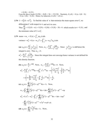
2.69 y[n] + 0.1y[n −1] − 0.06y[n − 2]= 2n
µ[n] with y[–1] = 1 and y[–2] = 0. The complementary
solution yc[n] is obtained by solving yc[n] + 0.1yc[n −1] − 0.06yc[n − 2] = 0. To this end we
set yc[n] = λn
, which yields λn
+ 0.1λn−1
– 0.06λn−2
= λn−2
(λ2
+ 0.1λ – 0.06) = 0 whose
solution gives λ1 = –0.3 and λ2 = 0.2. Thus, the complementary solution is of the form
yc[n] = α1(−0.3)n
+ α2(0.2)n
.
For the particular solution we choose yp[n]= β(2)n
. ubstituting this solution in the difference
equation representation of the system we get β2n
+ β(0.1)2n−1
– β(0.06)2n−2
= 2n
µ[n]. For
n = 0 we get β+ β(0.1)2−1
– β(0.06)2−2
=1 or β = 200 / 207 = 0.9662 .
The total solution is therefore given by y[n] = yc[n] + yp[n] = α1(−0.3)n
+ α2(0.2)n
+
200
207
2n
.
From the above y[−1] = α1(−0.3)−1
+ α2 (0.2)−1
+
200
207
2−1
= 1 and
y[−2] = α1(−0.3)−2
+ α2 (0.2)−2
+
200
207
2−2
= 0 or equivalently, –
10
3
α1 + 5α2 =
107
207
and
100
9
α1 + 25α2 = –
50
207
whose solution yields α1 = –0.1017 and α2 = 0.0356. Hence, the total
solution is given by y[n] = −0.1017(−0.3)n
+ 0.0356(0.2)n
+ 0.9662(2)n
, for n ≥ 0.
2.70 y[n] + 0.1y[n −1] − 0.06y[n − 2]= x[n] − 2x[n − 1] with x[n]= 2n
µ[n], and y[–1] = 1 and y[–2]
= 0. For the given input, the difference equation reduces to
y[n] + 0.1y[n −1] − 0.06y[n − 2]= 2n
µ[n] − 2(2n −1
)µ[n −1] = δ[n]. The solution of this
28

32. equation is thus the complementary solution with the constants determined from the given
initial conditions y[–1] = 1 and y[–2] = 0.
From the solution of the previous problem we observe that the complementary is of the
form yc[n] = α1(−0.3)n
+ α2(0.2)n
.
For the given initial conditions we thus have
y[−1] = α1(−0.3)−1
+ α2 (0.2)−1
= 1 and y[−2] = α1(−0.3)−2
+ α2 (0.2)−2
= 0. Combining these
two equations we get
−1 / 0.3 1/ 0.2
1/ 0.09 1 / 0.04






α1
α2





 =
1
0





 which yields α1 = − 0.18 and α2 = 0.08.
Therefore, y[n] = − 0.18(−0.3)n
+ 0.08(0.2)n
.
2.71 The impulse response is given by the solution of the difference equation
y[n] + 0.5y[n − 1]= δ[n]. From the solution of Problem 2.68, the complementary solution is
given by yc[n] = α(−0.5)n
. To determine the constant we note y[0] = 1 as y[–1] = 0. From
the complementary solution y[0] = α(–0.5)0
= α, hence α = 1. Therefore, the impulse
response is given by h[n]= (−0.5)n
.
2.72 The impulse response is given by the solution of the difference equation
y[n] + 0.1y[n −1] − 0.06y[n − 2]= δ[n]. From the solution of Problem 2.69, the complementary
solution is given by yc[n] = α1(−0.3)n
+ α2(0.2)n
. To determine the constants α1 and α2 , we
observe y[0] = 1 and y[1] + 0.1y[0] = 0 as y[–1] = y[–2] = 0. From the complementary
solution y[0] = α1(−0.3)0
+ α2(0.2)0
= α1 + α2 = 1, and
y[1] = α1(−0.3)1
+ α2 (0.2)1
= –0.3α1 + 0.2α2 = −0.1. Solution of these equations yield α1 = 0.6
and α2 = 0.4. Therefore, the impulse response is given by h[n]= 0.6(−0.3)n
+ 0.4(0.2)n
.
2.73 Let An = nK
(λi )n
. Then
An+1
An
=
n +1
n
K
λi . Now lim
n→∞
n + 1
n
K
= 1. Since λi < 1, there exists
a positive integer No such that for all n > No , 0 <
An +1
An
<
1 + λi
2
< 1. Hence Ann =0
∞
∑
converges.
2.74 (a) x[n]= 3 −2 0 1 4 5 2{ }, −3 ≤ n ≤ 3. rxx[l ] = x[n]x[n − l ]n =−3
3
∑ . Note,
rxx[−6] = x[3]x[−3]= 2 × 3 = 6, rxx[−5]= x[3]x[−2]+ x[2]x[−3] = 2 × (−2) + 5 × 3 =11,
rxx[−4] = x[3]x[−1] + x[2]x[−2] + x[1]x[−3] = 2 × 0 + 5 × (−2) + 4 × 3 = 2,
rxx[−3]= x[3]x[0]+ x[2]x[−1] + x[1]x[−2] + x[0]x[−3] = 2 ×1 + 5 × 0 + 4 × (−2) +1× 3= −3,
rxx[−2] = x[3]x[1] + x[2]x[0]+ x[1]x[−1]+ x[0]x[−2] + x[−1]x[−3] =11,
rxx[−1] = x[3]x[2] + x[2]x[1]+ x[1]x[0] + x[0]x[−1] + x[−1]x[−2] + x[−2]x[−3]= 28,
rxx[0] = x[3]x[3] + x[2]x[2]+ x[1]x[1] + x[0]x[0] + x[−1]x[−1] + x[−2]x[−2] + x[−3]x[−3] = 59.
The samples of rxx[l ] for 1≤ l ≤ 6 are determined using the property rxx[l ] = rxx[−l ]. Thus,
rxx[l ] = 6 11 2 −3 11 28 59 28 11 −3 2 11 6{ }, −6 ≤ l ≤ 6.
y[n] = 0 7 1 −3 4 9 −2{ }, −3 ≤ n ≤ 3. Following the procedure outlined above we get
29

33. ryy[l ] = 0 −14 61 43 −52 10 160 10 −52 43 61 −14 0{ }, −6 ≤ l ≤ 6.
w[n]= −5 4 3 6 −5 0 1{ }, −3 ≤ n ≤ 3. Thus,
rww[l ] = −5 4 28 −44 −11 −20 112 −20 −11 −44 28 4 −5{ }, −6 ≤ l ≤ 6.
(b) rxy[l ] = x[n]y[n − l ]n =−3
3
∑ . Note, rxy[−6] = x[3]y[−3]= 0,
rxy[−5]= x[3]y[−2]+ x[2]y[−3] =14, rxy[−4] = x[3]y[−1] + x[2]y[−2] + x[1]y[−3] = 37,
rxy[−3]= x[3]y[0]+ x[2]y[−1] + x[1]y[−2] + x[0]y[−3] = 27,
rxy[−2] = x[3]y[1] + x[2]y[0]+ x[1]y[−1]+ x[0]y[−2] + x[−1]y[−3]= 4,
rxy[−1] = x[3]y[2] + x[2]y[1]+ x[1]y[0] + x[0]y[−1] + x[−1]y[−2] + x[−2]y[−3]= 27,
rxy[0] = x[3]y[3] + x[2]y[2]+ x[1]y[1] + x[0]y[0]+ x[−1]y[−1] + x[−2]y[−2]+ x[−3]y[−3]= 40,
rxy[1] = x[2]y[3]+ x[1]y[2] + x[0]y[1] + x[−1]y[0] + x[−2]y[−1] + x[−3]y[−2] = 49,
rxy[2] = x[1]y[3]+ x[0]y[2] + x[−1]y[1] + x[−2]y[0] + x[−3]y[−1]= 10,
rxy[3] = x[0]y[3] + x[−1]y[2]+ x[−2]y[1]+ x[−3]y[0] = −19,
rxy[4] = x[−1]y[3] + x[−2]y[2]+ x[−3]y[1] = −6, rxy[5]= x[−2]y[3]+ x[−3]y[2]= 31,
rxy[6]= x[−3]y[3] = −6. Hence,
rxy[l ] = 0 14 37 27 4 27 40 49 10 −19 −6 31 −6,{ }, −6 ≤ l ≤ 6.
rxw[l ] = x[n]w[n − l ]n =−3
3
∑ = −10 −17 6 38 36 12 −35 6 1 29 −15 −2 3{ },
−6 ≤ l ≤ 6.
2.75 (a) x1[n] = αn
µ[n]. rxx[l ] = x1[n]x1[n − l ]n =−∞
∞
∑ = αn
n=−∞
∞
∑ µ[n]⋅ αn −l
µ[n − l ]
= α2 n−l
µ[n − l ]n=0
∞
∑ =
α2n−l
n=0
∞
∑ =
α−l
1− α2
, for l < 0,
α2 n−l
n=l
∞
∑ =
αl
1− α2
for l ≥ 0.







Note for l ≥ 0, rxx[l ] =
αl
1 − α2 , and for l < 0, rxx[l ] =
α−l
1 − α2 . Replacing l with −l in the
second expression we get rxx[−l ]=
α−(−l )
1− α2 =
αl
1− α2 = rxx[l ]. Hence, rxx[l ] is an even function
of l .
Maximum value of rxx[l ] occurs at l = 0 since αl
is a decaying function for increasing l
when α < 1.
(b) x2 [n]=
1, 0 ≤ n ≤ N −1,
0, otherwise.



rxx[l ] = x2[n − l ]n =0
N −1
∑ , where x2 [n − l] =
1, l ≤ n ≤ N −1 + l ,
0, otherwise.



30

34. Therefore, rxx[l ] =
0, for l < −(N − 1),
N + l , for – (N –1) ≤ l < 0,
N, forl = 0,
N − l , for 0 < l ≤ N − 1,
0, forl > N −1.








It follows from the above rxx[l ] is a trinagular function of l , and hence is even with a
maximum value of N at l = 0
2.76 (a) x1[n] = cos
πn
M





 where M is a positive integer. Period of x1[n] is 2M, hence
rxx[l ] =
1
2M
x1[n]n=0
2M−1
∑ x1[n + l ] =
1
2M
cos
πn
M





n=0
2M−1
∑ cos
π(n + l )
M






=
1
2M
cos
πn
M





n =0
2M−1
∑ cos
πn
M





 cos
πl
M





 − sin
πn
M





 sin
πl
M












=
1
2M
cos
πl
M





 cos2 πn
M





n=0
2M−1
∑ .
From the solution of Problem 2.16 cos2 πn
M





n =0
2M−1
∑ =
2M
2
= M. Therefore,
rxx[l ] =
1
2
cos
πn
M





 .
(b) x2 [n]= nmodulo 6 = 0 1 2 3 4 5{ }, 0 ≤ n ≤ 5. It is a peridic sequence with a period
6. Thus,, rxx[l ] =
1
6
x2[n]x2[n + l ]n =0
5
∑ , 0 ≤ l ≤ 5. It is also a peridic sequence with a period 6.
rxx[0] =
1
6
(x2[0]x2[0]+ x2[1]x2[1]+ x2[2]x2[2]+ x2[3]x2[3]+ x2[4]x2[4]+ x2[5]x2[5]) =
55
6
,
rxx[1] =
1
6
(x2[0]x2[1] + x2 [1]x2[2]+ x2[2]x2[3] + x2[3]x2[4] + x2 [4]x2[5] + x2 [5]x2[0]) =
40
6
,
rxx[2] =
1
6
(x2[0]x2[2]+ x2[1]x2 [3]+ x2[2]x2[4] + x2 [3]x2[5] + x2[4]x2[0]+ x2[5]x2[1]) =
32
6
,
rxx[3] =
1
6
(x2[0]x2 [3] + x2[1]x2[4] + x2 [2]x2[5] + x2 [3]x2[0]+ x2[4]x2 [1] + x2[5]x2 [2]) =
28
6
,
rxx[4] =
1
6
(x2[0]x2[4] + x2 [1]x2[5] + x2 [2]x2[0]+ x2[3]x2 [1] + x2[4]x2[2]+ x2[5]x2[3]) =
31
6
,
rxx[5]=
1
6
(x2[0]x2[5]+ x2[1]x2[0] + x2[2]x2[1] + x2[3]x2[2]+ x2[4]x2[3] + x2[5]x2[4]) =
40
6
.
(c) x3[n] = (−1)n
. It is a periodic squence with a period 2. Hence,
rxx[l ] =
1
2
x3[n]x3[n + l ]n =0
1
∑ , 0 ≤ l ≤ 1. rxx[0] =
1
2
(x2[0]x2[0] + x2 [1]x2[1]) = 1, and
rxx[1] =
1
2
(x2[0]x2 [1] + x2[1]x2[0]) = −1. It is also a periodic squence with a period 2.
2.77 E{X + Y} = (x + y)pXY(x,y)dxdy∫∫ = xpXY (x,y)dxdy∫∫ + ypXYy (x,y)dxdy∫∫
= x pXY(x,y)dy∫( )∫ dx + y pXY(x,y)dx∫( )∫ dy = xpX (x)dx + y pY(y)dy∫∫
31

35. = E{X} + E{Y}.
From the above result, E{2X} = E(X + X} = 2 E{X}. Similarly, E{cX} = E{(c–1)X + X}
= E{(c–1)X} + E{X}. Hence, by induction, E{cX} = cE{x}.
2.78 C = E (X − κ)2
{ }. To find the value of κ that minimize the mean square error C, we
differentiate C with respect to κ and set it to zero.
Thus
dC
dκ
= E{2(X − κ)} = E{2X} − E{2K} = 2 E{X} − 2K = 0. which results in κ = E{X}, and
the minimum value of C is σx
2
.
2.79 mean = mx = E{x} = xpX(x)dx
−∞
∞
∫
variance = σx
2
= E{(x − mx)2
} = (x− mx)2
pX (x)dx
−∞
∞
∫
(a) pX(x) =
α
π
1
x
2
+ α
2





 . Now, mx =
α
π
xdx
x
2
+ α
2−∞
∞
∫ . Since
x
x
2
+ α
2 is odd hence the
integral is zero. Thus mx = 0 .
σx
2
=
α
π
x
2
dx
x
2
+ α
2−∞
∞
∫ . Since this integral does not converge hence variance is not defined for
this density function.
(b) px(x) =
α
2
e
−α x
. Now, mx =
α
2
x
−∞
∞
∫ e
−α x
dx = 0. Next,
σx
2
=
α
2
x
2
e
−α x
dx
−∞
∞
∫ = α x
2
e
−αx
dx
0
∞
∫ = α
x
2
e
−αx
−α
0
∞
+
2x
α
e
−αx
dx
0
∞
∫










= α 0+
2x
α
e
−αx
−α
0
∞
+
2
α
2 e
−αx
dx
0
∞
∫










=
2
α
2 .
(c) px(x) =
n
l






l =0
n
∑ p
l
1− p( )n−l
δ(x− l ). Now,
mx = x
−∞
∞
∫
n
l






l =0
n
∑ pl 1− p( )
n−l
δ(x−l )dx=
n
l






l =0
n
∑ pl 1− p( )
n −l
=np
σx
2
= E{x
2
} − mx
2
= x
2
−∞
∞
∫
n
l






l =0
n
∑ p
l
1− p( )n−l
δ(x − l )dx − (np)
2
= l 2 n
l






l =0
n
∑ pl 1− p( )
n−l
−n2p2 =n p(1−p).
(d) px(x) =
e
−α
α
l
l!
l =0
∞
∑ δ(x − l) . Now,
32

36. mx = x
−∞
∞
∫
e−α
αl
l!
l =0
∞
∑ δ(x−l )dx = l
l =0
∞
∑
e−ααl
l!
= α.
σx
2
= E{x
2
} − mx
2
=
α
2
x
2 e
−α
α
l
l!
l =0
∞
∑ δ(x − l)
−∞
∞
∫ dx − α
2
= l 2 e−α
αl
l!
l =0
∞
∑ − α2 = α .
(e) px(x) =
x
α
2 e
−x2 / 2α2
µ(x). Now,
mx =
1
α
2 x
2
−∞
∞
∫ e
−x2 /2α2
µ(x)dx =
1
α
2 x
2
0
∞
∫ e
−x2 / 2α2
dx = α π / 2 .
σx
2
= E{x
2
} − mx
2
=
1
α
2 x
3
e
−x2 / 2α2
µ(x)
−∞
∞
∫ dx −
α
2
π
2
= 2 −
π
2





 α
2
.
2.80 Recall that random variables x and y are linearly independent if and only if
E a1x + a2y
2





>0 ∀ a1,a2 except when a1 = a2 = 0, Now,
E a1
2
x
2





+E a2
2
y
2





+E (a1)*a2xy*{ }+E a1(a2 )*x*y{ } = a1
2
E x
2
{ }+ a2
2
E y
2
{ } > 0
∀ a1 and a2 except when a1 = a2 = 0.
Hence if x,y are statistically independent they are also linearly independent.
2.81 σx
2
= E (x − mx)
2
{ } = E x
2
+ mx
2
− 2xmx{ }= E{x
2
} + E{mx
2
} − 2E{xmx}.
Since mx is a constant, hence E{mx
2
} = mx
2
and E{xmx} = mxE{x} = mx
2
. Thus,
σx
2
= E{x
2
} + mx
2
− 2mx
2
= E{x
2
} − mx
2
.
2.82 V = aX + bY. Therefore, E{V} = a E{X} + b E{Y} = a mx + bmy. and
σv
2
= E{(V − mv )
2
} = E{(a(X − mx) + b(Y − my ))
2
}.
Since X,Y are statistically independent hence σv
2
= a
2
σx
2
+ b
2
σy
2
.
2.83 v[n] = ax[n] + by[n]. Thus φvv[n] = E{v[m + n}v[m]}
= E a2
x[m + n}x[m]+ b2
y[m + n}y[m] + abx[m + n]y[m] + abx[m]y[m + n]{ }. Since x[n] and
y[n] are independent,
φvv[n] = E a2
x[m + n}x[m]{ }+ E b2
y[m + n}y[m]{ }= a2
φxx[n] + b2
φyy[n].
φvx[n] = E{v[m + n]x[m]} = E a x[m + n]x[m]+ by[m + n]x[m]{ } = a E x[m + n]x[m]{ }= a φxx[n].
Likewise, φvy[n] = b φyy[n].
2.84 φxy[l]=E x[n + l ]y*[n]{ }, φxy[–l]=E x[n – l ]y*[n]{ }, φyx[l]=E y[n + l ]x*[n]{ }.
Therefore, φyx *[l ]=E y*[n + l ]x[n]{ } =E x[n –l ]y*[n]{ }=φxy[–l].
33

37. Hence φxy[−l ] = φyx*[l l].
Since γ xy[l ] = φxy[l ]−mx(my )*. Thus, γ xy[l ] = φxy[l ] − mx(my )*. Hence,
γ xy[l ] = φxy[l ] − mx(my )*. As a result, γ xy*[l ] = φxy *[l ] − (mx )*my.
Hence, γ xy[−l ] = γyx*[l ].
The remaining two properties can be proved in a similar way by letting x = y.
2.85 E x[n]− x[n − l]
2
{ }≥ 0.
E x[n]
2
{ } + E x[n − l ]
2
{ }− E x[n]x*[n − l ]{ } − E x*[n]x[n − l ]{ } ≥ 0
2φxx[0] − 2φxx[l ] ≥ 0
φxx[0] ≥ φxx[l]
Using Cauchy's inequality E x
2
{ }E y
2
{ }≤ E
2
xy{ }. Hence, φxx[0]φyy[0] ≤ φxy[l ]
2
.
One can show similarly γ xx[0] γyy[0] ≤ γ xy[l ]
2
.
2.86 Since there are no periodicities in {x[n]} hence x[n], x[n+l ] become uncorrelated as l → ∞..
Thus lim
l →∞
γxx[l ] = lim
l →∞
φxx[l ]− mx
2
→ 0. Hence lim
l →∞
φxx[l ] = mx
2
.
2.87 φXX[l ] =
9 + 11l 2
+14 l 4
1+ 3l 2
+ 2l 4 . Now, mX[n]
2
= lim
l →∞
φXX[l ] = lim
l →∞
9 +11l 2
+14l 4
1+ 3l 2
+ 2l 4 = 7.
Hence, mX[n] = m 7. E X[n]
2
( )= φXX[0] = 9. Therefore, σX
2
= φXX[0] − mX
2
= 9 − 7 = 2.
M2.1 L = input('Desired length = '); n = 1:L;
FT = input('Sampling frequency = ');T = 1/FT;
imp = [1 zeros(1,L-1)];step = ones(1,L);
ramp = (n-1).*step;
subplot(3,1,1);
stem(n-1,imp);
xlabel(['Time in ',num2str(T), ' sec']);ylabel('Amplitude');
subplot(3,1,2);
stem(n-1,step);
xlabel(['Time in ',num2str(T), ' sec']);ylabel('Amplitude');
subplot(3,1,3);
stem(n-1,ramp);
xlabel(['Time in ',num2str(T), ' sec']);ylabel('Amplitude');
M2.2 % Get user inputs
A = input('The peak value =');
L = input('Length of sequence =');
N = input('The period of sequence =');
FT = input('The desired sampling frequency =');
DC = input('The square wave duty cycle = ');
% Create signals
T = 1/FT;
34

38. t = 0:L-1;
x = A*sawtooth(2*pi*t/N);
y = A*square(2*pi*(t/N),DC);
% Plot
subplot(211)
stem(t,x);
ylabel('Amplitude');
xlabel(['Time in ',num2str(T),'sec']);
subplot(212)
stem(t,y);
ylabel('Amplitude');
xlabel(['Time in ',num2str(T),'sec']);
0 20 40 60 80 100
-10
-5
0
5
10
Time in 5e-05 sec
0 20 40 60 80 100
-10
-5
0
5
10
Time in 5e-05 sec
M2.3 (a) The input data entered during the execution of Program 2_1 are
Type in real exponent = -1/12
Type in imaginary exponent = pi/6
Type in the gain constant = 1
Type in length of sequence = 41
35

39. 0 10 20 30 40
-1
-0.5
0
0.5
1
Time index n
Real part
0 10 20 30 40
-1
-0.5
0
0.5
1
Time index n
Imaginary part
(b) The input data entered during the execution of Program 2_1 are
Type in real exponent = -0.4
Type in imaginary exponent = pi/5
Type in the gain constant = 2.5
Type in length of sequence = 101
0 10 20 30 40
-0.5
0
0.5
1
1.5
Time index n
Real part
0 10 20 30 40
-0.5
0
0.5
1
1.5
Time index n
Imaginary part
M2.4 (a) L = input('Desired length = ');
A = input('Amplitude = ');
omega = input('Angular frequency = ');
phi = input('Phase = ');
n = 0:L-1;
x = A*cos(omega*n + phi);
stem(n,x);
xlabel('Time index');ylabel('Amplitude');
title(['omega_{o} = ',num2str(omega)]);
(b)
36

40. 0 10 20 30 40 50 60 70 80 90 100
-2
-1
0
1
2
Time index n
ω
o
= 0.14π
0 5 10 15 20 25 30 35 40
-2
-1
0
1
2
Time index n
ω o
= 0.24π
0 10 20 30 40 50 60 70 80 90 100
-2
-1
0
1
2
Time index n
ω
o
= 0.68π
37

41. 0 5 10 15 20 25 30 35 40
-2
-1
0
1
2
Time index n
ω
o
= 0.75π
M2.5 (a) Using Program 2_1 we generate the sequence ˜x1[n] = e− j 0.4πn
shown below
0 5 10 15 20 25 30 35 40
-1
-0.5
0
0.5
1
Time index n
Real part
0 5 10 15 20 25 30 35 40
-1
-0.5
0
0.5
1
Time index n
Imaginary part
(b) Code fragment used to generate ˜x2 [n]= sin(0.6πn + 0.6π) is:
x = sin(0.6*pi*n + 0.6*pi);
38

42. 0 5 10 15 20 25 30 35 40
-2
-1
0
1
2
Time index n
(c) Code fragment used to generate ˜x3[n] = 2cos(1.1πn − 0.5π) + 2sin(0.7πn) is
x = 2*cos(1.1*pi*n - 0.5*pi) + 2*sin(0.7*pi*n);
0 5 10 15 20 25 30 35 40
-4
-2
0
2
4
Time index n
(d) Code fragment used to generate ˜x4[n]= 3sin(1.3πn) − 4cos(0.3πn + 0.45π) is:
x = 3*sin(1.3*pi*n) - 4*cos(0.3*pi*n+0.45*pi);
0 5 10 15 20 25 30 35 40
-6
-4
-2
0
2
4
6
Time index n
(e) Code fragment used to generate
˜x5[n] = 5sin(1.2πn + 0.65π) + 4sin(0.8πn) − cos(0.8πn) is:
x = 5*sin(1.2*pi*n+0.65*pi)+4*sin(0.8*pi*n)-cos(0.8*pi*n);
39

43. 0 5 10 15 20 25 30 35 40
-10
-5
0
5
10
Time index n
(f) Code fragment used to generate ˜x6[n] = n modulo 6 is: x = rem(n,6);
0 5 10 15 20 25 30 35 40
-1
0
1
2
3
4
5
6
Time index n
M2.6 t = 0:0.001:1;
fo = input('Frequency of sinusoid in Hz = ');
FT = input('Samplig frequency in Hz = ');
g1 = cos(2*pi*fo*t);
plot(t,g1,'-')
xlabel('time');ylabel('Amplitude')
hold
n = 0:1:FT;
gs = cos(2*pi*fo*n/FT);
plot(n/FT,gs,'o');hold off
M2.7 t = 0:0.001:0.85;
g1 = cos(6*pi*t);g2 = cos(14*pi*t);g3 = cos(26*pi*t);
plot(t/0.85,g1,'-',t/0.85,g2,'--',t/0.85,g3,':')
xlabel('time');ylabel('Amplitude')
hold
n = 0:1:8;
gs = cos(0.6*pi*n);
plot(n/8.5,gs,'o');hold off
M2.8 As the length of the moving average filter is increased, the output of the filter gets more
smoother. However, the delay between the input and the output sequences also increases
(This can be seen from the plots generated by Program 2_4 for various values of the filter
length.)
40

44. M2.9 alpha = input('Alpha = ');
yo = 1;y1 = 0.5*(yo + (alpha/yo));
while abs(y1 - yo) > 0.00001
y2 = 0.5*(y1 + (alpha/y1));
yo = y1; y1 = y2;
end
disp('Square root of alpha is'); disp(y1)
M2.10 alpha = input('Alpha = ');
yo = 0.3; y = zeros(1,61);
L = length(y)-1;
y(1) = alpha - yo*yo + yo;
n = 2;
while abs(y(n-1) - yo) > 0.00001
y2 = alpha - y(n-1)*y(n-1) + y(n-1);
yo = y(n-1); y(n) = y2;
n = n+1;
end
disp('Square root of alpha is'); disp(y(n-1))
m=0:n-2;
err = y(1:n-1) - sqrt(alpha);
stem(m,err);
axis([0 n-2 min(err) max(err)]);
xlabel('Time index n');
ylabel('Error');
title(['alpha = ',num2str(alpha)])
The displayed output is
Square root of alpha is
0.84000349056114
0 5 10 15 20 25
-0.04
-0.02
0
0.02
0.04
0.06
Time index n
α = 0.7056
M2.11 N = input('Desired impulse response length = ');
p = input('Type in the vector p = ');
d = input('Type in the vector d = ');
[h,t] = impz(p,d,N);
n = 0:N-1;
stem(n,h);
xlabel('Time index n');ylabel('Amplitude');
41

45. 0 10 20 30 40
-1
-0.5
0
0.5
1
1.5
Time index n
M2.12 x = 3 −2 0 1 4 5 2[ ] y = 0 7 1 −3 4 9 −2[ ], w = −5 4 3 6 −5 0 1[ ].
(a) rxx[n] = [6 11 2 -3 11 28 59 28 11 -3 2 11 6],
ryy[n] = [0 -14 61 43 -52 10 160 10 -52 43 61 -14 0],
rww[n] = [–5 4 28 –44 –11 –20 112 –20 –11 –44 28 4 –5].
-6 -4 -2 0 2 4 6
0
10
20
30
40
50
60
Lag index
rxx
[n]
-6 -4 -2 0 2 4 6
-50
0
50
100
150
Lag index
ryy
[n]
-6 -4 -2 0 2 4 6
-50
0
50
100
Lag index
r
ww
[n]
(b) rxy[n] = [ –6 31 –6 –19 10 49 40 27 4 27 37 14 0].
42

46. rxw[n] = [3 –2 –15 29 1 6 –35 12 36 38 6 –17 –10].
-6 -4 -2 0 2 4 6
-50
0
50
100
Lag index
rxy
[n]
-6 -4 -2 0 2 4 6
-50
0
50
Lag index
r
xw
[n]
M2.13 N = input('Length of sequence = ');
n = 0:N-1;
x = exp(-0.8*n);
y = randn(1,N)+x;
n1 = length(x)-1;
r = conv(y,fliplr(y));
k = (-n1):n1;
stem(k,r);
xlabel('Lag index');ylabel('Amplitude');
gtext('r_{yy}[n]');
-30 -20 -10 0 10 20 30
-10
0
10
20
30
Lag index
r
yy
[n]
M2.14 (a) n=0:10000;
phi = 2*pi*rand(1,length(n));
A = 4*rand(1,length(n));
x = A.*cos(0.06*pi*n + phi);
stem(n(1:100),x(1:100));%axis([0 50 -4 4]);
xlabel('Time index n');ylabel('Amplitude');
mean = sum(x)/length(x)
var = sum((x - mean).^2)/length(x)
43

47. 0 20 40 60 80 100
-4
-2
0
2
4
Time index n
0 20 40 60 80 100
-4
-2
0
2
4
Time index n
0 20 40 60 80 100
-4
-2
0
2
4
Time index n
0 20 40 60 80 100
-4
-2
0
2
4
Time index n
mean =
0.00491782302432
var =
2.68081196077671
From Example 2.44, we note that the mean = 0 and variance = 8/3 = 2.66667.
M2.15 n=0:1000;
z = 2*rand(1,length(n));
y = ones(1,length(n));x=z-y;
mean = mean(x)
var = sum((x - mean).^2)/length(x)
mean =
0.00102235365812
var =
0.34210530830959
Using Eqs. (2. 129) and (2.130) we get mX =
1−1
2
= 0, and σX
2
=
(1+ 1)2
22
=
1
3
. It should
be noted that the values of the mean and the variance computed using the above MATLAB
program get closer to the theoretical values if the length is increased. For example, for a length
100001, the values are
mean =
9.122420593670135e-04
44

48. var =
0.33486888516819
45

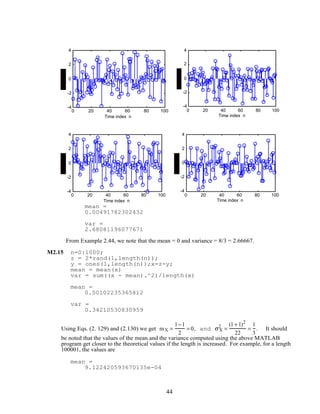
49. Chapter 3 (2e)
3.1 X( e
jω
) = x[n]e−jωn
n =−∞
∞
∑ where x[n] is a real sequence. Therefore,
Xre(ejω
) = Re x[n]e−jωn
n =−∞
∞
∑





 = x[n]Re e−jωn
( )
n =−∞
∞
∑ = x[n]cos(ωn)
n =−∞
∞
∑ , and
Xim (ejω
) = Im x[n]e−jωn
n=−∞
∞
∑





 = x[n]Im e− jωn
( )
n=−∞
∞
∑ = − x[n]sin(ωn)
n=−∞
∞
∑ . Since cos(ωn) and
sin(ωn) are, respectively, even and odd functions of ω , Xre(ejω
) is an even function of ω ,
and Xim (ejω
) is an odd function of ω .
X(ejω
) = Xre
2
(ejω
) + Xim
2
(ejω
) . Now, Xre
2
(ejω
) is the square of an even function and
Xim
2
(ejω
) is the square of an odd function, they are both even functions of ω . Hence,
X(ejω
) is an even function of ω .
arg X(ejω
){ }= tan−1 Xim (ejω
)
Xre (ejω
)





 . The argument is the quotient of an odd function and an even
function, and is therefore an odd function. Hence, arg X(ejω
){ } is an odd function of ω .
3.2 X(e jω
) =
1
1 − α e– jω =
1
1− α e– jω ⋅
1− αe–ω
1− αe–ω =
1− α e–ω
1− 2α cosω + α2 =
1− α cosω − jα sinω
1 − 2αcosω + α2
Therefore, Xre(ejω
) =
1− α cosω
1− 2αcosω + α2 and Xim (ejω
) = –
αsinω
1− 2αcosω + α2 .
X(ejω
)
2
= X(ejω
)⋅ X *(ejω
) =
1
1− αe– jω ⋅
1
1 − α ejω =
1
1− 2α cosω + α2 .
Therefore, X(ejω
) =
1
1− 2α cosω + α2
.
tanθ(ω) =
Xim (ejω
)
Xre (ejω
)
= –
α sinω
1 − α cosω
. Therefore, θ(ω) == tan−1
–
αsinω
1− α cosω





 .
3.3 (a) y[n] = µ[n]= yev[n]+ yod[n], where yev[n]=
1
2
y[n]+ y[−n]( ) =
1
2
µ[n]+ µ[−n]( ) =
1
2
+
1
2
δ[n],
and yod[n]=
1
2
y[n]− y[−n]( ) =
1
2
µ[n]− µ[−n]( ) = µ[n]−
1
2
–
1
2
δ[n].
Now, Yev (ejω
) =
1
2
2π δ(ω + 2πk)
k=–∞
∞
∑







 +
1
2
= π δ(ω+ 2πk) +
1
2
k=–∞
∞
∑ .
Since yod[n]= µ[n]−
1
2
+
1
2
δ[n], yod[n]= µ[n− 1]−
1
2
+
1
2
δ[n −1]. As a result,
45

50. yod[n]− yod[n −1] = µ[n]− µ[n− 1]+
1
2
δ[n −1]−
1
2
δ[n] =
1
2
δ[n]+
1
2
δ[n −1]. Taking the DTFT of
both sides we then get Yod(ejω
) − e−jω
Yod(ejω
) =
1
2
1+ e–jω
( ). or
Yod(ejω
) =
1
2
1+ e−jω
1− e−jω =
1
1− e−jω −
1
2
. Hence,
Y(ejω
) = Yev(ejω
) + Yod(ejω
) =
1
1− e−jω + π δ(ω + 2πk)
k=−∞
∞
∑ .
(b) Let x[n] be the sequence with the DTFT X(ejω
) = 2πδ(ω −ωo + 2πk)
k =−∞
∞
∑ . Its inverse
DTFT is then given by x[n] =
1
2π
2πδ(ω − ωo )ejωn
dω
−π
π
∫ = ejωo
n
.
3.4 Let X(e jω
) = 2π δ(ω + 2πk)k=−∞
∞
∑ . Its inverse DTFT is then given by
x[n]=
1
2π
2π δ(ω)
–π
π
∫ ejωn
dω =
2π
2π
= 1.
3.5 (a) Let y[n] = g[n – no], Then Y(ejω
) = y[n]e−jωn
n=−∞
∞
∑ = g[n− no]e−jωn
n =−∞
∞
∑
= e−jωno g[n]e−jωn
n=−∞
∞
∑ = e−jωn oG(ejω
).
(b) Let h[n] = e jωo
n
g[n], then H(ejω
) = h[n]e−jωn
n=−∞
∞
∑ = ejωo
n
g[n]e−jωn
n =−∞
∞
∑
= g[n]e−j(ω−ωo
)n
n =−∞
∞
∑ = G(ej(ω−ωo
)
).
(c) G(ejω
) = g[n]e−jωn
n=−∞
∞
∑ . Hence
d G(ejω
)( )
dω
= −jng[n]e−jωn
n =−∞
∞
∑ .
Therefore, j
d G(ejω
)( )
dω
= ng[n]e−jωn
n =−∞
∞
∑ . Thus the DTFT of ng[n] is j
d G(ejω
)( )
dω
.
(d) y[n] = g[n] * h[n] = g[k]h[n − k]
k=−∞
∞
∑ . Hence Y(ejω
) = g[k]h[n − k]e−jωn
k=−∞
∞
∑
n=−∞
∞
∑
= g[k]H(ejω
)e−jωk
k =−∞
∞
∑ = H(ejω
) g[k]e−jωk
k=−∞
∞
∑ = H(ejω
)G(ejω
).
(e) y[n] = g[n]h[n]. Hence Y(ejω
) = g[n]h[n]e−jωn
n=−∞
∞
∑
46

51. Since g[n]=
1
2π
G(ejθ
)ejθn
dθ
−π
π
∫ we can rewrite the above DTFT as
Y(ejω
) =
1
2π
h[n]e−jωn
G(ejθ
)ejθn
dθ
−π
π
∫n =−∞
∞
∑ =
1
2π
G(ejθ
) h[n]e−j(ω−θ)n
n=−∞
∞
∑ dθ
−π
π
∫
=
1
2π
G(ejθ
)H(ej(ω−θ)
)dθ
−π
π
∫ .
(f) y[n] = g[n]h*[n]
n =−∞
∞
∑ = g[n]
n=−∞
∞
∑
1
2π
H*(ejω
)e−jωn
dω
−π
π
∫










=
1
2π
H*(ejω
) g[n]
n=−∞
∞
∑ e−jωn







 dω
−π
π
∫ =
1
2π
H*(ejω
)G(ejω
)dω
−π
π
∫ .
3.6 DTFT{x[n]} = X(ejω
) = x[n]e−jωn
n=−∞
∞
∑ .
(a) DTFT{x[–n]} = x[−n]e−jωn
n =−∞
∞
∑ = x[m]ejωm
m=−∞
∞
∑ = X(e−jω
).
(b) DTFT{x*[-n]} = x *[−n]e−jωn
n =−∞
∞
∑ = x[−n]ejωn
n =−∞
∞
∑





 using the result of Part (a).
Therefore DTFT{x*[-n]} = X * (ejω
).
(c) DTFT{Re(x[n])} = DTFT
x[n] + x *[n]
2






=
1
2
X(ejω
) + X * (e− jω
){ } using the result of Part
(b).
(d) DTFT{j Im(x[n])} = DTFT j
x[n] − x *[n]
2j






=
1
2
X(ejω
) − X *(e− jω
){ }.
(e) DTFT xcs[n]{ }= DTFT
x[n]+ x*[−n]
2






=
1
2
X(e jω
) + X *(e jω
){ }= Re X(ejω
){ }= Xre(ejω
).
(f) DTFT xca[n]{ } = DTFT
x[n] − x*[−n]
2






=
1
2
X(ejω
) − X * (e jω
){ }= jXim(e jω
).
3.7 X(ejω
) = x[n]e−jωn
n=−∞
∞
∑ where x[n] is a real sequence. For a real sequence,
X(e jω
) = X *(e– jω
), and IDFT X *(e– jω
),{ }= x *[−n].
47

52. (a) Xre(ejω
) =
1
2
X(ejω
) + X *(e– jω
){ }. Therefore, IDFT Xre(ejω
){ }
=
1
2
IDFT X(ejω
) + X *(e– jω
){ }=
1
2
x[n] + x *[−n]{ } =
1
2
x[n] + x[−n]{ }= xev[n].
(b) jXim (ejω
) =
1
2
X(ejω
) − X * (e– jω
){ }. Therefore, IDFT jXim (ejω
){ }
=
1
2
IDFT X(ejω
) − X *(e– jω
){ }=
1
2
x[n] − x *[−n]{ } =
1
2
x[n] − x[−n]{ }= xod[n].
3.8 (a) X(ejω
) = x[n]e−jωn
n=−∞
∞
∑ . Therefore, X * (ejω
) = x[n]ejωn
n=−∞
∞
∑ = X(e– jω
),and hence,
X * (e– jω
) = x[n]e– jωn
n =−∞
∞
∑ = X(ejω
).
(b) From Part (a), X(e jω
) = X *(e– jω
). Therefore, Xre(ejω
) = Xre(e– jω
).
(c) From Part (a), X(e jω
) = X *(e– jω
). Therefore, Xim (ejω
) = −Xim (e– jω
).
(d) X(ejω
) = Xre
2
(ejω
) + Xim
2
(ejω
) = Xre
2
(e–jω
) + Xim
2
(e–jω
) = X(e−jω
) .
(e) arg X(ejω
) = tan−1 Xim (ejω )
Xre
(e jω )
= −tan−1 Xim (e−jω)
Xre
(e−jω)
= − argX(ejω
)
3.9 x[n] =
1
2π
X(ejω
)ejωn
dω
−π
π
∫ . Hence, x*[n] =
1
2π
X *(ejω
)e–jωn
dω
−π
π
∫ .
(a) Since x[n] is real and even, hence X(ejω
) = X *(ejω
). Thus,
x[– n] =
1
2π
X(ejω
)e−jωn
dω
−π
π
∫ ,
Therefore, x[n] =
1
2
x[n]+ x[−n]( ) =
1
2π
X(ejω
)cos(ωn)dω
−π
π
∫ .
Now x[n] being even, X(ejω
) = X(e– jω
). As a result, the term inside the above integral is even,
and hence x[n] =
1
π
X(ejω
)cos(ωn)dω
0
π
∫
(b) Since x[n] is odd hence x[n] = – x[– n].
Thus x[n] =
1
2
x[n] − x[−n]( ) =
j
2π
X(ejω
)sin(ωn)dω
−π
π
∫ . Again, since x[n] = – x[– n],
48

53. X(ejω
) = −X(e– jω
). The term inside the integral is even, hence x[n] =
j
π
X(ejω
)sin(ωn)dω
0
π
∫
3.10 x[n] = αn
cos(ωo n+ φ)µ[n] = Aαn ejω0
n
ejφ
+ e−jω0
n
e−jφ
2





 µ[n]
=
A
2
ejφ
αe jωo( )
n
µ[n]+
A
2
e−jφ
αe−jωo( )µ[n]. Therefore,
X(ejω
) =
A
2
e jφ 1
1− αe−jωejωo
+
A
2
e−jφ 1
1− αe−jωe−jωo
.
3.11 Let x[n] = αn
µ[n], α <1. From Table 3.1, DTFT{x[n]} = X(e jω
) =
1
1 − α e– jω .
(a) X1(ejω
) = αn
µ[n + 1]e−jωn
n=−∞
∞
∑ = αn
e−jωn
n=−1
∞
∑ = α−1
ejω
+ αn
e−jωn
n =0
∞
∑
= α−1
ejω
+
1
1− αe– jω =
1
α
ejω
− α
1− αe– jω





 .
(b) x2 [n]= nαn
µ[n]. Note that x2 [n]= nx[n]. Hence, using the differentiation-in-frequency
property in Table 3.2, we get X2(e jω
) = j
dX(ejω
)
dω
=
αe−jω
(1− αe−jω
)2 .
(c) x3[n] =
α n
, n ≤ M,
0, otherwise.




Then, X3(e
jω
) = α
n
e
−jωn
+
n=0
M
∑ α
−n
e
−jωn
n=−M
−1
∑
=
1− αM+1
e−jω(M+1)
1− αe−jω + αM
ejωM 1− α−M
e−jωM
1− α−1e−jω .
(d) X4 (ejω
) = αn
n=3
∞
∑ e– jωn
= αn
n =0
∞
∑ e– jωn
−1 − α e− jω
− α2
e− j2ω
=
1
1− αe−jω −1− αe− jω
− α2
e− j2ω
.
(e) X5(ejω
) = nαn
n =−2
∞
∑ e– jωn
= nαn
n=0
∞
∑ e– jωn
− 2α−2
ej2ω
− α−1
e jω
=
αe− jω
(1− αe−jω
)2 − 2α−2
ej2ω
− α−1
e jω
.
(f) X6(ejω
) = αn
n =−∞
−1
∑ e– jωn
= α−m
m=1
∞
∑ e jωm
= α−m
m=0
∞
∑ e jωm
− 1=
1
1− α−1
e jω − 1 =
e jω
α − e jω .
49

54. 3.12 (a) y1[n] =
1, –N ≤ n ≤ N,
0, otherwise.




Then Y1(ejω
) = e−jωn
n=−N
N
∑ = ejωN (1− e−jω(2N+1)
)
(1− e−jω )
=
sin(ω N +
1
2[ ])
sin(ω / 2)
(b) y2
[n] =
1−
n
N
, −N ≤ n ≤ N,
0, otherwise.





Now y2[n] = y0[n] * y0[n] where
y0
[n] =
1, −N / 2 ≤ n ≤ N / 2,
0, otherwise.




Thus Y2 (ejω
) = Y0
2
(ejω
) =
sin2
ω
N +1
2










sin2(ω/ 2)
.
(c) y3[n] =
cos(πn/ 2N), −N ≤ n ≤ N,
0, otherwise.




Then,
Y3(ejω
) =
1
2
e−j(πn / 2N)
e−jωn
n=−N
N
∑ +
1
2
ej(πn / 2N)
e−jωn
n=−N
N
∑
=
1
2
e−j ω−
π
2N



n
n=−N
N
∑ +
1
2
e– j ω+
π
2N



 n
n =−N
N
∑
=
1
2
sin (ω−
π
2N
)(N +
1
2
)( )
sin (ω −
π
2N
)/ 2( )
+
1
2
sin (ω+
π
2N
)(N +
1
2
)( )
sin (ω +
π
2N
)/ 2( )
.
3.13 Denote xm[n] =
(n + m −1)!
n!(m − 1)!
αn
µ[n], α <1. We shall prove by induction that
DTFT xm[n]{ }= Xm(ejω
) =
1
(1− αe– jω
)m . From Table 3.1, it follows that it holds for m = 1.
Let m = 2. Then x2 [n]=
(n + 1)!
n!(
αn
µ[n] = (n + 1)x1[n]= nx1[n]+ x1[n]. Therefore,
X2(e jω
) =
α e– jω
(1− αe– jω
)2 +
1
1− αe– jω =
1
(1− αe– jω
)2 using the differentiation-in-frequency
property of Table 3.2.
Now asuume, the it holds for m. Consider next xm+1[n]=
(n + m)!
n!(m)!
αn
µ[n]
=
n + m
m






(n + m − 1)!
n!(m − 1)!
αn
µ[n],=
n + m
m





 xm[n] =
1
m
⋅ n ⋅xm[n] + xm[n]. Hence,
Xm+1(ejω
) =
1
m
j
d
dω
1
(1− α e– jω
)m








+
1
(1− α e– jω
)m =
α e– jω
(1− αe– jω
)m+1 +
1
(1− α e– jω
)m
=
1
(1− α e– jω
)m+1 .
50

55. 3.14 (a) Xa(ejω
) = δ(ω + 2πk)
k=−∞
∞
∑ . Hence, x[n] =
1
2π
δ(ω)
−π
π
∫ ejωn
dω = 1.
(b) Xb(ejω
) =
1− ejω(N +1)
1− e−jω = e−jωn
n=0
N
∑ . Hence, x[n] =
1, 0 ≤ n ≤ N,
0, otherwise.



(c) Xc(ejω
) =1+ 2 cos(ωl )
l =0
N
∑ = e−jωl
l =−N
N
∑ . Hence x[n] =
1, −N ≤ n ≤ N,
0, otherwise.



(d) Xd(ejω
) =
− jαe−jω
(1− αe−jω )2 , α < 1. Now we can rewrite Xd(ejω
) as
Xd(ejω
) =
d
dω
1
(1− αe−jω)
=
d
dω
Xo(ejω
)( ) where Xo(ejω
) =
1
1− αe−jω .
Now xo[n] = αn
µ[n]. Hence, from Table 3.2, xd [n] = −jnαn
µ[n].
3.15 (a) H1(ejω
) = 1+ 2
ejω
+ e– jω
2





 + 3
ej2ω
+ e– j2ω
2





 = 1+ ejω
+ e– jω
+
3
2
ej2ω
+
3
2
e– j2ω
.
Hence, the inverse of H1(ejω
) is a length-5 sequence given by
h1[n] = 1.5 1 1 1 1.5[ ], − 2 ≤ n ≤ 2.
(b) H2(ejω
) = 3+ 2
ejω
+ e– jω
2





 + 4
ej2ω
+ e– j2ω
2














⋅
ejω /2
+ e– jω/ 2
2





 ⋅ e– jω /2
=
1
2
2ej2ω
+ 3ejω
+ 4 + 4e– jω
+ 3e– j2ω
+ 2e– j3ω
( ). Hence, the inverse of H2(ejω
) is a length-6
sequence given by h2[n]= 1 1.5 2 2 1.5 1[ ], − 2 ≤ n ≤ 3.
(c) H3(ejω
) = j 3 + 4
ejω
+ e– jω
2





 + 2
ej2ω
+ e– j2ω
2














⋅
ejω/2
− e– jω /2
2j






=
1
2
ej3ω
+ 2ej2ω
+ 2ejω
+ 0 − 2e– jω
− 2e– j2ω
− e– j3ω
( ). Hence, the inverse of H3(ejω
) is a
length-7 sequence given by h3[n] = 0.5 1 1 0 –1 –1 − 0.5[ ], − 3≤ n ≤ 3.
(d) H4(e jω
) = j 4 + 2
ejω
+ e– jω
2





 + 3
ej2ω
+ e– j2ω
2














⋅
ejω /2
− e– jω/ 2
2 j





 ⋅ e jω/2
=
1
2
3
2
ej3ω
−
1
2
ej2ω
+ 3ejω
− 3 +
1
2
e– jω
−
3
2
e– j2ω




 . Hence, the inverse of H4(e jω
) is a length-6
sequence given by h4[n]= 0.75 −0.25 1.5 −1.5 0.25 −0.75[ ], − 3≤ n ≤ 2.
3.16 (a) H2(ejω
) =1 + 2cosω +
3
2
(1+ cos2ω) =
3
4
ej2ω
+ ejω
+
5
2
+ e– jω
+
3
4
e– j2ω
.
51

56. Hence, the inverse of H1(ejω
) is a length-5 sequence given by
h1[n] = 0.75 1 2.5 1 0.75[ ], − 2 ≤ n ≤ 2.
(b) H2(ejω
) = 1+ 3cosω +
4
2
(1+ cos2ω)



 cos(ω / 2)ejω/ 2
=
1
2
ej3ω
+
5
4
ej2ω
+
11
4
ejω
+
11
4
+
5
4
e– jω
+
1
2
e– j2ω
. Hence, the inverse of H2(ejω
) is a length-6
sequence given by h2[n]= 0.5 1.25 2.75 2.75 1.25 0.5[ ], − 3 ≤ n ≤ 2.
(c) H3(ejω
) = j 3+ 4cosω + (1+ cos2ω)[ ]sin(ω)
=
1
4
ej3ω
+ ej2ω
+
7
4
ejω
+ 0 −
7
4
e– jω
− e– j2ω
−
1
4
e– j3ω
. Hence, the inverse of H3(ejω
) is a
length-7 sequence given by h3[n] = 0.25 1 1.75 0 −1.75 −1 −0.25[ ], − 3≤ n ≤ 3.
(d) H4(e jω
) = j 4 + 2cosω +
3
2
(1+ cos2ω)



 sin(ω / 2)e– jω/ 2
=
1
2
3
4
ej2ω
+
1
4
e jω
+
9
2
−
9
2
e– jω
+
1
4
e– j2ω
−
3
4
e– j3ω




 . Hence, the inverse of H4(e jω
) is a
length-6 sequence given by h4[n]=
3
8
1
8
9
4
−
9
4
−
1
8
−
3
8



, − 2 ≤ n ≤ 3.
3.17 Y(ejω
) = X(ej3ω
) = X (e jω
)3
( ). Now, X(ejω
) = x[n]e−jωn
n=−∞
∞
∑ . Hence,
Y(ejω
) = y[n]e−jωn
n=−∞
∞
∑ = X (ejω
)3
( )= x[n](e−jωn
)3
= x[m / 3]e−jωm
m=−∞
∞
∑n =−∞
∞
∑ .
Therefore, y[n] =
x[n], n = 0,± 3,± 6,K
0, otherwise.{
3.18 X(ejω
) = x[n]e−jωn
n=−∞
∞
∑ .
X(ejω/ 2
) = x[n]e−j(ω / 2)n
n=−∞
∞
∑ , and X(−ejω / 2
) = x[n](−1)n
e−j(ω / 2)n
n =−∞
∞
∑ . Thus,
Y(ejω
) = y[n]e−ωn
n=−∞
∞
∑ =
1
2
X(ejω / 2
)+ X(−e jω / 2
){ }=
1
2
x[n]+ x[n](−1)n
( )e−j(ω / 2)n
n=−∞
∞
∑ . Thus,
y[n] =
1
2
x[n]+ x[n](−1)n
( )=
x[n], for n even
0. for n odd{ .
3.19 From Table 3.3, we observe that even sequences have real-valued DTFTs and odd sequences
have imaginary-valued DTFTs.
(a) Since −n = n,, x1[n] is an even sequence with a real-valued DTFT.
(b) Since (−n)3
= −n3
, x2[n] is an odd sequence with an imaginary-valued DTFT.
52

57. (c) Since sin(−ωcn) = − sin(ωcn) and ωc(−n) = −ωcn,, x3[n] is an even sequence with a real-
valued DTFT.
(d) Since x4[n] is an odd sequence it has an imaginary-valued DTFT.
(e) Since x5[n] is an odd sequence it has an imaginary-valued DTFT.
3.20 (a) Since Y1(ejω
) is a real-valued function of ω , its inverse is an even sequence.
(b) Since Y2 (ejω
) is an imaginary-valued function of ω , its inverse is an odd sequence.
(c) Since Y3(ejω
) is an imaginary-valued function of ω , its inverse is an odd sequence.
3.21 (a) HLLP(ejω
) is a real-valued function of ω . Hence, its inverse is an even sequence.
(b) HBLDIF(ejω
) is a real-valued function of ω . Hence, its inverse is an even sequence.
3.22 Let u[n] = x[–n], and let X(ejω
) and U(ejω
)denote the DTFTs of x[n] and u[n], respectively.
From the convolution property of the DTFT given in Table 3.2, the DTFT of y[n] = x[n] * u[n]
is given by Y(ejω
) = X(ejω
) U(ejω
). From Table 3.3, U(ejω
) = X(e−jω
). But from Table 3.4,
X(e−jω
) = X *(ejω
). Hence, Y(ejω
) = X(ejω
) X *(ejω
)= X(ejω
)
2
which is real-valued function
of ω .
3.23 From the frequency-shifting property of the DTFT given in Table 3.2, the DTFT of
x[n]e−jπn / 3
is given by X(ej(ω+π /3)
). A sketch of this DTFT is shown below.
ω
0 π/3 2π/3 π
1
–π –2π/3 –π/3
X(ej(ω+π/3)
)
3.24 The DTFT of x[n] = –αn
µ[–n –1] is given by
X(ejω
) = −αn
n=–∞
−1
∑ e– jωn
= − α–n
n=1
∞
∑ ejωn
= −α–1
ejω ejω
α






n=0
∞
∑
n
.
For α > 1, X(ejω
) = −α–1
ejω 1
1− (ejω /α)
=
1
1− α e− jω . X(ejω
)
2
=
1
1+ α2 − 2αcosω
.
From Parseval's relation,
1
2π
X(ejω
)
2
−π
π
∫ dω = x[n]
2
n=−∞
∞
∑ .
53

58. (a) X(ejω
)
2
=
1
5+ 4cosω
. Hence, α = −2. Therefoe, x[n] = −(−2)n
µ[−n −1].
Now, 4 X(ejω
)
2
0
π
∫ dω = 2 X(ejω
)
2
−π
π
∫ dω = 4π x[n]
2
n=−∞
∞
∑ = 4π (−2)n 2
n =−∞
−1
∑
= 4π
1
4






n
n =1
∞
∑ = π
1
4






n
n=0
∞
∑ =
4π
3
.
(b) X(ejω
)
2
=
1
3.25 − 3cosω
. Hence, α =1.5 and therefore, x[n] = −(1.5)n
µ[−n −1]. Now,
X(ejω
)
2
0
π
∫ dω =
1
2
X(ejω
)
2
−π
π
∫ dω = π x[n]
2
n=−∞
∞
∑ = π (1.5)n 2
n=−∞
−1
∑ = π
4
9






n
n=1
∞
∑
=
4π
9
4
9






n
n=0
∞
∑ =
4π
9
⋅
9
5
=
4π
5
.
(c) Using the differentiation-in-frequency property of the DTFT, the inverse DTFT of
X(ejω
) = j
d
dω
1
1− α e−jω





 =
αe−jω
(1− αe−jω )2 is x[n] = −nαn
µ[−n −1]. Hence, the inverse DTFT of
1
(1−α e−jω )2 is −(n +1)αn
µ[−n −1].
Y(ejω
)
2
=
1
(5− 4cosω)2 . Hence, α = 2 and y[n] = −(n +1)2n
µ[−n −1]. Now,
4 X(ejω
)
2
0
π
∫ dω = 2 X(ejω
)
2
−π
π
∫ dω = 4π x[n]
2
n=−∞
∞
∑ = 4π (n +1)2
⋅22n
n =−∞
−1
∑
= π
1
4






n
n=0
∞
∑ ⋅ n2
= π
9 / 4
9/16
= 4π..
3.25 (a) X(ej0
) = x[n]
n=−∞
∞
∑ = 3 +1− 2− 3+ 4+1−1= 3.
(b) X(ejπ
) = x[n]
n=−∞
∞
∑ e jπn
= −3−1− 2 + 3− 4 −1+1= −7.
(c) X(ejω
)
−π
π
∫ dω = 2πx[0]= −4π.
(d) X(ejω
)
2
−π
π
∫ dω = 2π x[n]
2
n=−∞
∞
∑ = 82π. (Using Parseval's relation)
54

59. (e)
dX(ejω
)
dω
2
−π
π
∫ dω = 2π n⋅x[n]
2
n=−∞
∞
∑ = 378π. (Using Parseval's relation with differentiation-in-
frequency property)
3.26 (a) X(ej0
) = x[n]
n=−∞
∞
∑ = −2 + 4− 1+ 5 −3 − 2+ 4+ 3 = 8.
(b) X(ejπ
) = x[n](−1)n
n=−∞
∞
∑ = 2 + 4 +1+ 5+ 3− 2 − 4 +3 = 14.
(c) X(ejω
)
−π
π
∫ dω = 2πx[0]= −4π.
(d) X(ejω
)
2
−π
π
∫ dω = 2π x[n]
2
n=−∞
∞
∑ = 168π. (Using Parseval's relation)
(e)
dX(ejω
)
dω
2
−π
π
∫ dω = 2π n⋅x[n]
2
n=−∞
∞
∑ = 1238π.
3.27 Let G1(e jω
) denote the DTFT of g1[n].
(b) g2[n]= g1[n]+ g1[n− 4]. Hence, the DTFT of g2[n] is given by
G2(ejω
) = G1(ejω
)+ e−j4ω
G1(ejω
) = (1+ e−j4ω
)G1(ejω
).
(c) g3[n] = g1[−(n −3)]+ g1[n − 4]. Now, the DTFT of g1[−n] is given by G1(e−jω
).
Hence, the DTFT of g3[n] is given by G3(e jω
) = e−j3ω
G1(e−jω
)+ e−j4ω
G1(ejω
).
(d) g4[n]= g1[n]+ g1[−(n− 7)]. Hence, the DTFT of g4[n] is given by
G4(ejω
) = G1(ejω
) + e−j7ω
G1(e−jω
).
3.28 Y(ejω
) = X1(ejω
)⋅X2(ejω
)⋅X3(ejω
),i.e.,
y[n]
n =−∞
∞
∑ e−jωn
= x1[n]
n=−∞
∞
∑ e−jωn







 x2[n]
n =−∞
∞
∑ e−jωn







 x3[n]
n =−∞
∞
∑ e−jωn








(a) Therefore, setting ω = 0 we get y[n]
n =−∞
∞
∑ = x1[n]
n =−∞
∞
∑







 x2[n]
n=−∞
∞
∑







 x3[n]
n =−∞
∞
∑







 .
(b) Setting ω = π we get (−1)n
y[n]
n =−∞
∞
∑ = (−1)n
x1[n]
n =−∞
∞
∑







 (−1)n
x2[n]
n=−∞
∞
∑







 (−1)n
x3[n]
n=−∞
∞
∑







 .
55

60. 3.29 (a) x[n] = xev[n]+ xod[n]. Now, for a causal x[n], from the results of Problem 2.4(??), we
observe
x[n] = 2xev[n]µ[n]− x[0]δ[n] = h[n]− x[0]δ[n], (1)
x[n] = 2xod[n]µ[n]+ x[0]δ[n]. (2)
Taking the DTFT of both sides of Eq. (2) we get
X(ejω
) = H(ejω
)− x[0], (3)
where H(ejω
) = DTFT 2xev[n]µ[n]{ }=
1
π
Xre(ejθ
)
–π
π
∫ m(ej(ω−θ)
)dθ, (4)
Note: The DTFT of xev[n] is Xre(ejω
), and the DTFT of µ[n] is m(ejω
).
Now, from Table 3.1, m(ejω
) =
1
1− e−jω + π δ(ω + 2πk)
k =−∞
∞
∑ =
1
2
−
j
2
cot
ω
2





 + π δ(ω + 2πk)
k =−∞
∞
∑ .
Substituting the above in Eq. (4) we get
H(ejω
) =
1
π
Xre(ejθ
)
–π
π
∫
1
2
−
j
2
cot
θ
2





 + π δ(θ+ 2πk)
k=−∞
∞
∑








dθ
= Xre(ejω
)+
1
2π
Xre(ejθ
)
–π
π
∫ dθ−
j
2π
Xre(ejθ
)
–π
π
∫ cot
ω − θ
2





 dθ.
Substituting the above in Eq. (3) we get
X(ejω
) = Xre(e jω
)+ jXim(ejω
) = H(ejω
)− x[0]
= Xre(ejω
)+
1
2π
Xre(ejθ
)
–π
π
∫ dθ−
j
2π
Xre(ejθ
)
–π
π
∫ cot
ω − θ
2





 dθ − x[0]
= Xre(ejω
)−
j
2π
Xre(ejθ
)
– π
π
∫ cot
ω− θ
2





 dθ, (5)
since
1
2π
Xre(ejθ
)
–π
π
∫ dθ= x[0],as x[n] is real. Comparing the imaginary part of both sides of
Eq. (5) we therefore get Xim(ejω
)= –
1
2π
Xre(e jθ
)
–π
π
∫ cot
ω − θ
2





 dθ.
(b) Taking the DTFT of both sides of Eq. (2) we get
X(ejω
) = G(ejω
)+ x[0], (6)
where, G(ejω
) = DTFT 2xod[n]µ[n]{ }=
j
π
Xim (ejθ
)
–π
π
∫ m(ej(ω−θ)
)dθ, (7)
as jXim(ejω
) is the DTFT of xod[n]. Substituting the expression for m(ejω
) given above in
Eq. (7) we get G(ejω
) =
j
π
Xim (ejθ
)
–π
π
∫
1
2
−
j
2
cot
θ
2





 + π δ(θ + 2πk)
k =−∞
∞
∑








dθ
56

61. = jXim(ejω
)+
j
2π
Xim(ejθ
)
–π
π
∫ dθ +
1
2π
Xim(ejθ
)
– π
π
∫ cot
ω − θ
2





 dθ
Substituting the above in Eq. (6) we get
X(ejω
) = Xre(e jω
)+ jXim(ejω
) = G(ejω
)+ x[0]
= jXim(ejω
)+
j
2π
Xim(ejθ
)
–π
π
∫ dθ +
1
2π
Xim(ejθ
)
– π
π
∫ cot
ω − θ
2





 dθ + x[0]
= jXim(ejω
)+
1
2π
Xim (ejθ
)
–π
π
∫ cot
ω − θ
2





 dθ+ x[0] (8)
as
1
2π
Xim (ejθ
)
–π
π
∫ dθ = 0 since Xim(ejω
) is an odd function of ω. Comparing the real parts of
both sides of Eq. (8) we finally arrive at Xre(ejω
)=
1
2π
Xim (ejθ
)
–π
π
∫ cot
ω − θ
2





 dθ + x[0].
3.30 S = WN
−(k −l)n
n =0
N−1
∑ = ej2πn(k −l)/ N
n=0
N−1
∑
If k – l ≠ rN then S =
1− ej2πn(k−l)
1− ej2πn(k −l)/ N =
1− 1
1− ej2πn(k−l) / N = 0.
If k – l = rN then S = WN
−rnN
n=0
N −1
∑ = e−j2πnr
n =0
N −1
∑ = 1
n=0
N−1
∑ = N .
Hence, WN
−(k−l)n
n=0
N −1
∑ =
N, for k – l = rN, r an integer,
0, otherwise.



3.31 ˜y[n] = ˜x[r]˜h[n − r]
r=0
N −1
∑ . Then ˜y[n + kN] = ˜x[r]˜h[n + kN− r]
r=0
N −1
∑ . Since ˜h[n] is periodic in n
with a period N, ˜h[n + kN − r] = ˜h[n − r]. Therefore ˜y[n + kN] = ˜x[r]˜h[n − r]
r=0
N −1
∑ = ˜y[n], hence
˜y[n] is also periodic in n with a period N.
3.32 ˜x[n] = 0 1 0 −2 3{ } and ˜h[n] = 2 0 1 0 −2{ }.
Now, ˜y[0]= ˜x[r]˜h[0 − r]
r=0
4
∑ = ˜x[0]˜h[0]+ ˜x[1] ˜h[4] + ˜x[2]˜h[3]+ ˜x[3]˜h[2]+ ˜x[4]˜h[1] = –4.
Similarly ˜y[1]= ˜x[r]˜h[1− r]
r=0
3
∑ = ˜x[0]˜h[1]+ ˜x[1]˜h[0]+ ˜x[2] ˜h[3]+ ˜x[3] ˜h[2] = 5.
Continuing the process we can show that ˜y[2]= 4, ˜y[3]= −9, and ˜y[4]= 6.
57

62. 3.33 ˜x[n] = 2 −1 2 3 −2{ } and ˜h[n] = 1 2 −3 0 −3{ }.
Now, ˜y[0]= ˜x[r]˜h[0 − r]
r=0
4
∑ = ˜x[0]˜h[0]+ ˜x[1] ˜h[4] + ˜x[2]˜h[3]+ ˜x[3]˜h[2]+ ˜x[4]˜h[1] = –8.
Similarly ˜y[1]= ˜x[r]˜h[1− r]
r=0
3
∑ = ˜x[0]˜h[1]+ ˜x[1]˜h[0]+ ˜x[2] ˜h[3]+ ˜x[3] ˜h[2] = 3.
Continuing the process we can show that ˜y[2]= −15, ˜y[3]= 16, and ˜y[4]= −8.
3.34 Since ˜ψ k[n + rN] = ˜ψ k[n], hence all the terms which are not in the range 0,1,....N-1 can be
accumulated to ˜ψ k[n], where 0 ≤ k ≤ N –1. Hence in this case the Fourier series representation
involves only N complex exponential sequences. Let
˜x[n] =
1
N
˜X[k]ej2πkn/ N
k =0
N−1
∑ then
˜x[n]
n=0
N −1
∑ e−j2πrn / N
=
1
N
˜X[k]e j2π(k −r)n / N
k =0
N−1
∑
n=0
N −1
∑ =
1
N
˜X[k] ej2π(k −r)n / N
n =0
N −1
∑
k =0
N−1
∑ .
Now from Eq. (3.28), the inner summation is equal to N if k = r, otherwise it is equal to 0.
Thus ˜x[n]
n=0
N −1
∑ e−j2πrn / N
= ˜X[r].
˜X[k + l N]= ˜x[n]
n =0
N−1
∑ e−j2π(k+l N)n / N
= ˜x[n]
n =0
N−1
∑ e−j2πkn / N
e−j2πl n
= ˜x[n]
n=0
N−1
∑ e−j2πkn/ N
= ˜X[k].
3.35 (a) ˜x1[n]= cos
πn
4





 =
1
2
ejπn / 4
+ e−jπn / 4
{ }. The period of ˜x1[n] is N = 8.
˜X1[k] =
1
2
ej2πn / 8
n=0
7
∑ e−j2πkn/ 8
+ e−j2πn / 8
n=0
7
∑ e−j2πkn/ 8








=
1
2
e−j2πn(k −1)/ 8
n=0
7
∑ + e−j2πn(k+1)/ 8
n=0
7
∑








. Now, from Eq. (3.28) we observe
e−j2πn(k −1)/8
n =0
7
∑ =
8, for k = 1,
0, otherwise,{ and e−j2πn(k +1)/ 8
n =0
7
∑ =
8, for k = 7,
0, otherwise.{ Hence,
˜X1[k] =
4, k = 1,7,
0, otherwise.{
(b) ˜x2[n] = sin
πn
3





 + 3cos
πn
4





 =
1
2j
ejπn / 3
− e−jπn / 3
{ }+
3
2
ejπn / 4
+ e−jπn / 4
{ }. The period of
sin
πn
3





 is 6 and the period of cos
πn
4





 is 8. Hence, the period of ˜x2[n] is the gcm of
(6,8) and is 24. ˜X2[k]=
1
2j
ej8πn / 24
n=0
23
∑ e−j2πkn / 24
− e−j8πn / 24
n=0
23
∑ e−j2πkn / 24








58

63. +
3
2
ej6πn / 24
n=0
23
∑ e−j2πkn/ 24
+ e−j6πn / 24
n=0
23
∑ e−j2πkn/ 24








=
1
2j
e−j2πn(k−3)/ 24
n=0
23
∑ − e−j2πn(k +3) /24
n =0
23
∑








+
3
2
e−j2πn(k−4)/ 24
n=0
23
∑ + e−j2πn(k +4)/ 24
n =0
23
∑








.
Hence ˜X2[k]=
− j12, k = 3,
j12, k = 21,
36, k = 4,20,
0, otherwise.





3.36 Since ˜p[n] is periodic with period N, then from Eq. (3.168a) 0f Problem 3.34,
˜p[n] =
1
N
˜P[k]e−j2πkn / N
k =0
N−1
∑ where using Eq. (3.168b) we get ˜P[k] = ˜p[n]e−j2πkn / N
n=0
N −1
∑ = 1.
Hence ˜p[n] =
1
N
e−j2πkn / N
k =0
N−1
∑ .
3.37 ˜X[k] = X(ejω
)
ω=2πk /N
= X(ej2πk /N
) = x[n]e−j2πkn/ N
n=−∞
∞
∑ , – ∞ < k < ∞.
(a) ˜X[k + l N]= X(ej2π(k+l N) / N
) = X(ej2πk / N
e j2πl
) = X(ej2πk / N
) = ˜X[k].
(b) ˜x[n] =
1
N
˜X[k]ej2πkn/ N
k =0
N−1
∑ =
1
N
x[l ]e−j2πkl /N
l =−∞
∞
∑





 ej2πkn/ N
k =0
N−1
∑
=
1
N
x[l]ej2πk(n−l )/N
l =−∞
∞
∑
k =0
N−1
∑ . Let l = n + r ⋅ N . Then ˜x[n]=
1
N
x[n + r ⋅N] e− j2πkr
k=0
N −1
∑






r=−∞
∞
∑ .
But e− j2πkr
k=0
N −1
∑ = N. Hence, ˜x[n]= x[n + r ⋅ N].
r=−∞
∞
∑
3.38 (a) ˜G[k]= ˜g[n]e−j2πkn/ N
n=0
N−1
∑ = ˜x[n]˜y[n]e−j2πkn/ N
n=0
N−1
∑ . Now, ˜x[n] =
1
N
˜X[r]e j2πrn / N
r=0
N−1
∑
Therefore, ˜G[k]=
1
N
˜X[r]˜y[n]e−j2π(k−r)n / N
r=0
N−1
∑
n=0
N−1
∑ =
1
N
˜X[r] ˜y[n]e−j2π(k−r)n / N
n=0
N −1
∑
r=0
N−1
∑
=
1
N
˜X[r] ˜Y[k − r]
r=0
N−1
∑ .
(b) ˜h[n] =
1
N
˜X[k] ˜Y[k]ej2πkn/ N
k =0
N−1
∑ =
1
N
˜x[r]
r=0
N−1
∑ ˜Y[k]ej2πk(n−r)/ N
k =0
N−1
∑
59

64. = ˜x[r]
1
N
˜Y[k]ej2πk(n−r)/ N
k =0
N−1
∑








r=0
N −1
∑ = ˜x[r]˜y[n − r]
r=0
N −1
∑ .
3.39 (a) y[n] = αg[n] +βh[n]. Therefore
Y[k]= y[n]WN
nk
n =0
N−1
∑ = α g[n]WN
nk
n=0
N−1
∑ + β h[n]WN
nk
n=0
N −1
∑ = αG[k]+ βH[k]
(b) x[n] = g[< n − n0 >N]. Therefore X[k] = g[< n − n0 >N ]WN
nk
n=0
N −1
∑
= g[N + n − n0]WN
nk
n=0
n 0
−1
∑ + g[n − n0 ]WN
nk
n =n0
N −1
∑
= g[n]WN
(n +n 0 −N)k
n =N −n0
N−1
∑ + g[n]WN
(n+n 0 )k
n=0
N−n0
−1
∑ = WN
n0k
g[n]WN
nk
n=0
N−1
∑ = WN
n0k
G[k].
(c) u[n] = WN
−k0n
g[n]. Hence U[k]= u[n]WN
nk
n =0
N−1
∑ = g[n]WN
(k−k0 )n
n=0
N −1
∑
=
WN
(k−k 0
)n
g[n],
n =0
N−1
∑ if k ≥ k0,
WN
(N +k−k0
)n
g[n],
n=0
N−1
∑ if k < k0
.








Thus, U[k]=
G[k − k0
], if k ≥ k0
,
G[N + k − k0], if k < k0,



= G[< k − k0 >N ].
(d) h[n] = G[n]. Therefore, H[k] = h[n]WN
nk
n=0
N−1
∑ = G[n]WN
nk
n=0
N −1
∑ = g[r]Wnr
Wkr
r=0
N−1
∑
n =0
N −1
∑
= g[r] W
(k+r)n
n=0
N −1
∑
r=0
N −1
∑ .
The second sum is non-zero only if k = r = 0 or else if r = N – k and k ≠ 0. Hence,
H[k] =
Ng[0], if k = 0,
Ng[N − k], if k > 0,
= Ng[< −k >N]



.
(e) u[n] = g[m]h[< n − m >N ]
m=0
N−1
∑ . Therefore, U[k]= g[m]h[< n− m >N ]
m=0
N−1
∑
n =0
N−1
∑ WN
nk
= g[m] h[< n − m >N ]
n =0
N−1
∑
m=0
N −1
∑ WN
nk
= g[m]H[k]
m=0
N−1
∑ WN
mk
= H[k]G[k].
60

65. (f) v[n] = g[n]h[n]. Therefore, V[k]= g[n]h[n]
n =0
N−1
∑ WN
nk
=
1
N
h[n]G[r]Wnk
W−nr
=
r=0
N −1
∑
n=0
N−1
∑
1
N
G[r] h[n]W(k−r)n
n =0
N−1
∑
r=0
N−1
∑ =
1
N
G[r]H[< k − r >N ]
r=0
N−1
∑ .
(g) x[n] =
1
N
X[k]W−nk
k =0
N−1
∑ . Thus x*[n] =
1
N
X *[k]Wnk
k=0
N −1
∑ . Therefore,
x[n]
2
n=0
N −1
∑ =
1
N2 X[r]W−nr
r=0
N−1
∑








n=0
N −1
∑ X*[l ]Wnl
l =0
N−1
∑







 =
1
N2 X[r]X*
[l] Wn(l −r)
n=0
N−1
∑
l =0
N −1
∑
r=0
N−1
∑ .
Since the inner sum is non-zero only if l = r, we get x[n]
2
n=0
N −1
∑ =
1
N
X[k]
2
.
k =0
N−1
∑
3.40 X[k] = x[n]W
nk
n=0
N −1
∑ .
(a) X*[k] = x*[n]W−nk
n=0
N −1
∑ . Replacing k by N – k on both sides we obtain
X*[N – k] = x*[n]W−n(N−k)
n=0
N −1
∑ = x*[n]
n =0
N−1
∑ Wnk
. Thus x*[n] ⇔ X*[N – k] = X*[< –k >N].
(b) X*[k] = x*[n]W−nk
n=0
N −1
∑ . Replacing n by N – n in the summation we get
X*[k] = x*[N − n]W−(N −n)k
n=0
N −1
∑ = x*[N − n]Wnk
n=0
N−1
∑ .
Thus x*[N – n] = x*[< –n >N] ⇔ X*[k].
(c) Re{x[n]} =
1
2
{x[n] + x*[n]}. Now taking DFT of both sides and using results of part (a)
we get Re{x[n]} ⇔
1
2
{X[k] + X*[< –k >N]}.
(d) j Im{x[n]} =
1
2
{x[n] – x*[n]} this imples j Im{x[n]}⇔
1
2
{X[k] – X*[< –k >N]}.
(e) xpcs[n] =
1
2
{x[n] + x*[<–n >N]} Using linearity and results of part (b) we get
xpcs[n] ⇔
1
2
{X[k] + X*[k]} = Re{X[k]}.
(f) xpca[n] =
1
2
{x[n] – x*[< –n >N]}. Again using results of part (b) and linearity we get
xpca[n] ⇔
1
2
{X[k] –X*[k]} = j Im {X[k]}.
61

66. 3.41 X[k] = Re{X[k]} + j Im{X[k]} = x[n]e– j2πkn / N
n=0
N −1
∑ .
(a) xpe[n] =
1
2
x[n]+ x[< −n >N ]{ }. From Table 3.6, x*[< −n >N ] ⇔
DFT
X *[k]. Since x[n] is
real, x[< −n >N ]= x*[< −n >N ] ⇔
DFT
X *[k]. Thus, Xpe[k] =
1
2
X[k]+ X *[k]{ }= Re{X[k]}.
(b) xpo[n]=
1
2
x[n]− x[< −n >N ]{ }. As a result, Xpo[k] =
1
2
X[k]− X*[k]{ } = jIm{X[k]}.
3.42 Since for a real sequence, x[n] = x*[n], taking DFT of both sides we get X[k] =
X*[<– k>N]. This implies, Re{X[k]} + j Im{X[k]} = Re{X[<– k>N} – j Im{X[<– k>N}.
Comparing real and imaginary parts we get
Re{X[k]} = Re{X[<– k>N} and Im{X[k]} = – Im{X[<– k>N}.
Also X[k] = Re{X[k]}( )2
+ Im{X[k]}( )2
= Re{X[< –k >N]}( )2
+ –Im{X[< –k >N]}( )2
= X[< –k >N]
and arg{X[k]}= tan−1 Im{X[k]}
Re{X[k]}





 = tan−1 –Im{X[< −k >N ]}
Re{X[< −k >N ]}







 = − arg{X[< −k >]N}.
3.43 (a) x1[< −n >8] = 1 1 1 0 0 0 1 1[ ]= x1[n]. Thus, x1[n] is a periodic even sequence,
and hence it has a real-valued 8-point DFT.
(b) x2 [< −n >8 ]= 1 −1 −1 0 0 0 0 1[ ].. Thus, x2 [n] is neither a periodic even or a
periodic odd sequence. Hence, its 8-point DFT is a complex sequence.
(c) x3[< −n >8] = 0 −1 −1 0 0 0 1 1[ ] = −x3[n]. Thus, x3[n] is a periodic odd
sequence, and hence it has an imaginary-valued 8-point DFT.
(d) x4[< −n >8 ]= 0 1 1 0 0 0 1 1[ ] = x4[n]. Thus, x4[n] is a periodic even sequence,
and hence it has a real-valued 8-point DFT.
3.44 (a) Now, X[N/2] = x[n]WN
nN / 2
n=0
N −1
∑ = (−1)
n
x[n]
n=0
N −1
∑ . Hence if x[n] = x[N – 1 – n] and N is
even, then (−1)
n
x[n]
n=0
N −1
∑ = 0 or X[N/2] = 0.
(b) X[0] = x[n]
n=0
N −1
∑ so if x[n] = – x[N – 1 – n], then X[0] = 0.
62

67. (c ) X[2l ]= x[n]
n=0
N −1
∑ W2nl
= x[n]
n =0
N
2
−1
∑ W2nl
+ x[n]
n=N / 2
N −1
∑ W2nl
= x[n]
n=0
N
2
−1
∑ W2nl
+ x[n +
N
2
]
n=0
N
2
−1
∑ W2nl
= (x[n]
n=0
N
2
−1
∑ + x[n +
N
2
])W2nl
.
Hence if x[n] = – x[n +
N
2
] = – x[n+M], then X[2l ] = 0, for l = 0, 1, . . . . , M – 1.
3.45 X[2m]= x[n]WN
2 mn
n =0
N−1
∑ = x[n]WN
2mn
n=0
N
2
−1
∑ + x[n]WN
2mn
n=
N
2
N −1
∑
= x[n]WN
2mn
n =0
N
2
−1
∑ + x[n +
N
2
]WN
2m(n+
N
2
)
n =0
N
2
−1
∑ = x[n]WN
2mn
n=0
N
2
−1
∑ + x[n +
N
2
]WN
2mn
n=0
N
2
−1
∑ WN
mN
= x[n]+ x[n +
N
2
]





 WN
2mn
n =0
N
2
−1
∑ = 0, 0 ≤ m ≤
N
2
− 1. This implies x[n]+ x[n +
N
2
] = 0.
3.46 (a) Using the circular time-shifting property of the DFT given in Table 3.5 we observe
DFT x[< n − m1 >N{ }= WN
km1
X[k] and DFT x[< n − m2 >N{ } = WN
km2
X[k]. Hence,
W[k]= DFT x[n]{ }= αWN
km1
X[k] + βWN
km2
X[k] = αWN
km1
+ βWN
km2
( )X[k]. A proof of the
circular time-shifting property is given in Problem 3,39.
(b) g[n] =
1
2
x[n] + (−1)n
x[n]( )=
1
2
x[n]+ WN
−
N
2
n
x[n]








, Using the circular frequency-shifting
property of the DFT given in Table 3.5, we get G[k] = DFT g[n]{ }=
1
2
X[k]+ X[< k −
N
2
>N]






.
(c) Using the circular convolution property of the DFT given in Table 3.5 we get
Y[k] = DFT y[n]{ } = X[k]⋅ X[k]= X2
[k]. A proof of the circular convolution property is given in
Problem 3,39.
3.47 (a) DFT x[n −
N
2
]






= WN
k
N
2 X[k] = −X[k]. Hence,
u[k]= DFT u[n]{ }= DFT x[n] + x[n −
N
2
]






= X[k]− X[k] = 0.
(b) V[k] = DFT v[n]{ } = DFT x[n] − x[n −
N
2
]






= X[k] + X[k] = 2 X[k].
63

68. (c) y[n] = (−1)n
x[n]= WN
N
2
n
x[n]. Hence, Y[k] = DFT y[n]{ } = DFT WN
N
2
n
x[n]








= X[< k −
N
2
>N ]
using the circular frequency-shifting property of the DFT given in Table 3.5.
3.48 (a) From the circular frequency-shifting property of the DFT given in Table 3.5,
IDFT X[< k − m1 >N ]{ } = WN
−m1n
x[n] and IDFT X[< k − m2 >N ]{ }= WN
−m2n
x[n]. Hence,
w[n]= IDFT W[k]{ }= IDFT α X[< k − m1 >N +β X[< k − m2 >N{ }
= α WN
−m1n
x[n]+ βWN
−m2n
x[n]= α WN
−m1n
+ βWN
−m2n
( )x[n].
(b) G[k] =
1
2
X[k]+ (−1)k
X[k]( )=
1
2
X[k] + WN
−
N
2
k
X[k]








. Using the circular time-shifting
property of the DFT given in Table 3.5, we get g[n] = IDFT G[k]{ }=
1
2
x[n] + x[< n −
N
2
>N ]





 .
(c) Using the modulation property of the DFT given in Table 3.5 we get
y[n] = IDFT Y[k]{ }= N ⋅ x[n]⋅ x[n]= N ⋅ x2
[n].
3.49 (a) X[2m]= x[n]WN
2 mn
n =0
N−1
∑ = x[n]WN
2mn
n=0
N
2
−1
∑ + x[n]WN
2mn
n=
N
2
N −1
∑
= x[n]WN
2mn
n =0
N
2
−1
∑ + x[n +
N
2
]WN
2m(n+
N
2
)
n =0
N
2
−1
∑ = x[n]WN
2mn
n=0
N
2
−1
∑ + x[n +
N
2
]WN
2mn
n=0
N
2
−1
∑ WN
mN
= x[n]+ x[n +
N
2
]





 WN
2mn
n =0
N
2
−1
∑ = x[n]− x[n]( )WN
2mn
n=0
N
2
−1
∑ = 0, 0 ≤ m ≤
N
2
−1.
(b) X[4l ]= x[n]WN
4ln
n =0
N−1
∑ = x[n]WN
4ln
n=0
N
4
−1
∑ + x[n]WN
4l n
n=
N
4
N
2
−1
∑ + x[n]WN
4ln
n=
N
2
3N
4
−1
∑ + x[n]WN
4l n
n=
3N
4
N −1
∑
= x[n]WN
4l n
+ x[n +
N
4
]WN
4l (n+
N
4
)
+ x[n +
N
2
]WN
4l (n+
N
2
)
+ x[n +
3N
4
]WN
4l (n +
3N
4
)






n =0
N
4
−1
∑
= x[n]+ x[n +
N
4
]WN
l N
+ x[n +
N
2
]WN
2l N
+ x[n +
3N
4
]WN
3l N





n =0
N
4
−1
∑ WN
4l n
= x[n] − x[n]+ x[n] − x[n]( )
n =0
N
4
−1
∑ WN
4l n
= 0 as WN
lN
= WN
2l N
= WN
3l N
= 1.
64

69. 3.50 (a) X[N − k]= x[n]WN
(N−k)n
n =0
N−1
∑ = x[n]WN
−kn
n=0
N −1
∑ = X *[k].
(b) X[0]= x[n]WN
0
n =0
N−1
∑ = x[n]
n=0
N −1
∑ which is real.
(c) X[
N
2
] = x[n]WN
(N /2)n
n=0
N−1
∑ = (−1)n
x[n]
n=0
N−1
∑ which is real.
3.51 (a) H[k] = DFT h[n]{ } = DFT g[{n − 3 >7 ]{ }= W7
3k
G[k]= e
− j
6πk
7 G[k]
= 1+ j2, e
−j
6π
7 (−2 + j3), e
−j
12π
7 (−1− j2), 0, e
−j
24π
7 (8 + j4), e
−j
30π
7 (−3 + j2), e
−j
36π
7 (2 + j5)










(b) h[n]= IDFT H[k]{ } = IDFT G[< k − 4 >7]{ }= W7
−4n
g[n]= e
j
8πn
7 g[n]
= −3.1, 2.4ej8π/ 7
, 4.5ej16π/ 7
, −6ej24π/ 7
, ej32π/7
, −3ej40π/ 7
, 7ej42π/ 7
[ ].
3.52 Y[k] = y[n]WMN
nk
n=0
MN−1
∑ = x[n]WMN
nk
n=0
N −1
∑ . Thus, Y[kM] = x[n]WN
nk
n=0
N −1
∑ = X[k].
Hence, X[k] = Y[kM].
3.53 Note X[k] is the MN-point DFT of the sequence xe[n] obtained from x[n] by appending it
with M(N-1) zeros. Thus, the length-MN sequence y[n] is given by
y[n] = xe
l =0
M−1
∑ [< n − Nl >MN ], 0 ≤ n ≤ MN − 1. Taking the MN-point DFT of both sides we
get Y[k] = WMN
Nkl
l =0
M−1
∑





 X[k] == WM
kl
l =0
M−1
∑





 X[k].
3.54 (a) X[0]= x[n]
n=0
11
∑ = 13.
(b) X[6]= (−1)n
x[n]
n=0
11
∑ = −13.
(c) X[k]
k=0
11
∑ = 12 ⋅ x[0] = 36.
(d) The inverse DFT of e−j(4πk/ 6)
X[k] is x[< n − 4 >12]. Thus,
e−j(4πk /6)
X[k]
k=0
11
∑ =12 ⋅ x[< 0 − 4>12 ]= 12 ⋅x[8]= −48.
65

70. (e) From Parseval's relation, X[k]
2
k=0
11
∑ = 12 ⋅ x[n]
2
n =0
11
∑ = 1500.
3.55 X[8] = X *[< −8>14] = X *[6] = −2 + j3, X[9] = X *[< −9 >14] = X *[5]= 6 − j3,
X[10] = X *[< −10 >14 ]= X *[4]= −2 − j2, X[11] = X *[< −11 >14]= X *[3] =1+ j5,
X[12] = X *[< −12 >14 ]= X *[2] = 3 − j4, X[13]= X *[< −13 >14 ]= X *[1]= −1− j3.
(a) x[0] =
1
14
X[k]
k =0
13
∑ =
32
14
= 2.2857,
(b) x[7] =
1
14
(−1)k
X[k]
k=0
13
∑ = −
12
14
= −0.8571,
(c) x[n]
n =0
13
∑ = X[0] = 12,
(d) Let g[n] = ej(4πn / 7)
x[n]= W14
−4n
x[n]. Then DFT{g[n]} = DFT{W14
−4n
x[n]}= X[< k − 4 >14]
= X[10] X[11] X[12] X[13] X[0] X[1] X[2] X[3] X[4] X[5] X[6] X[7] X[8] X[9][ ]
Thus, g[n]
n =0
13
∑ = ej(4πn/ 7)
x[n]
n=0
13
∑ = X[10] = −2 – j2,
(e) Using Parseval's relation, x[n]
2
n =0
13
∑ =
1
14
X[k]
2
k =0
13
∑ =
498
14
= 35.5714.
3.56 Now yc[n] = g[k]h[< n − k >6 ]
k =0
6
∑ . Hence,
yc[0]= g[0]h[0] + g[1]h[6] + g[2]h[5] + g[3]h[4] + g[4]h[3]+ g[5]h[2]+ g[6]h[1],
yc[1]= g[0]h[1] + g[1]h[0]+ g[2]h[6] + g[3]h[5] + g[4]h[4]+ g[5]h[3] + g[6]h[2],
yc[2]= g[0]h[2] + g[1]h[1]+ g[2]h[0] + g[3]h[6] + g[4]h[5] + g[5]h[4] + g[6]h[3],
yc[3] = g[0]h[3]+ g[1]h[2] + g[2]h[1]+ g[3]h[0] + g[4]h[6]+ g[5]h[5] + g[6]h[4],
yc[4]= g[0]h[4] + g[1]h[3] + g[2]h[2] + g[3]h[1] + g[4]h[0]+ g[5]h[6] + g[6]h[5],
yc[5] = g[0]h[5] + g[1]h[4]+ g[2]h[3] + g[3]h[2] + g[4]h[1]+ g[5]h[0] + g[6]h[6],
yc[6] = g[0]h[6]+ g[1]h[5]+ g[2]h[4] + g[3]h[3] + g[4]h[2] + g[5]h[1]+ g[6]h[0].
Likewise, yL [n]= g[k]h[n − k]
k =0
6
∑ . Hence,
yL [0]= g[0]h[0],
yL [1] = g[0]h[1]+ g[1]h[0],
yL [2]= g[0]h[2]+ g[1]h[1]+ g[2]h[0],
yL [3] = g[0]h[3]+ g[1]h[2]+ g[2]h[1]+ g[3]h[0],
yL [4]= g[0]h[4] + g[1]h[3] + g[2]h[2]+ g[3]h[1] + g[4]h[0],
yL [5] = g[0]h[5] + g[1]h[4]+ g[2]h[3] + g[3]h[2] + g[4]h[1] + g[5]h[0],
yL [6] = g[0]h[6]+ g[1]h[5]+ g[2]h[4] + g[3]h[3] + g[4]h[2] + g[5]h[1] + g[6]h[0],
66

71. yL [7] = g[1]h[6]+ g[2]h[5]+ g[3]h[4]+ g[4]h[3] + g[5]h[2] + g[6]h[1],
yL [8]= g[2]h[6] + g[3]h[5] + g[4]h[4] + g[5]h[3] + g[6]h[2],
yL [9] = g[3]h[6]+ g[4]h[5] + g[5]h[4] + g[6]h[3],
yL [10] = g[4]h[6] + g[5]h[5] + g[6]h[4],
yL [11] = g[5]h[6]+ g[6]h[5],
yL [12] = g[6]h[6].
Comparing y10[n] with yL[n] we observe that
yc[0]= yL[0] + yL[7],
yc[1]= yL [1] + yL[8],
yc[2]= yL[2] + yL [9],
yc[3] = yL [3]+ yL[10],
yc[4]= yL [4] + yL[11],
yc[5] = yL[5] + yL[12],
yc[6] = yL[6].
3.57 Since x[n] is a real sequence, its DFT satisfies X[k] = X *[< −k >N ] where N = 11 in this case.
Therefore, X[1]= X *[< −1>11 X *[10]= 3 + j2,
X[3] = X *[< −3>11 X *[8]= −5 + j8,
X[5] = X *[< −5 >11 X *[6]= 9 + j6,
X[7] = X *[< −7 >11 X *[4] = 2 − j5,
X[9] = X *[< −9 >11 X *[2] = −1− j3.
3.58 The N-point DFT X[k] of a length-N real sequence x[n] satisfy X[k]= X *[< −k >N]. Here N
= 11. Hence, the remaining 5 samples are X[1] = X*[< −1>11] = X*[10] = −3.1− j5.2,
X[4] = X*[< −4 >11] = X *[7] = −4.1− j0.2, X[6] = X *[< −6>11]= X *[5]= 6.5− j9,
X[8] = X*[< −8 >11]= X *[3]= 5.3+ j4.1, X[9] = X *[< −9>11] = X*[2] = −3.2+ j2.
3.59 A length-N periodic even sequence x[n] satisfying x[n] = x*[< −n >N ] has a real-valued N-
point DFT X[k]. Here N = 10. Hence, the remaining 4 samples of x[n] are given by
x[6] = x*[< −6>10] = x*[4] = 2.87− j2, x[7] = x*[< −7>10] = x*[3] = −2.1− j4.6,
x[8] = x*[< −8 >10 ]= x*[2]= −3.25− j1.12, and x[9] = x*[< −9>10] = x*[1] = 0.7+ j0.08.
3.60 As x[n] is a real-valued sequence of length 498, its 498-point DFT X[k] satisfy
X[k] = X *[< −k >498] = X *[498− k] (See Table 3.7).
(a) From the specified DFT samples we observe that X[k1]= X *[412] implying
k1 = 498 − 412 = 86, X[k2 ] = X *[309] implying k2 = 498− 309 =189, X[k3 ]= X *[112] implying
k3 = 498 − 112 = 386, X[k4] = X *[11] implying k4 = 498 −11 = 487.
(b) dc value of {x[n]} = X[0] = 2.
(c) x[n]=
1
498
X[k]W498
−kn
k=0
497
∑ =
1
498
(X[0]+ 2Re X[11]⋅ W498
−11n
{ }+ 2Re X[86]⋅ W498
−86 n
{ }
67

72. + 2Re X[112]⋅W498
−112 n
{ }+ 2Re X[189]⋅ W498
−189 n
{ }+ X[249]⋅ W498
− 249 n
)
=
1
249
{− 0.45 + 7cos
11πn
249





 − 3.1sin
11πn
249





 − 2.2cos
86πn
249





 +1.5sin
86πn
249






+ 3cos
112πn
249





 + 0.7sin
112πn
249





 − 4.7cos
189πn
249





 − 1.9sin
189πn
249





}.
(d) x[n]
2
n =0
497
∑ =
1
498
X[k]
2
k=0
497
∑ = 0.2275.
3.61 As x[n] is a real-valued sequence of length 316, its 316-point DFT X[k] satisfy
X[k]= X *[< −k >316 ] = X *[316− k] (See Table 3.7).
(a) From the specified DFT samples we observe that X[17] = X *[k4 ] implying
k4 = 316 −17 = 299, X[k1] = X*[210] if ε = 0, implying k1 = 316− 210 =106, X[k2 ]= X *[179]
if δ = 0 implying k2 = 316 −179 = 137, and X[k3] = X*[110] if γ = 0 implying
k3 = 316− 110 = 206.
(b) Now, X[0] = x[n]
n=0
315
∑ which is a real number as x[n] are real numbers implying α = 0. Since
the length N = 316 is an even number, X[158]= X[N/ 2] = (−1)n
x[n]
n =0
315
∑ is also a real number
implying β = 0. We have already shown in Part (a), δ = ε = γ = 0.
(c) The dc value of {x[n]} is X[0] = 3.
(d) x[n]=
1
316
{X[0] + 2Re X[17]W316
−17n
( )+ 2Re X[106]W316
−106 n
( )+ 2Re X[137]W316
−137 n
( )
+2 Re X[110]W316
−110 n
( )} =
1
316
{3+ 2(1.5)cos
17πn
158





 + 2(−2.3)sin
106πn
158






+ 2(4.2)cos
137πn
158





 +2(1.72)sin
110πn
158





 − 13}
=
1
316
{−10 + 3cos
17πn
158





 − 4.6sin
106πn
158





 + 8.4)cos
137πn
158





 +3.44 sin
110πn
158





}.
(e) x[n]
2
n =0
315
∑ =
1
316
X[k]
2
k=0
315
∑ = 0.6521.
3.62 {x[n]} = −4, 5, 2, −3, 0, −2, 3, 4{ }, 0 ≤ n ≤ 7. Let X[k] denote the 8-point DFT of
x[n]. Consider the 8-point DFT Y[k]= W4
3k
X[k] = W8
6k
X[k]. Using the circular time-shifting
property of the DFT given in Table 3.5 we observe that the IDFT y[n] of Y[k] is given by
y[n] = x[< n− 6 >8]. Therefore, y[0]= x[< −6 >8 ]= x[2] = 2, y[1]= x[<1− 6 >8] = x[3] = −3,
y[2]= x[< 2 − 6>8] = x[4]= 0, y[3]= x[< 3− 6 >8 ]= x[5]= −2, y[4]= x[< 4 − 6 >8] = x[6]= 3,
68

73. y[5] = x[< 5− 6 >8] = x[7]= 4, y[6] = x[< 6− 6 >8 ]= x[0] = −4, y[7] = x[< 7− 6 >8 ]= x[1] = 5. Thus,
{y[n]} = 2, −3, 0, −2, 3, 4, −4, 5{ }, 0 ≤ n ≤ 7.
3.63 {x[n]} = 1, −1, 2, 3, 0, 0{ }, 0 ≤ n ≤ 5. Let X[k] denote the 6-point DFT of x[n].
Consider the 6-point DFT Y[k] = W3
2k
X[k] = W6
4k
X[k]. Using the circular time-shifting
property of the DFT given in Table 3.5 we observe that the IDFT y[n] of Y[k] is given by
y[n] = x[< n − 4>6 ]. Therefore, y[0] = x[< −4 >6] = x[2] = 2, y[1] = x[< −3 >6 ] = x[3] = 3,
y[2] = x[< −2 >6] = x[4]= 0, y[3] = x[< −1>6 ]= x[5] = 0, y[4] = x[< 0 >6] = x[0] = 1,
y[5]= x[< 1>6 ]= x[1] = −1. Thus, {y[n]} = 2 3 0 0 1 −1{ }, 0 ≤ n ≤ 5.
3.64 (a) yL [0] = g[0]h[0]= −6,
yL [1]= g[0]h[1] + g[1]h[0]= 16,
yL [2] = g[0]h[2]+ g[1]h[1] + g[2]h[0]= 0,
yL [3]= g[0]h[3] + g[1]h[2]+ g[2]h[1] = −19,
yL [4]= g[1]h[3] + g[2]h[2]= 2,
yL [5] = g[2]h[3]= 4.
(b) yc[0]= ge[0]h[0]+ ge[1]h[3] + ge[2]h[2] + ge[3]h[1] == g[0]h[0]+ g[1]h[3]+ g[2]h[2]= −4,
yc[1]= ge[0]h[1]+ ge[1]h[0] + ge[2]h[3] + ge[3]h[2] == g[0]h[1] + g[1]h[0]+ g[2]h[3] = 20,
yc[2]= ge[0]h[2]+ ge[1]h[1]+ ge[2]h[0]+ ge[3]h[3] == g[0]h[2]+ g[1]h[1] + g[2]h[0]= 0,
yc[3] = ge[0]h[3] + ge[1]h[2] + ge[2]h[1] + ge[3]h[0]== g[0]h[3] + g[1]h[2]+ g[2]h[1] = −19.
(c)
Ge[0]
Ge[1]
Ge[2]
Ge[3]














=
1 1 1 1
1 −j −1 j
1 −1 1 −1
1 j −1 − j














−3
2
4
0














=
3
−7 − j2
−1
−7 + j2














,
H[0]
H[1]
H[2]
H[3]














=
1 1 1 1
1 − j −1 j
1 −1 1 −1
1 j −1 −j














2
−4
0
1














=
−1
2 + j5
5
2 − j5














.
Yc[0]
Yc[1]
Yc[2]
Yc[3]














= .
Ge[0]⋅H[0]
Ge[1]⋅H[1]
Ge[2]⋅H[2]
Ge[3]⋅H[3]














=
−3
−4 − j39
−5
−4 + j39














. Therefore
yc[0]
yc[1]
yc[2]
yc[3]














=
1
2
1 1 1 1
1 j −1 −j
1 −1 1 −1
1 − j −1 j














⋅
−3
−4 − j39
−5
−4 + j39














=
−4
20
0
−19














.
3.65 We need to show Ng[n] h[n] = Nh[n] g[n].
Let x[n] = Ng[n] h[n] = g[m]h[< n − m >N ]
m=0
N −1
∑
and y[n] = Nh[n] g[n] = h[m]g[< n − m >N ]
m=0
N −1
∑
69

74. = h[m]g[n− m]
m=0
n
∑ + h[m]g[N + n − m]
m=n +1
N−1
∑
= h[n − m]g[m]
m=0
n
∑ + h[N + n− m]g[m]
m=n +1
N−1
∑ = h[< n − m >N ]g[m]
m=0
N −1
∑ = x[n].
Hence circular convolution is commutative.
3.66 (a) Let g[n] = Nx [n]1
x [n]2 = x1[m]x2[< n − m >N]
m=0
N −1
∑ . Thus,
g[n]
n=0
N −1
∑ = x1[m] x2 [< n − m >N ]
n =0
N−1
∑
m=0
N −1
∑ = x1[n]
n=0
N −1
∑





 x1[m]
m=0
N−1
∑





 . Similarly we can show that if
y[n] = N x [n]3g[n] , then y[n]
n=0
N −1
∑ = g[m] x3[< n − m >N ]
n=0
N −1
∑
m=0
N −1
∑ = g[n]
n=0
N −1
∑





 x3[m]
m=0
N−1
∑






= x1[n]
n=0
N −1
∑ x2[m]
m=0
N−1
∑





 x3[m]
m=0
N−1
∑





 .
(b) (−1)n
g[n]
n=0
N −1
∑ = x1[m] x2[< n − m >N ]
n=0
N−1
∑
m=0
N−1
∑ (−1)n
= x1[m]
m=0
N−1
∑





 x2[N + n − m](−1)n
+ x2[n − m](−1)n
n =m
N −1
∑
n =0
m−1
∑





 .
Replacing n by N+n–m in the first sum and by n–m in the second we obtain
(−1)n
g[n]
n=0
N −1
∑ = x1[m]
m=0
N −1
∑





 x2 [n](−1)n −N +m
+ x2 [n](−1)n +m
n =0
N−1
∑
n=0
m−1
∑






= (−1)n
x1[n]
n=0
N −1
∑





 (−1)n
x2[n]
n=0
N −1
∑





 . Similarly we can show that if y[n] = N x [n]3g[n] , then
(−1)n
y[n]
n=0
N −1
∑ = (−1)n
g[n]
n=0
N −1
∑





 (−1)n
x3[n]
n=0
N−1
∑





 = (−1)n
x1[n]
n=0
N −1
∑





 (−1)n
x2[n]
n=0
N −1
∑





 (−1)n
x3[n]
n=0
N−1
∑





 .
3.67 y[n] = cos
2πln
N





 x[n]=
x[n]
2
e−j2πl n / N
+ ej2πln / N
( )=
1
2
x[n]WN
nl
+
1
2
x[n]WN
−nl
.
Hence Y[k] =
1
2
X[< k + l >N ]+
1
2
X[< k − l >N].
3.68 y[n] = x[4n], 0≤ n ≤
N
4
− 1. Therefore, Y[k] = y[n]WN /4
nk
n =0
N
4
−1
∑ = x[4n]WN /4
nk
n=0
N
4
−1
∑ .
70

75. Now, x[4n] =
1
N
X[m]WN
−4mn
m=0
N−1
∑ =
1
N
X[m]WN/ 4
−mn
m=0
N−1
∑ . Hence,
Y[k] =
1
N
X[m]WN/ 4
−mn
WN/ 4
nk
m=0
N −1
∑
n =0
N
4
−1
∑ =
1
N
X[m] WN /4
(k−m)n
n =0
N
4
−1
∑
m=0
N−1
∑ . Since,
WN /4
(k−m)n
n =0
N
4
−1
∑ =
N
4
, m = k, k +
N
4
, k +
2N
4
, k +
3N
4
,k +
4N
4
,
0, elsewhere,




Thus,
Y[k] =
1
4
X[k] + X[k +
N
4
] + X[k +
2N
4
]+ X[k +
3N
4
]( ).
V[k] = −2 + j3, 1+ j5, −4 + j7, 2 + j6, −1− j3, 4 − j 3 + j8, j6[ ]. Hence,
V *[< −k >8] = −2 − j3, − j6, 3− j8, 4 + j, −1+ j3, 2 − j6, −4 − j7, 1− j5[ ]. Therefore,,
X[k] = −2, 0.5− j0.5, −0.5 − j0.5, 3 + j3.5, −1, 3 − j3.5, −0.5 + j0.5, 0.5 + j0.5[ ] and
Y[k] = 3, 5.5 − j0.5, 7.5 + j3.5, 2.5 + j, −3, 2.5 − j, 7.5 − j3.5, 5.5+ j0.5[ ]
3.69 v[n] = x[n] + jy[n]. Hence, X[k] =
1
2
V[k]+ V* < −k >8 ]{ } is the 8-point DFT of x[n], and
Y[k] =
1
2j
V[k]− V*< −k >8 ]{ } is the 8-point DFT of y[n]. Now,
V[k] = −2 + j3, 1+ j5, −4 + j7, 2 + j6, −1− j3, 4 − j, 3 + j8, j6[ ]
V *[< −k >8]= −2 − j3, −j6, 3− j8, 4 + j, −1+ j3, 2 − j6, −4− j7, 1− j5[ ]. Therefiore,
X[k]= −0.2, 0.5− j0.5, −0.5− j0.5, 3+ j3.5, −1, 3− j3.5, −0.5+ j0.5, 0.5 + j0.5[ ]
Y[k]= 3, 5.5 − j0.5, 7.5+ j3.5, 2.5+ j −3, 2.5− j, 7.5− j3.5, 5.5+ j0.5[ ]
3.70 v[n]= ge[n]+ j h[n] = −3+ j2, 2− j4, 4, j[ ]. Therefore,
V[0]
V[1]
V[2]
V[3]










=
1 1 1 1
1 −j −1 j
1 −1 1 −1
1 j −1 −j










−3+ j2
2− j4
4
j










=
3− j
−12
−1+ j5
−2+ j4










, i.e., {V[k]}= 3− j, −12, −1+ j5, −2+ j4[ ].
Thus, {V*[< −k >4 ]}= 3+ j, −2 − j4, −1− j5, −12[ ]
Therefore, Ge[k] =
1
2
V[k]+ V *[< −k >4]{ }= 3, −7− j2, −1, −7+ j2[ ] and
H[k]=
1
2j
V[k]− V *[< −k >4]{ }= −1, 2+ j5, 5, 2 − j5[ ] .
3.71 v[n]= g[n]+ jh[n]= −2 + j, 1+ j2, −3− j3, 4 + j2[ ]. Therefore,
V[0]
V[1]
V[2]
V[3]










=
1 1 1 1
1 −j −1 j
1 −1 1 −1
1 j −1 −j










−2 + j
1+ j2
−3− j3
4 + j2










=
j2
1+ j7
−10 − j6
1+ j










, i.e., {V[k]}= j2, 1+ j7, −10 − j6, 1+ j[ ].
71

76. Thus, {V*[< −k >4 ]}= −j2, 1− j, −10 + j6, 1− j7[ ].
Therefore, Ge[k] =
1
2
V[k]+ V *[< −k >4]{ }= 0, 1+ j3, −10, 1− j3[ ] and
H[k]=
1
2j
V[k]− V *[< −k >4]{ }= 2, 4, −6, 4[ ].
3.72 (a) Let p[n] = IDFT P[k]{ }. Thus,
p[0]
p[1]
p[2]
p[3]










=
1
4
1 1 1 1
1 j −1 − j
1 −1 1 −1
1 −j −1 j










4
1+ j7
2
1− j7










=
1
4
8
−12
4
16










=
2
−3
1
4










. Similarly, let d[n] = IDFT D[k]{ }.
d[0]
d[1]
d[2]
d[3]










=
1
4
1 1 1 1
1 j −1 − j
1 −1 1 −1
1 −j −1 j










4.5
1.5+ j
−5.5
1.5− j










=
1
4
2
8
−4
12










=
0.5
2
−1
2










. Therefore,
X(ejω
) =
2− 3e−jω
+ e−j2ω
+ 4e−j3ω
0.5+ 2e−jω − e−j2ω + 3e−j3ω .
(b) Let p[n] = IDFT P[k]{ }. Thus,
p[0]
p[1]
p[2]
p[3]










=
1
4
1 1 1 1
1 j −1 − j
1 −1 1 −1
1 −j −1 j










7
7+ j2
−9
7− j2










=
3
3
−4
5










. Similarly, let
d[n] = IDFT D[k]{ }. Thus,
d[0]
d[1]
d[2]
d[3]










=
1
4
1 1 1 1
1 j −1 − j
1 −1 1 −1
1 −j −1 j










0
4 + j6
−4
4 − j6










=
1
−2
−3
4










. Therefore,
X(ejω
) =
3+ 3e−jω
− 4e−j2ω
+ 5e−j3ω
1− 2e−jω −3e−j2ω + 4e−j3ω .
3.73 X(ejω
) = x[n]e−jωn
n =0
N−1
∑ and ˆX[k]= x[n]e−j2πkn / M
n =0
N−1
∑ .
Now ˆx[n] =
1
M
ˆX[k]WM
−nk
k=0
M−1
∑ =
1
M
x[m]e−j2πkm / M
m=0
N−1
∑ WM
−nk
k =0
M−1
∑
=
1
M
x[m] e−j2πk(m−n) / M
k=0
M−1
∑
m=0
N−1
∑ = x[n + rM]
r=−∞
∞
∑ ..
Thus ˆx [n] is obtained by shifting x[n] by multiples of M and adding the shifted copies. Since
the new sequence is obtained by shifting in multiples of M, hence to recover the original
sequence take any M consecutive samples. This would be true only if the shifted copies of x[n]
did not overlap with each other, that is, if only if M ≥ N.
3.74 (a) X(ejω
) = x[n]e− jωn
n=0
7
∑ . Therefore, X1[k] = x[n]e−j2πkn/10
n=0
7
∑ . Hence,
72

77. x1[n]=
1
10
X1[k]ej2πkn /10
k=0
9
∑ =
1
10
x[m]ej2πkm /10
m=0
7
∑








k=0
9
∑ ej2πkn/ 10
=
1
10
x[m] e j2πk(n−m)/10
k =0
9
∑
m=0
7
∑ = x[n +10r]
r=−∞
∞
∑ using the result of Problem 3.74.
Since M = 10 and N = 8, M > N, and hence x[n] is recoverable from x1[n]. In fact
{x1[n]}= 1 1 1 1 1 1 1 1 0 0{ } and x[n] is given by the first 8 samples of x1[n].
(b) Here, X2[k]= x[n]e−j2πkn / 6
n=0
7
∑ . Hence,
x2[n] =
1
6
X1[k]ej2πkn/ 6
k =0
5
∑ =
1
10
x[m]e j2πkm / 6
m=0
7
∑








k=0
5
∑ ej2πkn/ 6
=
1
10
x[m] e j2πk(n−m)/ 6
k =0
6
∑
m=0
7
∑ = x[n + 6r]
r=−∞
∞
∑ . Since M = 6 and N = 8, M < N, the sequence x[n]
is not recoverable from x2[n]. In fact, x2[n] = 2 2 1 1 1 1{ }. As there is time-domain
aliasing, x[n] is not recoverable from x2[n].
3.75 Since F
−1
=
1
N
F thus F = NF
−1
. Thus
y[n] = F {F {F {F {F {F {x[n]}}}}}}}
= NF -1{F {NF -1{F {NF -1{F {x[n]}}}}}} = N3 x[n].
3.76 y[n] = x[n] * h[n] = x[k]h[n − k]
k=0
39
∑ = h[k]x[n − k]
k =0
39
∑ = h[k]x[n− k]
k =12
27
∑ .
u[n] = Nx[n] h[n] = h[k]x[< n − k >40 ]
k=0
39
∑ = h[k]x[< n − k >40]
k=12
27
∑ .
Now for n ≥ 27, x[< n− k >40]= x[n − k]. Thus u[n] = y[n] for 27 ≤ n ≤ 39.
3.77 (a) Overlap and add method: Since the impulse response is of length 55 and the DFT size to
be used is 64, hence the number of data samples required for each convolution will be 64 –
54 = 10. Thus the total number of DFT's required for length-1100 data sequence is
1100
10



 =110. Also the DFT of the impulse response needs to be computed once. Hence, the
total number of DFT's used are = 110 + 1 = 111. The total number of IDFT's used are = 110.
(b) Overlap and save method: In this since the first 55 – 1 = 54 points are lost, we need to
pad the data sequence with 54 zeros for a total length of 1154. Again each convolution will
result in 64 – 54 = 10 correct values. Thus the total number of DFT's required for the data are
thus
1154
10



 =116 . Again 1 DFT is required for the impulse response. Thus
The total number of DFT's used are = 116 + 1 = 117.
The total number of IDFT's used are = 116.
73

78. 3.78 (a) y[n] =
x[n/ L], n = 0,L,2L,.....,(N −1)L,
0, elsewhere.



Y[k]= y[n]WNL
nk
n=0
NL−1
∑ = x[n]WNL
nLk
n=0
N −1
∑ = x[n]WN
nk
n=0
N −1
∑ .
For k ≥ N, let k = k0 + rN where k0 = < k >N . Then,
Y[k] = Y[ k0 + rN] = x[n]WN
n(k 0 +rN)
n=0
N −1
∑ = x[n]WN
nk0
n=0
N −1
∑ = X[k0] = X[< k >N ].
(b) Since Y[k] = X[< k >7 ] for k = 0, 1, 2, ....., 20, a sketch of Y[k] is thus as shown below.
0 1 2 3 4 5 6
k
1
2
3
4
7 8 20
Y[k]
3.79 x0[n] = x[2n +1] + x[2n], x1[n]= x[2n +1]− x[2n], y1[n] = y[2n +1]+ y[2n],and
y0[n] = y[2n +1] − y[2n], 0 ≤ n ≤
N
2
− 1. Since x[n] and y[n] are real, symmetric sequences, it
follows that x0[n] and y0[n] are real, symmetric sequences, and x1[n] and y1[n] are real, anti-
symmetric sequences. Now consider, the (N/2)-length sequence
u[n] = x0[n]+ y1[n]+ j x1[n]+ y0[n]( ). Its conjugate sequence is given by
u*[n] = x0[n] + y1[n]− j x1[n]+ y0[n]( ). Next we observe that
u[< –n >N / 2] = x0[< –n >N / 2 ]+ y1[< –n >N / 2] + j x1[< –n >N / 2 ]+ y0[< –n >N / 2 ]( )
= x0[n]− y1[n]+ j −x1[n]+ y0[n]( ). Its conjugate sequence is given by
u*[< −n >N / 2 ]= x0[n]− y1[n]− j −x1[n]+ y0[n]( ).
By adding the last 4 sequences we get
4x0 [n] = u[n]+ u*[n]+ u[< −n >N / 2 ]+ u*[< −n >N / 2 ].
From Table 3.6, if U[k] = DFT{u[n]}, then U *[< −k >N / 2 ]= DFT{u*[n]},
U *[k] = DFT{u*[< −n >N / 2]}, and U[< −k >N / 2] = DFT{u[< −n >N / 2 ]}. Thus,
X0[k]= DFT{x0 [n]} =
1
4
U[k]+ U*[< −k >N / 2 ]+ U[< −k >N / 2 ]+ U *[k]( ). Similarly,
j4x1[n] = u[n] − u*[n]− u[< −n >N / 2]+ u*[< −n >N / 2]. Hence,
X1[k] = DFT{x1[n]} =
1
4 j
U[k]− U*[< −k >N / 2 ]− U[< −k >N / 2 ]+ U *[k]( ). Likewise,
4y1[n]= u[n]− u[< −n >N / 2 ]+ u*[n]− u*[< −n >N / 2]. Thus,
Y1[k]= DFT{y1[n]}=
1
4
U[k]− U[< −k >N / 2 ]+ U *[< −k >N / 2]− U*[k]( ). Finally,
j4y0[n] = u[n]+ u[< −n >N / 2] − u*[n]− u*[< −n >N / 2 ]. Hence,
Y0[k] = DFT{y0[n]}=
1
4j
U[k]+ U[< −k >N / 2 ]− U *[< −k >N / 2] − U*[k]( ).
74

79. 3.80 g[n]=
1
2
x[2n]+ x[2n +1]( ), h[n] =
1
2
x[2n]– x[2n+ 1]( ), 0 ≤ n ≤
N
2
–1. Solving for x[2n] and
x[2n+1] , we get x[2n] = g[n] + h[n] and x[2n + 1] = g[n] – h[n], 0 ≤ n ≤
N
2
–1. Therefore,
X(z) = x[n]z–n
n=0
N−1
∑ = x[2n]z–n
n=0
N
2
−1
∑ + z−1
x[2n +1]z–n
n=0
N
2
−1
∑
= g[n]+ h[n]( )z–n
n=0
N
2
−1
∑ + z−1
g[n]+ h[n]( )z–n
n=0
N
2
−1
∑ = (1+ z−1
) g[n]z–n
n=0
N
2
−1
∑ + (1− z−1
) h[n]z–n
n=0
N
2
−1
∑ .
Hence, X[k]= X(z) z=WN
k = (1+ WN
–k
)G[< k >N / 2 ]+ (1− WN
–k
)H[< k >N / 2], 0 ≤ k ≤ N –1.
3.81 g[n]= a1x[2n]+ a2x[2n+1] and h[n] = a3x[2n]+ a4 x[2n +1], with a1a4 ≠ a2a3. Solving for x[2n]
and x[2n+1] , we get x[2n] =
a4g[n]− a2h[n]
a1a4 − a2a3
, and x[2n + 1] =
−a3g[n]+ a1h[n]
a1a4 − a2a3
. Therefore
X(z) = x[n]z–n
n=0
N−1
∑ = x[2n]z–n
n=0
N
2
−1
∑ + z−1
x[2n +1]z–n
n=0
N
2
−1
∑
=
a4g[n]− a2h[n]
a1a4 − a2a3







 z–n
n=0
N
2
−1
∑ + z−1 −a3g[n]+ a1h[n]
a1a4 − a2a3







 z–n
n =0
N
2
−1
∑
=
1
a1a4 −a2a3
(a4 − a3z−1
) g[n]z–n
n =0
N
2
−1
∑ + (−a2 + a1z−1
) h[n]z–n
n=0
N
2
−1
∑ . Hence,
X[k]=
1
a1a4 −a2a3
(a4 − a3WN
−nk
)G[< k >N / 2 ]+ (−a2 + a1WN
−nk
)G[< k >N /2 ], 0 ≤ k ≤ N –1.
3.82 XGDFT[k,a,b]= x[n]
n =0
N−1
∑ exp −j
2π(n + a)(k + b)
N





 .
x[n] =
1
N
X[k,a,b]
k =0
N−1
∑ exp j
2π(n + a)(k+ b)
N






=
1
N
x[r]exp −j
2π(r + a)(k + b)
N






r=0
N −1
∑
k =0
N−1
∑ exp j
2π(n + a)(k + b)
N






=
1
N
x[r]exp j
2π(n + a − r − a)(k + b)
N






r=0
N −1
∑
k =0
N−1
∑ =
1
N
x[r]exp j
2π(n − r)(k + b)
N






r=0
N −1
∑
k =0
N−1
∑
=
1
N
x[r] exp j
2π(n − r)(k + b)
N






k =0
N−1
∑
r=0
N−1
∑ =
1
N
⋅x[n]⋅N = x[n],
75

80. as from Eq. (3.28), exp j
2π(n − r)(k + b)
N






k=0
N −1
∑ =
N, if n = r,
0, otherwise.{
3.83 X(z) = x[n]z−n
n=−∞
∞
∑ = x[n]z−n
n=0
∞
∑ . Therefore,
lim
z→∞
X(z) = lim
z→∞
x[n]z−n
n =0
∞
∑ = lim
z→∞
x[0]+ lim
z→∞
x[n]z−n
n=1
∞
∑ = x[0].
3.84 G(z) =
(z + 0.4)(z − 0.91)(z2
+ 0.3z + 0.4)
(z2 − 0.6z + 0.6)(z2 + 3z + 5)
. G(z) has poles at z = 0.3± j
2.04
2
and z =
3
2
± j
11
2
.
Hence, there are possible ROCs.
(i) ¬1: z ≤ 0.6 . The inverse z-transform g[n] in this case is a left-sided sequence.
(ii) ¬2: 0.6 ≤ z ≤ 5. The inverse z-transform g[n] in this case is a two-sided sequence.
(iii) ¬3: z ≥ 5. The inverse z-transform g[n] in this case is a right-sided sequence.
3.85 (a) (i) x1[n]= (0.4)n
µ[n] is a right-sided sequence. Hence, the ROC of its z-transform is
exterior to a circle. Thus, X1(z) = x1[n]z−n
n =−∞
∞
∑ = (0.4)n
z−n
n=0
∞
∑ =
1
1− 0.4z−1 , z > 0.4
The ROC of X1(z) is given by ¬1: z > 0.4.
(ii) x2[n] = (−0.6)n
µ[n] is a right-sided sequence. Hence, the ROC of its z-transform is exterior to
a circle. Thus, X2(z) = x2[n]z−n
n=−∞
∞
∑ = (−0.6)n
z−n
n=0
∞
∑ =
1
1+ 0.6z−1 , z > 0.6
The ROC of X2(z) is given by ¬2: z > 0.6.
(iii) x3[n] = (0.3)n
µ[n − 4] is a right-sided sequence. Hence, the ROC of its z-transform is
exterior to a circle. Thus, X3(z) = x3[n]z−n
n =−∞
∞
∑ = (0.3)n
z−n
n=4
∞
∑
X3(z) = x3[n]z−n
n =−∞
∞
∑ = (0.3)n
z−n
n=4
∞
∑ =
(0.3)4
z−4
1− 0.3z−1 , z > 0.3. The ROC of X3(z) is given by
¬3: z > 0.2.
76

81. (iv) x4[n] = (−0.3)n
µ[−n − 2] is a left-sided sequence. Hence, the ROC of its z-transform is
interior to a circle. Thus,
X4(z) = x4[n]z−n
n=−∞
∞
∑ = (−0.3)n
z−n
n=–∞
−2
∑ = (−0.3)−m
zm
m=2
∞
∑ = −
2 + a−1
z
1+ 0.3z−1 , z < 0.3.
The ROC of X4(z) is given by ¬4: z < 0.3.
(b) (i) Now, the ROC of X1(z) is given by ¬1: z > 0.4 and the ROC of X2(z) is given by
¬2: z > 0.6. Hence, the ROC of Y1(z) is given by ¬1∩¬2 = ¬2: z > 0.6
(ii) The ROC of Y2(z) is given by ¬1∩¬3 = ¬1: z > 0.4.
(iii) The ROC of Y3(z) is given by ¬1∩¬4 = ∅ . Hence, the z-transform of the sequence
y3[n] does not converge anywhere in the z-plane.
(iv) The ROC of Y4(z) is given by ¬2∩¬3 = ¬2: z > 0.6.
(v) The ROC of Y5(z) is given by ¬2∩¬4 = ∅ . Hence, the z-transform of the sequence
y5[n] does not converge anywhere in the z-plane.
(vi) The ROC of Y6(z) is given by ¬3∩¬4 = ∅ . Hence, the z-transform of the sequence
y6[n] does not converge anywhere in the z-plane.
3.86 (a) Z{δ[n]} = δ[n]z−n
n =−∞
∞
∑ = δ[0] =1,which converges everywhere in the z-plane.
(b) Z{αn
µ[n]} = αn
µ[n]z−n
n=−∞
∞
∑ = (αz−1
)n
n=0
∞
∑ =
1
1− αz−1 , ∀ z > α
(c) See Example 3.29.
(d) x[n] = rn
sin(ω0n)µ[n] =
rn
2j
ejω0
n
− e−jω0
n
( )µ[n]. Using the results of (iii) and the
linearity property of the z-transform we obtain
Z{rn
sin(ω0n)µ[n]} =
1
2j
1
1− rejω0z−1





 −
1
2j
1
1− re−jω0 z−1






=
r
2j
ejω0 − e−jω0( )z−1
1− rz−1 ejω0 + e−jω0( )+ r2z−2
=
rsin(ω0 )z−1
1− 2rcos(ω0
)z−1 + r2z−2 , ∀ z > r
3.87 (a) x1[n]= 6 (0.5)n
− (0.3)n
[ ]µ[n] = 6(0.5)n
µ[n]− 6(0.3)n
µ[n]. Therefore,
X1(z) =
6
1− 0.5z−1 −
6
1− 0.3z−1 =
6(1− 0.3z−1
− 1+ 0.5z−1
)
(1− 0.5z−1)(1− 0.3z−1)
=
1.2z−1
(1− 0.5z−1)(1− 0.3z−1)
, z > 0.5
77

82. (b) x2[n] = −6(0.3)n
µ[n]− 6(0.5)n
µ[−n −1]. Now, Z{−6(0.3)n
µ[n]} =
−6
1− 0.3z−1 , z > 0.3 and
Z{−6(0.5)n
µ[−n −1]}=
6
1− 0.5z−1 , z < 0.5. Therefore,
X2(z) =
6
1− 0.5z−1 −
6
1− 0.3z−1 =
1.2z−1
(1− 0.5z−1)(1− 0.3z−1)
, 0.3< z < 0.5.
(c) x3[n] = 6(0.3)n
µ[−n −1]− 6(0.5)n
µ[−n −1]. Now, Z{6(0.3)n
µ[−n−1]} =
−6
1− 0.3z−1 , z < 0.3
and Z{−6(0.5)n
µ[−n −1]}=
6
1− 0.5z−1 , z < 0.5. Therefore,
X3(z) =
6
1− 0.5z−1 −
6
1− 0.3z−1 =
1.2z−1
(1− 0.5z−1)(1− 0.3z−1)
, z < 0.3.
Note: X1(z) = X2(z) = X3(z), but their ROCs are all different.
3.88 (a) x1[n]= αn
µ[n]+ βn
µ[n] with β > α . Note that x1[n] is a right-sided sequence. Hence, the
ROC of its z-transform is exterior to a circle. Now, Z{αn
µ[n]} =
1
1− α z−1 , with ROC given
by z > α and Z{βn
µ[n]} =
1
1− βz−1 , with ROC given by z > β . Hence,
X1(z) =
1
1− α z−1 +
1
1− βz−1 =
1− (α+ β)z−1
+ z−2
(1− αz−1)(1−β z−1)
, z > β
(b) x2[n] = αn
µ[−n −1]+ βn
µ[n]. Note that x2[n] is a two-sided sequence. Now,
Z{αn
µ[−n −1]}=
1
1− αz−1 , with ROC given by z < α and Z{βn
µ[n]} =
1
1− βz−1 , with ROC
given by z > β . Since the regions z < α and z > β do not intersect, the z-transform of x2[n]
does not converge.
(c) x3[n] = αn
µ[n]+ βn
µ[−n− 1]. Note, is a two-sided sequence. Now, Z{αn
µ[n]} =
1
1− α z−1 ,
with ROC given by z > α and Z{βn
µ[−n −1]} =
1
1− βz−1 , with ROC given by z < β . Since the
regions z > α and z < β intersect, the z-transform X3(z) of x3[n] converges and is given by
X3(z) =
1
1− αz−1 +
1
1−β z−1 =
1− (α+ β)z−1
+ z−2
(1− αz−1)(1−β z−1)
, Its ROC is an annular region given by
α < z < β
78

83. 3.89 (a) Let y[n] = α g[n]+ βh[n]. Then,
Y(z) = αg[n]+ βh[n]( )
n=−∞
∞
∑ z−n
= α g[n]
n=−∞
∞
∑ z−n
+ βg[n]
n=−∞
∞
∑ z−n
= αG(z) +β H(z). In this case, Y(z)
will converge wherever both G(z) and H(z) converge. Thus, the ROC of Y(z) is given by
R g ∩R h where R g is the ROC of G(z) and R h is the ROC of H(z).
(b) y[n] = g[−n]. Then, Y(z) = g[−n]z−n
n=−∞
∞
∑ = g[n]zn
n=−∞
∞
∑ = g[n](1/ z)−n
n=−∞
∞
∑ = G(1/ z). Y(z) will
converge wherever G(1/z) converges. Hence, if R g is the ROC of G(z), then the ROC of Y(z) is
given by 1/R g is the ROC of G(z).
(c) y[n] = g[n − n0 ]. Hence Y(z) = y[n]z−n
n =−∞
∞
∑ = g[n− n0 ]z−n
n =−∞
∞
∑ = g[m]z−(m+n 0
)
m=−∞
∞
∑
= z−n0 g[m]z−m
m=−∞
∞
∑ = z−n0G(z).
In this case the ROC of Y(z) is the same as that of G(z) except for the possible addition or
elimination of the point z = 0 or z = ∞ (due to the factor z
−n0
).
(d) y[n] = αn
g[n]. Hence, Y(z) = y[n]z−n
n=−∞
∞
∑ = g[n](zα−1
)−n
n =−∞
∞
∑ = G(z / α).
The ROC of Y(z) is α R g .
(e) y[n] = ng[n]. Hence Y(z) = ng[n]z−n
n =−∞
∞
∑ .
Now G(z) = g[n]z−n
n=−∞
∞
∑ . Thus,
dG(z)
dz
= − ng[n]z−n−1
n=−∞
∞
∑ ⇒ z
dG(z)
dz
= − ng[n]z−n
n=−∞
∞
∑ .
Thus Y(z) = – z
dG(z)
dz
.
(f) y[n] = g[n] * h[n] = g[k]h[n − k]
k=−∞
∞
∑ . Hence,
Y(z) = y[n]z−n
n=−∞
∞
∑ = g[k]h[n − k]
k=−∞
∞
∑







 z−n
= g[k] h[n − k]
n =−∞
∞
∑ z−n
k =−∞
∞
∑
n=−∞
∞
∑
= g[k]H(z)z−k
k=−∞
∞
∑ = H(z)G(z).
In this case also Y(z) will converge wherever both H(z) and G(z) converge. Thus ROC of Y(z)
is R g ∩R h .
(g) y[n] = g[n]h[n]. Hence, Y(z) = g[n]h[n]
n =−∞
∞
∑ z−n
. From Eq. (3.??),
79

84. g[n]=
1
2πj
G(v)vn−1
dv
C
∫ . Thus, Y(z) = h[n]
n=−∞
∞
∑
1
2πj
G(v)vn −1
dv
C
∫










z−n
=
1
2πj
G(v) h[n]
n=−∞
∞
∑ z−n
vn −1







 dv
C
∫ =
1
2πj
G(v)H(z / v)v−1
dv
C
∫ .
(h) g[n]h*[n]
n =−∞
∞
∑ =
1
2πj
G(v) h*[n]vn
v−1
dv
n=−∞
∞
∑
C
∫ =
1
2πj
G(v)H*(1/ v*)v−1
dv
C
∫ .
3.90 X(z) = Z{x[n]} with an ROC given by R x . Using the conjugation property of the z-transform
given in Table 3.9 we observe that Z{x*[n]} = X *(z*) whose ROC is given by R x . Now,
Re(x[n]) =
1
2
(x[n] + x*[n]). Hence, Z Re(x[n]){ }=
1
2
X(z)+ X*(z)( ) whose ROC is also R x .
Likewise, Im(x[n]) =
1
2j
(x[n]− x*[n]). Thus Z Im(x[n]){ }=
1
2j
X(z) − X *(z)( ) with an ROC given
by R x .
3.91 {x[n]} = 3 0 1 −2
↑
−3 4 1 0 −1






. Then,
˜X[k]= X(z)z=ejπk/ 3 = X(z)z=ej2πk / 6 = X(ejω
)
ω=2πk / 6
. Note that ˜X[k] is a periodic sequence of
period 6. Hence, from the results of Prpblem 3.37, the inverse of the discrete Fourier series ˜X[k]
is given by ˜x[n] = x[n + 6r]
n =−∞
∞
∑ = x[n − 6]+ x[n]+ x[n + 6], for 0 ≤ n ≤ 5. Let
y[n] = x[n − 6]+ x[n]+ x[n+ 6], −3 ≤ n ≤ 5. It follows {x[n − 6]}= 0 0 0 0
↑
0 0 3 0 −1






,
and {x[n + 6]}= 3 0 1 0
↑
0 0 0 0 0






. Therefore,
{y[n]} = 4 0 4 −2
↑
−3 4 4 0 0






. Hence, {˜x[n]} = −2
↑
−3 4 4 0 0






.
3.92 X(z) = x[n]z−n
n=0
11
∑ .
Xo[k]= X(z)z=ej2πk /9 = x[n]e−j2πkn/ 9
n=0
11
∑ . Therefore,
xo[n] =
1
9
Xo[k]
k =0
8
∑ ej2πkn / 9
=
1
9
x[r]e−j2πkr / 9
r=0
11
∑








k=0
8
∑ ej2πkn/ 9
=
1
9
x[r]e j2πk(n−r)/ 9
r=0
11
∑
k=0
8
∑
=
1
9
x[r] e j2πk(n−r)/ 9
k =0
8
∑
r=0
11
∑ =
1
9
x[r] W9
−(r−n)k
k =0
8
∑
r=0
11
∑
80

85. But, from Eq. (3.28), W9
−(r−n)k
k=0
8
∑ =
9, for r − n = 9i
0, otherwise.{ Hence,
xo[n] =
x[0]+ x[9], for n = 0,
x[1]+ x[10], for n = 1,
x[2]+ x[11], for n = 2,
x[n], for 3 ≤ n ≤ 8,





i.e., xo[n] = 9 1 7 4 −3 −2 0 1 −4,{ }, 0 ≤ n ≤ 8.
3.93 (a) X(z) = x[n]z−n
n=−∞
∞
∑ . Hence, X(z2
) = x[n]z−2n
n=−∞
∞
∑ = x[m/ 2]z−m
m=−∞
m even
∞
∑ . If we define a new
sequence g[m]=
x[m / 2], m = 0,± 2,± 4,K
0, otherwise,{ , we can then express X(z2
) = g[n]z−n
n=−∞
∞
∑ . Thus, the
inverse z-transfoprm of X(z2
) is given by g[n]. For x[n] = (0.4)n
µ[n],
g[n]= (0.4)n / 2, n = 0,2,4,K
0, otherwise,



(b) Y(z) = (1+ z−1
)X(z2
) = X(z2
) + z−1
X(z2
). Therefore,
y[n] = Z−1
{Y(z)} = Z−1
{X(z2
)}+ Z−1
{z−1
X(z2
)} = g[n] + g[n–1], where g[n] is the inverse z-
transform of X(z2
). Now, g[n]=
x[n / 2], n = 0,± 2,± 4,K
0, otherwise,{ and
g[n −1]=
x[(n −1)/ 2], n = ±1,± 3,K
0, otherwise,{ . Hence,
y[n] = g[n]+ g[n− 1] =
x[n / 2], n = 0,± 2, ± 4,K
x[(n− 1)/ 2], n = ±1,± 3,± 5,K{ . For x[n] = (0.4)n
µ[n], therefore,
y[n] =
(0.4)n / 2 , n = 0,2,4,K,
(0.4)(n−1)/ 2
, n = 1,3,5,K,
0, n < 0.





3.94 (a) x1[n]= αn
µ[n +1], α < 1. Therefore, X1(z) = αn
n =−∞
∞
∑ µ[n+ 1]z−n
= αn
n=−1
∞
∑ z−n
=
z
α
αn
n=0
∞
∑ z−n
=
1
α z−1(1− α z−1)
, z > α. The ROC of X1(z) includes the unit circle since α < 1.
On the unit circle X1(ejω
) = X1(z)
z=ejω =
1
α e−jω(1− αe−jω )
, which is the same as the DTFT of
x1[n].
(b) x2[n] = n⋅αn
µ[n], α < 1. Therefore, X2(z) = n⋅αn
n=−∞
∞
∑ µ[n]z−n
= n⋅αn
n=0
∞
∑ z−n
=
α z−1
(1− α z−1)2 , z > α . The ROC of X2(z) includes the unit circle since α < 1. On the unit circle,
X2(ejω
) = X2 (z)
z=ejω =
αe−jω
(1− αe−jω )2 , which is the same as the DTFT of x2[n].
81

86. (c) x3[n] = α n , n < M,
0, otherwise.



Therefore, X3(z) = α−n
n =−M
−1
∑ z−n
+ αn
n =0
M
∑ z−n
= αM
zM 1− α−M
z−M
1−α−1z−1 +
1− αM+1
z−(M+1)
1− α−1z−1 . Since x3[n] is a finite-length sequence, the ROC is the
whole z-plane except possibly the origin. On the unit circle
X(ejω
) = X(z)z=ejω = αM
e jωM 1−α−M
e−jωM
1− α−1e−jω +
1− αM+1
e−jω(M+1)
1−α−1e−jω .
(d) x4[n] = αn
µ[n −3], α <1. Note that we can express x4[n] = α4
x1[n − 4], where
x1[n]= αn
µ[n +1],is the sequence considered in Part (a). Therefore,
X4(z) = α4
z−4
X1(z) =
α3
z−3
1− α z−1 , z > α. The ROC of X4(z) includes the unit circle since α < 1.
On the unit circle, X3(ejω
) =
α3
e−j3ω
1− α e−jω , which is the same as the DTFT of x4[n].
(e) x5[n]= n⋅αn
µ[n+ 2], α < 1. Therefore,
X5(z) = n ⋅αn
n=−2
∞
∑ z−n
= −2α−2
z2
−α−1
z + n⋅αn
n=0
∞
∑ z−n
= −z(2α−2
z + α−1
)+
αz−1
(1− αz−1)2 , z > α.
The ROC of X5(z) includes the unit circle since α < 1. On the unit circle,
X5(ejω
) = −ejω
(2α−2
ejω
+ α−1
)+
αe−jω
(1− αe−jω )2 , which is the same as the DTFT of x5[n].
(f) x6[n]= αn
µ[−n −1], α >1. Therefore,
X6(z) = αn
n=−∞
−1
∑ z−n
= αn
n =−∞
0
∑ z−n
− α =
1
1− α−1z
− α, z < α. The ROC of X6(z) includes the unit
circle since α > 1. On the unit circle, X6(ejω
) =
1
1− α−1ejω −α, which is the same as the DTFT of
x6[n].
3.95 (a) y1[n] =
1, –N ≤ n ≤ N,
0, otherwise.




Therefore, Y1(z) = z−n
n=−N
N
∑ = zN (1− z−(2N +1)
)
(1− z−1)
. Since y1[n] is a
finite-length sequence, the ROC of its z-transform is the whole z-plane except possibly the origin,
and therefore includes the unit circle. On the unit circle,
Y1(ejω
) = e−jωn
n=−N
N
∑ = ejωN (1− e−jω(2N+1)
)
(1− e−jω )
=
sin(ω N +
1
2[ ])
sin(ω / 2)
, which is the same DTFT of y1[n].
82

87. (b) y2
[n] =
1−
n
N
, −N ≤ n ≤ N,
0, otherwise.





Now y2[n] = y0[n] * y0[n] where
y0
[n] =
1, −N / 2 ≤ n ≤ N / 2,
0, otherwise.




Therefore, Y2 (z) = Y0
2
(z) = zN (1− z−(N +1)
)2
(1− z−1)2 . Since y2[n] is a
finite-length sequence, the ROC of its z-transform is the whole z-plane except possibly the origin,
and therefore includes the unit circle. On the unit circle,
Y2 (ejω
) = Y0
2
(ejω
) =
sin2
ω
N +1
2










sin2(ω/ 2)
which is the same DTFT of y2[n].
(c) y3[n] =
cos(πn/ 2N), −N ≤ n ≤ N,
0, otherwise.




Therefore,
Y3(z) =
1
2
e−j(πn / 2N)
z−n
n=−N
N
∑ +
1
2
ej(πn / 2N)
z−n
n=−N
N
∑
=
ej(π/ 2)
zN
2
1− e−j(2N+1)(π/ 2N)
z−(2N +1)
1− e−j(π / 2N) z−1





 +
e−j(π/ 2)
zN
2
1− ej(2N +1)(π/ 2N)
z−(2N+1)
1− ej(π/ 2N) z−1





 . Since
y3[n] is a finite-length sequence, the ROC of its z-transform is the whole z-plane except possibly
the origin, and therefore includes the unit circle. On the unit circle,
Y(ejω
) =
1
2
sin (ω −
π
2N
)(N +
1
2
)( )
sin (ω −
π
2N
)/ 2( )
+
1
2
sin (ω +
π
2N
)(N +
1
2
)( )
sin (ω +
π
2N
)/ 2( )
which is the same DTFT of y3[n].
3.96 (a) x1[n]= −αn
µ[−n −1]. Note, is a left-sided sequence. Hence, the ROC of its z-transform is
interior to a circle. Therefore, X1z) = − αn
n=−∞
∞
∑ µ[−n −1]z−n
= − αn
z−n
n=−∞
−1
∑ = − α−m
zm
m=1
∞
∑
= − (z /α)m
m=1
∞
∑ = −
z / α
1− (z / α)





 =
z
z − α
, z/ α <1. The ROC of X1(z) is thus given by z < α.
(b) x2[n] = αn
µ[n+ 1]. Note, is a right-sided sequence. Hence, the ROC of its z-transform is
exterior to a circle. Therefore, X2(z) = αn
µ[n +1]
n=–∞
∞
∑ z−n
= αn
n =−1
∞
∑ z−n
= α−1
z + αn
n=0
∞
∑ z−n
= α−1
z +
1
1− αz−1 , α / z <1. Simplifying we get X2(z) =
z / α
1− (z / α)
whose
ROC is given by z > α.
83

88. (c) x3[n] = αn
µ[−n]. Note, is a left-sided sequence. Hence, the ROC of its z-transform is
interior to a circle. Therefore, X3(z) = αn
n =−∞
∞
∑ µ[−n]z−n
= αn
n =−∞
0
∑ z−n
= α−m
m=0
∞
∑ zm
=
1
1− α−1z
, α−1
z < 1. Therefore, the ROC of X3(z) is given by z < α.
3.97 v[n]= α n
= αn
µ[n]+ α−n
µ[−n −1]. Now, Z{αn
µ[n]} =
1
1− α z−1 , z > α (see Table 3.8) and
Z{α−n
µ[−n −1]} = α−n
z−n
n =−∞
−1
∑ = αm
zm
m=1
∞
∑ = αm
zm
m=0
∞
∑ −1 =
1
1− αz
−1 =
−α z
α − z−1 , α z < 1.
Therefore, V(z) =
1
1− α z−1 +
−α z
α − z−1 =
z−1
(−1)
(1− αz−1)(α − z−1)
, with the ROC of V(z) given by
α < z < 1/ α
3.98 (a) Y1(z) =
z(z −1)
(z +1)(z + 1/ 3)
=
(1− z−1
)
(1+ z−1
) 1+ (1 / 3)z−1
( )
= K +
A
1+ z−1 +
B
1 + (1/ 3)z−1 , where
K = Y1(z) z=0 = 0, A =
(1− z−1
)
1 + (1/ 3)z−1
( )z−1
=−1
= 3, and B =
(1− z−1
)
1+ z−1
z−1
=−3
= −2. Thus,
Y1(z) =
3
1 + z−1 +
−2
1+ (1 / 3)z−1 , z > 1. Since, the ROC is exterior to a circle, the inverse
z-transform y1[n] of Y1(z) is a right-sided sequence and is given by
y1[n] = 3(−1)n
µ[n] − 2(−1 / 3)n
µ[n].
(b) Y2 (z) =
3
1+ z−1 +
−2
1+ (1/ 3)z−1 , z <
1
3
. Since, the ROC is interior to a circle, the inverse
z-transform y2[n] of Y2 (z) is a left-sided sequence and is given by
y2 [n] = −3(−1)n
µ[−n −1] + 2(−1/ 3)n
µ[−n −1].
(c) Y3(z) =
3
1 + z−1 +
−2
1+ (1 / 3)z−1 ,
1
3
< z <1. Since, the ROC is an annular region in the
z-plane, the inverse z-transform y3[n] of Y3(z) is a two-sided sequence and is given by
y3[n] = −3(−1)n
µ[−n −1] − 2(−1/ 3)n
µ[n].
3.99 (a) Xa(z) =
4 − 3z−1
+ 3z−2
(z + 2)(z − 3)2 = z−3 4 − 3z−1
+ 3z−2
(1+ 2z−1
)(1− 3z−1
)2





 =
4z−3
− 3z−4
+ 3z−5
(1+ 2z−1
)(1− 3z−1
)2 .åç z > 3,
84

89. Let G(z) =
4− 3z−1
+ 3z−2
(1+ 2z−1)(1− 3z−1)2 . A partial-fraction expansion of G(z) yields
G(z) =
A
1+ 2z−1 +
B
1 − 3z−1 +
C
(1− 3z−1
)2 , where A =
4 − 3z−1
+ 3z−2
(1 − 3z−1
)2
z−1
=−1/ 2
=
25 / 4
25 / 4
= 1,
C =
4 − 3z−1
+ 3z−2
1+ 2z−1
z−1
=1/3
=
10 / 3
5 / 3
= 2, and
B =
1
(2 − 1)!(−3)2−1 ⋅
d
dz−1
4 − 3z−1
+ 3z−2
1+ 2z−1







 z1/ 3
=
−25 / 3
−25 / 3
= 1.
Therefore Xa(z) = z−3 1
1+ 2z−1





 + z−3 1
1− 3z−1





 + z−3 2
(1− 3z−1)2





 . Since the ROC is z > 3,
the inverse z-transform xa[n]of Xa(z) is a right-sided sequence.
Thus, Z−1 1
1+ 2z−1





 = (−2)n
µ[n], Z−1 1
1− 3z−1





 = (3)n
µ[n], and
Z−1 3z−1
(1 − 3z−1
)2





 = n(3)n
µ[n]. Thus,
xa[n] = (−2)n−3
µ[n − 3] + (3)n−3
µ[n − 3] +
2
3
(n − 2)(3)n−2
µ[n − 2].
(b) Xb(z) = z−3 1
1+ 2z−1





 + z−3 1
1−3z−1





 + z−3 2
(1−3z−1)2





 , z < 2. Here the ROC is z < 2 .
Hence, the inverse z-transform xb[n] of Xb(z) is a right-sided sequence. Thus,
Z−1 1
1+ 2z−1





 = −(−2)n
µ[−n−1], Z−1 1
1− 3z−1





 = −(3)n
µ[−n −1], and
Z−1 3z−1
(1 − 3z−1
)2





 = − n(3)n
µ[−n −1]. Therefore,
xb[n]= −(−2)n −3
µ[−n − 4] − (3)n−3
µ[−n − 4]−
2
3
n(3)n−2
µ[−n − 3].
(c) Xc(z) = z−3 1
1+ 2z−1





 + z−3 1
1− 3z−1





 + z−3 2
(1− 3z−1)2





 , 2 < z < 3. Here the ROC is an
annular region in the z-plane. Hence, the inverse z-transform xc[n] of Xc(z) is a two-sided
sequence. Now Z−1 1
1+ 2z−1





 is right-sided sequence as z > 2, whereas, Z−1 1
1− 3z−1





 and
Z−1 2z−1
(1−3z−1)2





 are right-sided sequences as z < 3. Thus, Z−1 1
1+ 2z−1





 = (−2)n
µ[n],
85

90. Z−1 1
1− 3z−1





 = −(3)n
µ[−n −1], and Z−1 3z−1
(1 − 3z−1
)2





 = − n(3)n
µ[−n −1]. Therefore,
xc[n] = (−2)n−3
µ[n − 3] − (3)n −3
µ[−n − 4] −
2
3
n(3)n−2
µ[−n − 3].
3.100 G(z) =
P(z)
D(z)
=
P(z)
(1− λl
z−1)R(z)
. By definition the residue ρl at the pole z = λl is given by
ρl =
P(z)
R(z) z=λl
. Now, D' (z) =
dD(z)
dz−1 =
d (1− λl z−1
)R(z)[ ]
dz−1 = −λl R(z) + (1− λl z−1
)
dR(z)
dz
. Hence,
D' (z)z=λl
= −λl R(z)z=λl
. Therefore, ρl = −λl
P(z)
D' (z) z=λl
.
3.101 G(z) =
P(z)
D(z)
=
p0 + p1z−1 +L+ pMz−M
d0
+ d1
z−1 +L+ dM
z−M . Thus, G(∞) =
p0
d0
. Now a partial-fraction expansion
of G(z) in z−1
is given by G(z) =
ρl
1− λl
z−1
l =1
N
∑ , from which we obtain G(∞) = ρl
l =1
N
∑ . Therefore,
G(∞) = ρl
l =1
N
∑ =
p0
d0
.
3.102 H(z) =
1
1− 2r cos(θ)z−1 + r2z−2 , z > r > 0 . By using partial-fraction expansion we write
H(z) =
1
ejθ − e−jθ
( )
ejθ
1− rejθz−1 −
e−jθ
1− re−jθz−1








=
1
2jsin(θ)
ejθ
1− rejθz−1 −
e−jθ
1− re−jθz−1








. Thus,
h[n] =
1
2jsin(θ)
ejθ
rn
ejnθ
µ[n]− rn
e−jθ
e−jnθ
µ[n]{ } =
rn
sin(θ)
ejθ(n+1)
− e−jθ(n+1)
2j








µ[n]
=
rn sin (n +1)θ( )
sin(θ)
µ[n].
3.103 G(z) = g[n]z−n
n=−∞
∞
∑ with a ROC given by Rg.
(a) Therefore G *(z) = g*[n](z*)−n
n=−∞
∞
∑ and G *(z*) = g*[n]z−n
n =−∞
∞
∑ .
Thus the z-transform of g*[n] is G *(z*).
(b) Replace n by –m in the summation. This leads to G(z) = g[−m]zm
m=−∞
∞
∑ . Therefore
86

91. G(1/ z) = g[−m]z−m
m=−∞
∞
∑ . Thus the z-transform of g[–n] is G(1/z). Note that since z has been
replaced by 1/z, the ROC of G(1/z) will be 1/R g .
(c) Let y[n] = αg[n] +βh[n]. Then,
Y(z) = αg[n]+ βh[n]( )z−n
n=−∞
∞
∑ = α g[n]z−n
n=−∞
∞
∑ + β h[n]z−n
n=−∞
∞
∑ = αG(z) + βH(z)
In this case Y(z) will converge wherever both G(z) and H(z) converge. Thus the ROC of Y(z)
is R g ∩R h , where is R g the ROC of G(z) and R h is the ROC of H(z).
(d) y[n] = g[n − n0 ]. Hence Y(z) = y[n]z−n
n =−∞
∞
∑ = g[n− n0 ]z−n
n =−∞
∞
∑ = g[m]z−(m+n 0
)
m=−∞
∞
∑
= z−n0 g[m]z−m
m=−∞
∞
∑ = z−n0G(z).
In this case the ROC of Y(z) is the same as that of G(z) except for the possible addition or
elimination of the point z = 0 or z = ∞ (due to the factor z
−n0
).
(e) y[n] = αn
g[n]. Hence, Y(z) = y[n]z−n
n=−∞
∞
∑ = g[n](zα−1
)−n
n =−∞
∞
∑ = G(z / α).
The ROC of Y(z) is α R g .
(f) y[n] = ng[n]. Hence Y(z) = ng[n]z−n
n =−∞
∞
∑ .
Now G(z) = g[n]z−n
n=−∞
∞
∑ . Thus,
dG(z)
dz
= − ng[n]z−n−1
n=−∞
∞
∑ ⇒ z
dG(z)
dz
= − ng[n]z−n
n=−∞
∞
∑ .
Thus Y(z) = – z
dG(z)
dz
.
(g) y[n] = g[n] * h[n] = g[k]h[n − k]
k=−∞
∞
∑ . Hence,
Y(z) = y[n]z−n
n=−∞
∞
∑ = g[k]h[n − k]
k=−∞
∞
∑







 z−n
= g[k] h[n − k]
n =−∞
∞
∑ z−n
k =−∞
∞
∑
n=−∞
∞
∑
= g[k]H(z)z−k
k=−∞
∞
∑ = H(z)G(z).
In this case also Y(z) will converge wherever both H(z) and G(z) converge. Thus ROC of Y(z)
is R g ∩R h .
(h) y[n] = g[n]h[n]. Hence, Y(z) = g[n]h[n]
n =−∞
∞
∑ z−n
. From Eq. (3.107),
87

92. g[n]=
1
2πj
G(v)vn−1
dv
C
∫ . Thus, Y(z) = h[n]
n=−∞
∞
∑
1
2πj
G(v)vn −1
dv
C
∫










z−n
=
1
2πj
G(v) h[n]
n=−∞
∞
∑ z−n
vn −1







 dv
C
∫ =
1
2πj
G(v)H(z / v)v−1
dv
C
∫ .
(i) g[n]h*[n]
n =−∞
∞
∑ =
1
2πj
G(v) h*[n]vn
v−1
dv
n=−∞
∞
∑
C
∫ =
1
2πj
G(v)H*(1/ v*)v−1
dv
C
∫ .
3.104 x[n] = xre[n]+ jxim[n], where xre[n]=
1
2
x[n]+ x*[n]( ), and xim [n] =
1
2j
x[n]− x*[n]( ). From
Table 3.9, Z x*[n]{ }= X *(z*), with an ROC R x . Therefore, Z xre[n]{ }=
1
2
X(z)+ X *(z*){ }, and
Z xim [n]{ }=
1
2j
X(z)− X *(z*){ }.
3.105 (a) Expnading in a power series we get X1(z) =
1
1− z−3 = z−3n
n =0
∞
∑ , z >1.
Thus, x1[n] =
1, if n = 3k and n ≥ 0,
0, elsewhere.{ Using partial fraction, we get
X1(z) =
1
1− z−3 =
1
3
1− z−1 +
1
3
1+ (
1
2
+ j
3
2
)z−1
+
1
3
1+ (
1
2
− j
3
2
)z−1
. Therefore,
x1[n] =
1
3
µ[n]+
1
3
−
1
2
− j
3
2






n
µ[n]+
1
3
−
1
2
+ j
3
2






n
µ[n]
=
1
3
µ[n]+
1
3
e−j2πn / 3
µ[n]+
1
3
ej2πn / 3
µ[n] =
1
3
µ[n] +
2
3
cos(2πn/ 3)µ[n].
Thus x1[n] =
1, if n = 3k and n ≥ 0,
0, elsewhere.{
(b) Expnading in a power series we get X2(z) =
1
1− z−2 = z−2n
n=0
∞
∑ , z >1.
Thus , x2[n] =
1, if n = 2k and n ≥ 0,
0, elsewhere.



Using partial fraction, we get X2(z) =
1
1− z−2 =
1
2
1+ z−1 +
1
2
1− z−1 . Therefore,
x2[n] =
1
2
µ[n]+
1
2
(−1)n
µ[n]
Thus, x2[n] =
1, if n = 2k and n ≥ 0,
0, elsewhere.



3.106 (a) X1(z) = log 1− αz−1
( ), z > α . Expanding log 1− αz−1
( ) in a power series we get
88

93. X1(z) = −αz−1
−
α2
z−2
2
−
α3
z−3
3
−..... = −
αn
n
z−n
n=1
∞
∑ .
Therefore,, x1[n]= −
αn
n
µ[n −1].
(b) X2(z) = log
α − z−1
α





 = log 1− (α z)−1
( ), z < α . Expanding log 1−(α z)−1
( ) in a power
series we get X2(z) = −(αz)−1
−
(α z)−2
2
−
(α z)−3
3
−L = −
(αz)−n
n
n=1
∞
∑ .
Therefore, x2[n] = −
α−n
n
µ[n −1].
(c) X3(z) = log
1
1− αz−1





 = −log(1− αz−1
), z > α. Expanding X3(z) in a power series we get
X1(z) = α z−1
+
α2
z−2
2
+
α3
z−3
3
+ ..... =
αn
n
z−n
n=1
∞
∑ .
Therefore, x3[n] =
αn
n
µ[n −1].
(d) X4(z) = log
α
α − αz−1





 = −log 1−(αz)−1
( ), z < α. Expanding X4(z) in a power series we
get X4(z) = (α z)−1
+
(αz)−2
2
+
(αz)−3
3
+L=
(αz)−n
n
n=1
∞
∑ .
Therefore, x4[n] =
α−n
n
µ[n −1].
3.107 X(z) =
α z−1
(1− αz−1)2 where x[n] = Z−1
{X(z)} is a causal sequence. Now, from Table 3.8,
Z{αn
µ[n]} =
1
1− α z−1 . But,
d
dz
1
1− αz−1





 =
−α z−2
(1− α z−1)2 . Thus, X(z) = −z ⋅
d
dz
1
1−α z−1





 .
Therefore, x[n] = nαn
µ[n].
3.108 H(z) =
z−1
− 2z−2
(1+ 0.4z−1)(1− 0.2z−1)
= k +
A
1+ 0.4z−1 +
B
1− 0.2z−1 , where k = H(0) =
−2
0.4(−0.2)
= 25,
A =
z−1
(1− 2z−1
)
1− 0.2z−1
z−1=−2.5
=
−2.5 1− 2(−2.5)( )
1− 0.2(−2.5)
= −10, B =
z−1
(1− 2z−1
)
1+ 0.4z−1
z−1=5
=
5 1−10( )
1+ 0.4(5)
= −15.
Thus, H(z) = 25 −
10
1+ 0.4z−1 −
15
1− 0.2z−1 . Using the M-file residuz we also arrive at the same
partial-fraction expansion.
89

94. Therefore, h[n] = 25δ[n]−10(−0.4)n
µ[n]−15(0.2)n
µ[n].
3.109 From Eq. (3.177), for N = 3, we get
D3 =
1 z0
−1 z0
−2
1 z1
−1
z1
−2
1 z2
−1
z2
−2












. The determinant of D3 is given by
det(D3) =
1 z0
−1 z0
−2
1 z1
−1
z1
−2
1 z2
−1
z2
−2
=
1 z0
−1 z0
−2
0 z1
−1
− z0
−1
z1
−2
− z0
−2
0 z2
−1 − z0
−1 z2
−2 − z0
−2
=
z1
−1 − z0
−1 z1
−2 − z0
−2
z2
−1
− z0
−1
z2
−2
− z0
−2
= z1
−1
− z0
−1
( ) z2
−1
− z0
−1
( )
1 z1
−1 + z0
−1
1 z2
−1
+ z0
−1 = z1
−1
− z0
−1
( ) z2
−1
− z0
−1
( ) z2
−1
− z1
−1
( )= zk
−1
− zl
−1
( )
2≥k>l ≥0
∏ .
From Eq. (3.177), for N = 4, we get
D4 =
1 z0
−1 z0
−2 z0
−3
1 z1
−1
z1
−2
z1
−3
1 z2
−1
z2
−2
z2
−3
1 z3
−1 z3
−2 z3
−3
















. The determinant of D4 is given by
det(D4) =
1 z0
−1 z0
−2 z0
−3
1 z1
−1
z1
−2
z1
−3
1 z2
−1
z2
−2
z2
−3
1 z3
−1 z3
−2 z3
−3
=
1 z0
−1 z0
−2 z0
−3
0 z1
−1 − z0
−1 z1
−2 − z0
−2 z1
−3 − z0
−3
0 z2
−1
− z0
−1
z2
−2
− z0
−2
z2
−3
− z0
−3
0 z3
−1 − z0
−1 z3
−2 − z0
−2 z3
−3 − z0
−3
=
z1
−1 − z0
−1 z1
−2 − z0
−2 z1
−3 − z0
−3
z2
−1
− z0
−1
z1
−2
− z0
−2
z2
−3
− z0
−3
z3
−1 − z0
−1 z1
−2 − z0
−2 z3
−3 − z0
−3
= z1
−1
− z0
−1
( ) z2
−1
− z0
−1
( ) z3
−1
− z0
−1
( )
1 z1
−1 + z0
−1 z1
−2 + z1
−1z0
−1 + z0
−2
1 z2
−1
+ z0
−1
z2
−2
+ z2
−1
z0
−1
+ z0
−2
1 z3
−1 + z0
−1 z3
−2 + z3
−1z0
−1 + z0
−2
= z1
−1
− z0
−1
( ) z2
−1
− z0
−1
( ) z3
−1
− z0
−1
( )
1 z1
−1 + z0
−1 z1
−2 + z1
−1z0
−1 + z0
−2
0 z2
−1
− z1
−1
(z2
−1
− z1
−1
)(z2
−1
+ z1
−2
+ z0
−1
)
0 z3
−1 − z1
−1 (z3
−1 − z1
−1)(z3
−1 + z1
−2 + z0
−1)
= z1
−1
− z0
−1
( ) z2
−1
− z0
−1
( ) z3
−1
− z0
−1
( )
z2
−1 − z1
−1 (z2
−1 − z1
−1)(z2
−1 + z1
−1 + z0
−1)
z3
−1
− z1
−1
(z3
−1
− z1
−1
)(z3
−1
+ z1
−1
+ z0
−1
)
= z1
−1
− z0
−1
( ) z2
−1
− z0
−1
( ) z3
−1
− z0
−1
( ) z2
−1
− z1
−1
( ) z3
−1
− z1
−1
( )
1 z2
−1 + z1
−1 + z0
−1
1 z3
−1
+ z1
−1
+ z0
−1
= z1
−1
− z0
−1
( ) z2
−1
− z0
−1
( ) z3
−1
− z0
−1
( ) z2
−1
− z1
−1
( ) z3
−1
− z1
−1
( ) z3
−1
− z2
−1
( ) = zk
−1
− zl
−1
( )
3≥k >l ≥0
∏ .
Hence, in the general case, det(DN) = zk
−1
− zl
−1
( )
N −1≥k>l ≥0
∏ . It follows from this expression
that the determinant is non-zero, i.e. DN is non-singular, if the sampling points zk are distinct.
90

95. 3.110 XNDFT[0] = X(z0) = 4 + 4 +12 − 8 =12, XNDFT[1] = X(z1) = 4 − 2 + 3 + 1= 6,
XNDFT[2] = X(z2) = 4 − 4 +12 + 8= 20, XNDFT[3]= X(z3) = 4 − 4+ 12 + 8= 52.
I0(z) = (1− z−1
)(1−
1
2
z−1
)(1−
1
3
z−1
) =1 −
11
6
z−1
+ z−2
−
1
6
z−3
. Thus, I0 −
1
2( )= 10,
I1(z) = (1+
1
2
z−1
)(1−
1
2
z−1
)(1 −
1
3
z−1
) = 1−
1
3
z−1
−
1
4
z−2
+
1
12
z−3
. Thus, I1(1) =
1
2
,
I2(z) = (1+
1
2
z−1
)(1− z−1
)(1−
1
3
z−1
) =1 −
5
6
z−1
−
1
3
z−2
+
1
6
z−3
. Thus, I2 2( ) = −
2
3
and
I3 (z) = (1+
1
2
z−1
)(1− z−1
)(1−
1
2
z−1
) =1 − z−1
−
1
4
z−2
+
1
4
z−3
. Thus, I3
1
3



 =
5
2
. Therefore,
X(z) =
12
10
I0 (z) +
6
1/ 2
I1(z) −
20
2 / 3
I2 (z) +
52
5 / 2
I3 (z) = 4 − 2z−1
+ 3z−2
+ z−3
.
3.111 xe[n]=
x[n], 0 ≤ n ≤ N −1,
0, N ≤ n ≤ 2N −1.



y[n] = xe[n] + xe[2N –1– n]. Therefore,
Y[k] = y[n]W2N
nk
n=0
2N−1
∑ = x[n]W2N
nk
n=0
N−1
∑ + x[2N −1− n]W2N
nk
n=N
2N −1
∑
= x[n]W2N
nk
n =0
N −1
∑ + x[n]W2N
(2N −1−n)k
n =0
N −1
∑ = x[n](W2N
nk
n =0
N−1
∑ + W2N
−k
W2N
−nk
) .
Thus, Cx[k] = W2N
k / 2
Y[k] = x[n](W2N
k(n+1 / 2)
n=0
N −1
∑ + W2N
−k(n +1/ 2)
)
= 2x[n]
n=0
N −1
∑ cos
π(2n +1)k
2N





 , 0 ≤ k ≤ N −1.
3.112 Y[k] =
W2N
−k / 2Cx
[k], 0 ≤ k ≤ N −1,
0, k = N,
−W2N
−k / 2Cx[2N − k], N +1≤ k ≤ 2N −1.





Thus,
y[n] =
1
2N
Y[k]W2N
−nk
k =0
2 N−1
∑ =
1
2N
Cx[k]W2N
−(n +1 / 2)k
k =0
N−1
∑ −
1
2N
Cx[2N − k]W2 N
−(n+1 / 2)k
k =N +1
2N −1
∑
=
1
2N
Cx[k]W2N
−(n +1 / 2)k
k =0
N−1
∑ −
1
2N
Cx [k]W2N
−(n +1/ 2)(2N−k)
k =1
N −1
∑
=
1
2N
Cx[k]W2N
−(n +1 / 2)k
k =0
N−1
∑ +
1
2N
Cx [k]W2N
(n+1 / 2)k
k =1
N −1
∑
=
Cx[0]
2N
+
1
N
Cx[k]cos
πk(2n +1)
2N






k =1
N −1
∑ ,
Hence,
Cx[0]
2N
+
1
N
Cx[k]cos
πk(2n +1)
2N






k =1
N −1
∑ , where w[k] =
1/ 2, k = 0,
1, 1≤ k ≤ N −1.



91

96. Moreover, x[n] =
y[n], 0 ≤ n ≤ N − 1,
0, elsewhere,



=
1
N
w[k]Cx[k]cos
πk(2n+ 1)
2N





,
k=0
N−1
∑ 0 ≤ n ≤ N −1,
0, elsewhere.






(b) From Eq. (3.163), x[n] =
1
N
w[k]Cx[k]cos
(2n+1)πk
2N( ),
k =0
N−1
∑ 0 ≤ n ≤ N −1,
0, elsewhere.






Hence,
2x[n]cos
(2n +1)πm
2N






m=0
N −1
∑ =
1
N
w[k]Cx[k]cos
(2n+1)πk
2N( )m=0
N−1
∑
k =0
N−1
∑ cos
(2n+1)πm
2N( )
=
1
N
w[k]Cx[k] cos
(2n +1)πk
2N( )m=0
N−1
∑
k =0
N−1
∑ cos
(2n+1)πm
2N( ). (10)
Now, cos
(2n +1)πk
2N






m = 0
N −1
∑ cos
(2n +1)πm
2N





 =
N, if k = m = 0,
N / 2, if k = m,
0, elsewhere.





Thus, Eq. (10) reduces to
2x[n]cos
(2n +1)πm
2N






m=0
N −1
∑ =
1
N
w[0]Cx
[0]⋅N, m = 0,
1
N
w[m]Cx[m]⋅N, 1≤ m ≤ N −1,





=
Cx[0], m = 0,
Cx[m], 1≤ m ≤ N −1,



= Cx[m], 0 ≤ m ≤ N −1.
3.113 y[n] = αg[n]+βh[n]. Thus,
Cy[k] = y[n]cos
πk(2n +1)
2N






n=0
N −1
∑ = αg[n]+βh[n]( )cos
πk(2n +1)
2N






n=0
N −1
∑ =
= α g[n]cos
πk(2n +1)
2N






n=0
N −1
∑ + β h[n]cos
πk(2n +1)
2N






n =0
N−1
∑ = αCg[k]+βCh [k].
3.114 Cx[k]= x[n]cos
πk(2n +1)
2N






n=0
N −1
∑ ⇒ Cx
*[k]= x*[n]cos
πk(2n +1)
2N






n=0
N −1
∑ .
Thus the DCT coefficients of x*[n] are given by Cx
*[k].
3.115 Note that cos
πk(2n +1)
2N





 cos
πm(2n +1)
2N






n=0
N −1
∑ =
N, if k = m = 0,
N / 2, if k = m and k ≠ 0
0, otherwise.
,




Now, x[n]x*[n] =
1
N2 α[k]α[m]Cx
*[m]Cx[k]cos
π(2n +1)k
2N





 cos
π(2n +1)m
2N






m=0
N−1
∑
k =0
N −1
∑
Thus, x[n]
2
n=0
N −1
∑ =
1
N2 α[k]α[m]Cx
*[m]Cx[k] cos
π(2n +1)k
2N





 cos
π(2n+1)m
2N






n=0
N−1
∑
m=0
N−1
∑
k =0
N−1
∑
92

97. Now, using the orthogonality property mentioned above x[n]
2
n=0
N −1
∑ =
1
2N
α[k] Cx[k]
2
k=0
N−1
∑ .
3.116 XDHT[k]= x[n] cos
2πnk
N





 + sin
2πnk
N












n =0
N −1
∑ . Now,
XDHT[k] cos
2πnk
N





 + sin
2πmk
N












= x[n] cos
2πnk
N





 + sin
2πnk
N











 cos
2πmk
N





 + sin
2πmk
N












n =0
N −1
∑ . Therefore,
XDHT[k] cos
2πmk
N





 + sin
2πmk
N












k=0
N −1
∑
= x[n] cos
2πnk
N





 + sin
2πnk
N











 cos
2πmk
N





 +sin
2πmk
N












k=0
N−1
∑
n =0
N −1
∑
It can be shown that cos
2πnk
N





 cos
2πmk
N





 =
k=0
N −1
∑
N, if m = n = 0,
N / 2, if m = n ≠ 0,
N / 2, if m = N − n,
0, elsewhere,






sin
2πnk
N





 sin
2πmk
N





 =
k=0
N −1
∑
N / 2, if m = n ≠ 0,
−N / 2, if m = N − n,
0, elsewhere,




and
sin
2πnk
N





 cos
2πmk
N





 =
k=0
N −1
∑ cos
2πnk
N





 sin
2πmk
N





 =
k =0
N−1
∑ 0.
Hence, x[m] =
1
N
XDHT[k] cos
2πmk
N





 + sin
2πmk
N












k =0
N−1
∑ .
3.117 (a) y[n] = x(< n − n0 >N ) =
x[n − n0
+ N], 0≤ n ≤ n0
−1,
x[n − n0 ], n0 ≤ n ≤ N −1.



YDHT [k] = y[n] cos
2πnk
N





 + sin
2πnk
N












n=0
N−1
∑ = x[n − n0 + N] cos
2πnk
N





 + sin
2πnk
N












n =0
n 0
−1
∑
+ x[n − n0 ] cos
2πnk
N





 + sin
2πnk
N












n=n0
N−1
∑ .
Replacing n –n0 +N by n in the first sum and n –n0 by n in the second sum we get
YDHT [k] = x[n] cos
2π(n + n0 )k
N





 + sin
2π(n + n0 )k
N












n=N−n0
N−1
∑
+ x[n] cos
2π(n + n0)k
N





 + sin
2π(n + n0 )k
N












n=0
n0
−1
∑
93

98. = x[n] cos
2π(n + n0)k
N





 + sin
2π(n+ n0 )k
N












n=0
N −1
∑
= cos
2πn0k
N





 x[n] cos
2πnk
N





 + sin
2πnk
N












n=0
N −1
∑
+ sin
2πn0k
N





 x[n] cos
2πnk
N





 − sin
2πnk
N












n =0
n 0
−1
∑
= cos
2πn0k
N





 XDHT[k]+ sin
2πn0k
N





 XDHT[−k].
(b) The N-point DHT of x[< –n >N] is XDHT[–k].
(c) x2
[n]
n=0
N −1
∑ =
1
N2 XDHT[k]XDHT[l ]
l =0
N−1
∑
k=0
N−1
∑ ×
cos
2πnk
N





 + sin
2πnk
N











 cos
2πnl
N





 + sin
2πnl
N












n=0
N −1
∑







 .
Using the orthogonality property, the product is non-zero if k = l and is equal to N.
Thus x
2
[n]
n=0
N −1
∑ =
1
N
XDHT
2
[k]
k =0
N−1
∑ .
3.118 cos
2πnk
N





 =
1
2
WN
nk
+ WN
−nk
( ), and sin
2πnk
N





 =
1
2j
WN
nk
− WN
−nk
( ).
XDHT[k]= x[n]
ej2πnk/ N
+ e−j2πnk / N
2
+
ej2πnk / N
− e−j2πnk / N
2j






n =0
N −1
∑
Therefore XDHT[k] =
1
2
X[N − k] + X[k] − jX[N − k] + jX[k]( ).
3.119 y[n] = Nx[n] g[n]. Thus, YDHT [k] = y[n] cos
2πnk
N





 + sin
2πnk
N












n=0
N−1
∑
= x[r] g[< n − r >N ]
n =0
N−1
∑ cos
2πnk
N





 + sin
2πnk
N












r=0
N −1
∑ .
Fro m results of Problem 3.117
YDHT [k] = x[l ] GDHT[k]cos
2πl k
N





 + GDHT[< −k >N]sin
2πl k
N












l =0
N−1
∑
= GDHT[k] x[l ]cos
2πlk
N






l =0
N−1
∑ + GDHT[< −k >N ] x[l ]sin
2πl k
N






l =0
N−1
∑
94

99. =
1
2
GDHT[k] XDHT[k] + XDHT[< −k >N ]( )
+
1
2
GDHT[< −k >N] XDHT [k]− XDHT[< −k >N ]( ).
or YDHT [k] =
1
2
XDHT[k] GDHT[k]+ GDHT[< −k >N ]( )
+
1
2
XDHT [< −k >N ] GDHT[k] − GDHT[< −k >N ]( ).
3.120 (a) H2 =
1 1
1 −1



, H4 =
1 1 1 1
1 −1 1 −1
1 1 −1 −1
1 −1 −1 1












, and H8 =
1 1 1 1 1 1 1 1
1 −1 1 −1 1 −1 1 −1
1 1 −1 −1 1 1 −1 −1
1 −1 −1 1 1 −1 −1 1
1 1 1 1 −1 −1 −1 −1
1 −1 1 −1 −1 1 −1 1
1 1 −1 −1 −1 −1 1 1
1 −1 −1 1 −1 1 1 −1
























.
(b) From the structure of H2, H4 and H8 it can be seen that
H4 =
H2 H2
H2 −H2





, and H8 =
H4 H4
H4 −H4





.
(c) XHT = HNx . Therefore x = HN
−1
XHT = NHN
T
XHT = N HN
*
XHT. Hence,
x[n] = XHT[k](−1) bi
(n)bi
(k)
i=0
l −1
∑
k=0
N −1
∑ .
where bi (r) is the ith bit in the binary representation of r.
3.121 X(zl ) = x[n]zl
−n
n =0
N −1
∑ = x[n]A
−n
V
l n
n=0
N−1
∑ = x[n]A
−n
V
l 2
/ 2
V
n2
/ 2
V
−(l −n)2
/ 2
n=0
N −1
∑
= Vl 2 / 2
g[n]h[l − n]
n =0
N−1
∑ , where g[n]= x[n]A−n
Vn2 / 2
and h[n] = V
−n 2
/ 2
.
A block-diagram representation for the computation of X(zl ) using the above scheme is thus
precisely Figure P3.6.
3.122 zl = α
l
. Hence, A0V0
−l
e
jθ0e
−jl φ0 = α
l
. Since α is real, we have
A0 = 1, V0 =1/ α, θ0 = 0 and φ0 = 0.
3.123 (i) N = 3.
X(z) = x[0]+ x[1]z
−1
+ x[2]z
−2
, and H(z) = h[0]+ h[1]z
−1
+ h[2]z
−2
YL(z) = h[0]x[0]+ h[1]x[0]+ x[1]h[0]( )z
−1
+ h[2]x[0]+ h[1]x[1]+ h[0]x[2]( )z
−2
95

100. + h[1]x[2]+ h[2]x[1]( )z
−3
+ h[2]x[2]z
−4
.
On the other hand,
Yc(z) = h[0]x[0] + h[1]x[2]+ h[2]x[0]( )+ h[0]x[1]+ h[1]x[0]+ h[2]x[2]( )z
−1
+ h[0]x[2]+ h[1]x[1]+ h[2]x[0]( )z
−2
.
It is easy to see that in this case Yc(z) = YL(z)mod(1− z−3
).
(ii) N = 4.
X(z) = x[0]+ x[1]z
−1
+ x[2]z
−2
+ x[3]z
−3
and H(z) = h[0]+ h[1]z
−1
+ h[2]z
−2
+ h[3]z
−3
.
YL(z) = h[0]x[0]+ h[1]x[0] + h[0]x[1]( )z−1
+ h[0]x[2] + h[1]x[1] + h[2]x[0]( )z −2
+ h[0]x[3] + h[1]x[2] + h[2]x[1] + h[3]x[0]( )z−3
+ h[1]x[3]+ h[2]x[2] + h[3]x[1]( )z−4
+ h[2]x[3] + h[3]x[2]( )z−5
+ h[3]x[3]z−6
,
whereas, Yc(z) = h[0]x[0] + h[1]x[3] + h[2]x[2]+ h[3]x[1]( )
+ h[0]x[1] + h[1]x[0] + h[2]x[3] + h[3]x[2]( )z−1
+ h[0]x[2]+ h[1]x[1]+ h[2]x[0] + h[3]x[3]( )z
−2
+ h[0]x[3]+ h[1]x[2]+ h[2]x[1]+ h[3]x[0]( )z
−3
.
Again it can be seen that Yc(z) = YL(z)mod(1− z−4
).
(ii) N = 5.
X(z) = x[0] + x[1]z−1
+ x[2]z−2
+ x[3]z−3
+ x[4]z−4
and
H(z) = h[0] + h[1]z−1
+ h[2]z−2
+ h[3]z−3
+ h[4]z−4
.
YL(z) = h[0]x[0]+ h[1]x[0] + h[0]x[1]( )z−1
+ h[0]x[2] + h[1]x[1] + h[2]x[0]( )z −2
+ h[0]x[3] + h[1]x[2] + h[2]x[1] + h[3]x[0]( )z−3
+ h[0]x[4] + h[1]x[3] + h[2]x[2] + h[3]x[1] + h[4]x[0]( )z−4
+ h[1]x[4] + h[2]x[3] + h[3]x[2] + h[4]x[1]( )z−5
+ h[2]x[4] + h[3]x[3]+ h[4]x[2]( )z−6
+ h[4]x[3]+ h[3]x[4]( )z−7
+ h[4]x[4]z−8
,
whereas, Yc(z) = h[0]x[0] + h[4]x[1] + h[3]x[2] + h[2]x[3] + h[1]x[4]( )
+ h[0]x[1] + h[1]x[0] + h[2]x[4] + h[3]x[3] + h[4]x[2]( )z−1
+ h[0]x[2] + h[1]x[1] + h[2]x[0]+ h[3]x[4] + h[4]x[3]( )z−2
+ h[0]x[3] + h[1]x[2] + h[2]x[1] + h[3]x[0] + h[4]x[4]( )z−3
+ h[0]x[4] + h[1]x[3] + h[2]x[2] + h[3]x[1] + h[4]x[0]( )z−4
.
Again it can be seen that Yc(z) = YL(z)mod(1− z−5
).
3.124 (a) X(z) = x[n]z
−n
n=−∞
∞
∑ . Let ˆX(z) = log(X(z)) ⇒ X(z) = e
ˆX(z)
. Thus, X(e
jω
) = e
ˆX(ejω
)
96

101. (b) ˆx[n] =
1
2π
log X(e
jω
)( )e
jωn
dω
−π
π
∫ . If x[n] is real, then X(e
jω
) = X *(e
−jω
). Therefore,
log X(e
jω
)( )= log X*(e
−jω
)( )..
ˆx*[n] =
1
2π
log X*(e
jω
)( )e
−jωn
dω
−π
π
∫ =
1
2π
log X(e
−jω
)( )e
−jωn
dω
−π
π
∫
=
1
2π
log X(e
jω
)( )e
jωn
dω
−π
π
∫ = ˆx[n].
(c) ˆxev[n] =
ˆx[n]+ ˆx[−n]
2
=
1
2π
log X(e
jω
)( ) e
jωn
+ e
−jωn
2







 dω
−π
π
∫
=
1
2π
log X(e
jω
)( )cos(ωn)dω
−π
π
∫ ,
and similarly, ˆxod[n]=
ˆx[n]− ˆx[−n]
2
=
j
2π
log X(e
jω
)( ) e
jωn
− e
−jωn
2j







 dω
−π
π
∫
=
j
2π
log X(e
jω
)( )sin(ωn)dω
−π
π
∫ .
3.125 x[n] = aδ[n]+ bδ[n −1] and X(z) = a + bz
−1
. Also,
ˆX(z) = log(a + bz−1
) = log(a)+ log(1+ b / az−1
) = log(a) + (−1)n−1 b/ a( )n
n
n =1
∞
∑ z−n
. Therefore,
ˆx[n] =
log(a), if n = 0,
(−1)n−1 (b/ a)n
n
, for n > 0,
0, elsewhere.






3.126 (a) ˆX(z) = log(K)+ log 1− αkz
−1
( )
k=1
Nα
∑ + log 1− γkz( )
k=1
N γ
∑ − log 1−βkz
−1
( )
k=1
Nβ
∑ − log 1− δk z( )
k=1
Nδ
∑ .
ˆX(z) = log(K)−
αk
n
n
z−n
n =1
∞
∑
k=1
Nα
∑ −
γk
n
n
zn
n =1
∞
∑
k=1
N γ
∑ +
βk
n
n
z−n
+
δk
n
n
zn
n=1
∞
∑
k=1
Nδ
∑
n=1
∞
∑
k =1
Nβ
∑ .
Thus, ˆx[n] =
log(K), n = 0,
βk
n
n
n =1
Nβ
∑ −
αk
n
n
,
n =1
Nα
∑ n > 0,
γ k
−n
n
n=1
Nγ
∑ −
δk
−n
n
,
n =1
Nδ
∑ n < 0.










97

102. (b) ˆx[n] < N
r n
n
as n→ ∞, where r is the maximum value of αk , βk , γ k and δk for all values
of k, and N is a constant. Thus ˆx[n] is a decaying bounded sequence as n→ ∞.
(c) From Part (a) if αk = βk =0 then ˆx[n] = 0 for all n > 0, and is thus anti-causal.
(d) If γ k = δk = 0 then ˆx[n] = 0 for all n < 0 and is thus a causal sequence.
3.127 If X(z) has no poles and zeros on the unit circle then from Problem 3.95, γ k = δk = 0 and
ˆx[n] = 0 for all n < 0.
ˆX(z) = log X(z)( ) therefore
d ˆX(z)
dz
=
1
X(z)
dX(z)
dz
. Thus , z
dX(z)
dz
= z X(z)
d ˆX(z)
dz
.
Taking the inverse z-transform we get n x[n] = k ˆx[k]x[n − k]
k=−∞
∞
∑ , n ≠ 0.
Since x[n] = 0 and ˆx[n] = 0 for n < 0, thus x[n] =
k
n
ˆx[k]x[n − k]
k =0
n
∑ , n≠ 0.
Or, x[n] =
k
n
ˆx[k]x[n − k]
k =0
n −1
∑ + ˆx[n]x[0]. Hence, ˆx[n] =
x[n]
x[0]
−
k
n






ˆx[k]x[n − k]
x[0]
k =0
n−1
∑ , n≠ 0.
For n = 0, ˆx[0]= ˆX(z)z=∞ = X(z) z=∞ = log(x[0]) . Thus,
ˆx[n] =
0, n < 0,
log(x[0]), n = 0,
x[n]
x[0]
−
k
n






ˆx[k]x[n − k]
x[0]
,
k=0
n−1
∑ n > 0.










3.128 This problem is easy to solve using the method discussed in Section 4.13.2.
x[n] h[n] g[n]
v[n]
y[n]
h[n]= 0.6n
µ[n]. Thus, H(z) =
1
1− 0.6z−1 . g[n] = 0.8n
µ[n]. Thus, G(z) =
1
1− 0.8z−1 .
From Eq. (4.212) we get Φvv(z) = H(z)H(z−1
)Φxx(z), (A)
and Φyy(z) = G(z)G(z−1
)Φvv(z) = G(z)G(z−1
)H(z)H(z−1
)Φxx(z). (B)
Now, H(z)H(z−1
) =
1
(1 − 0.6z−1
)(1 − 0.6z)
=
z−1
−0.6+1.36z−1
− 0.6z−2 =
1.5625
1− 0.6z−1 +
−1.5625
1 −1.6667z−1 .
Thus, using Eq. (A) we get
98

103. Φvv(z) = H(z)H(z−1
)σx
2
= 1.5625σx
2 1
1 − 0.6z−1 −
1
1− 1.667z−1





 , 0.6< z <1.6667
Taking the inverse transform of the above we get
φvv[n] =1.5625σx
2
0.6n
µ[n]− 1.6667n
µ[−n −1]( )=1.5625σx
2
0.6
n
.
As mx = 0 and mv = 0 , we have σv
2
= φvv[0]= 1.5625σx
2
.
Next we observe G(z)G(z−1
)H(z)H(z−1
) =
1
(1− 0.6z−1
)(1− 0.6z)(1− 0.8z−1
)(1 − 0.8z)
=
−15.0240
1− 0.6z−1 +
5.4087
1− 1.6667z−1 +
26.7094
1− 0.8z−1 +
−17.094
1− 1.25z−1 .
Using Eq. (B) and taking the inverse we get
φyy[n] =σx
2
(−15.024(0.6)n
µ[n]− 5.4087(1.6667)n
µ[−n − 1]
+ 26.7094(0.8)n
µ[n]+ 17.094 (1.25)n
µ[−n −1]).
As mv = 0 and my = 0 , we have σv
2
= φyy[0] = (−15.024 + 26.7094)σx
2
=11.6854 σx
2
.
M3.1 (a) r = 0.9, θ = 0.75. The various plots generated by the program are shown below:
(b) r = 0.7, θ = 0.5. The various plots generated by the program are shown below:
99

104. M3.2 (a) Y1
(e
jω
) =
1− e
– j(2N+1)ω
e
–jNω
– e
–j(N+1)ω . For example, for N = 6, Y1
(e
jω
) =
1− e
– j13ω
e
–j6ω
–e
– j7ω .
(b) Y2
(e
jω
) =
1− 2e
– j(N+1)ω
+ e
– j2(N+1)ω
e
– jNω
– 2e
–j(N+1)ω
+ e
– j(N+2)ω . For example, for N = 6,
100

105. Y2
(e
jω
) =
1− 2e
–j 7ω
+ e
– j14ω
e
– j 6ω
–2e
– j 7ω
+ e
– j8ω .
(c) Y3
(e
jω
) =
1
2
e
– jπn / 2N
+ e
jπn /2N
( )
n=–N
N
∑ e
–jωn
= cos
πn
2N( )n =– N
N
∑ e
– jωn
= e
j Nω
cos
πn
2N( )n=–N
N
∑ e
– j(N +n)ω
=
cos
πn
2N( )n =– N
N
∑ e
– j(N+n)ω
e
–j Nω .
For example, for N = 6, Y3
(e
jω
) =
cos
πn
2N( )n=–6
6
∑ e
– j(6+n)ω
e
– j6ω .
101

106. M3.3 (a)
0 0.2 0.4 0.6 0.8 1
-0.5
0
0.5
1
ω/π
Real part
0 0.2 0.4 0.6 0.8 1
-1
-0.5
0
0.5
1
ω/π
Imaginary part
0 0.2 0.4 0.6 0.8 1
0
0.2
0.4
0.6
0.8
1
ω/π
Magnitude spectrum
0 0.2 0.4 0.6 0.8 1
-3
-2
-1
0
1
2
3
ω/π
Phase spectrum
(b)
102

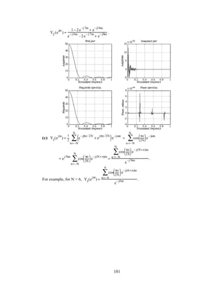
107. 0 0.2 0.4 0.6 0.8 1
-1
-0.5
0
0.5
1
ω/π
Real part
0 0.2 0.4 0.6 0.8 1
-0.5
0
0.5
1
1.5
ω/π
Imaginary part
0 0.2 0.4 0.6 0.8 1
0
0.2
0.4
0.6
0.8
1
ω/π
Magnitude spectrum
0 0.2 0.4 0.6 0.8 1
-4
-2
0
2
4
ω/π
Phase spectrum
M3.4 N = input('The length of the sequence = ');
k = 0:N-1;
gamma = -0.5;
g = exp(gamma*k);
% g is an exponential sequence
h = sin(2*pi*k/(N/2));
% h is a sinusoidal sequence with period = N/2
[G,w] = freqz(g,1,512);
[H,w] = freqz(h,1,512);
% Property 1
alpha = 0.5;
beta = 0.25;
y = alpha*g+beta*h;
[Y,w] = freqz(y,1,512);
% Plot Y and alpha*G+beta*H to verify that they are equal
% Property 2
n0 = 12; % S equence shifted by 12 samples
y2 = [zeros([1,n0]) g];
[Y2,w] = freqz(y2,1,512);
G0 = exp(-j*w*n0).*G;
% Plot G0 and Y2 to verify they are equal
% Property 3
w0 = pi/2; % the value of omega0 = pi/2
r=256; %the value of omega0 in terms of number of samples
k = 0:N-1;
103

108. y3 = g.*exp(j*w0*k);
[Y3,w] = freqz(y3,1,512);
k = 0:511;
w = -w0+pi*k/512; % creating G(exp(w-w0))
G1 = freqz(g,1,w');
% Compare G1 and Y3
% Property 4
k = 0:N-1;
y4 = k.*g;
[Y4,w] = freqz(y4,1,512);
% To compute derivative we need sample at pi
y0 = ((-1).^k).*g;
G2 = [G(2:512)' sum(y0)]';
delG = (G2-G)*512/pi;
% Compare Y4, delG
% Property 5
y5 = conv(g,h);
[Y5,w] = freqz(y5,1,512);
% Compare Y5 and G.*H
% Property 6
y6 = g.*h;
[Y6,w] = freqz(y6,1,512,'whole');
[G0,w] = freqz(g,1,512,'whole');
[H0,w] = freqz(h,1,512,'whole');
% Evaluate the sample value at w = pi/2
% and verify with Y6 at pi/2
H1 = [fliplr(H0(1:129)') fliplr(H0(130:512)')]';
val = 1/(512)*sum(G0.*H1);
% Compare val with Y6(129) i.e sample at pi/2
% Can extend this to other points similarly
% Parsevals theorem
val1 = sum(g.*conj(h));
val2 = sum(G0.*conj(H0))/512;
% Comapre val1 with val2
M3.5 N = 8; % Number of samples in sequence
gamma = 0.5;
k = 0:N-1;
x = exp(-j*gamma*k);
y = exp(-j*gamma*fliplr(k));
% r = x[-n] then y = r[n-(N-1)]
% so if X1(exp(jw)) is DTFT of x[-n], then
% X1(exp(jw)) = R(exp(jw)) = exp(jw(N-1))Y(exp(jw))
[Y,w] = freqz(y,1,512);
X1 = exp(j*w*(N-1)).*Y;
m = 0:511;
w = -pi*m/512;
X = freqz(x,1,w');
% Verify X = X1
% Property 2
k = 0:N-1;
y = exp(j*gamma*fliplr(k));
[Y,w] = freqz(y,1,512);
104

109. X1 = exp(j*w*(N-1)).*Y;
[X,w] = freqz(x,1,512);
% Verify X1 = conj(X)
% Property 3
y = real(x);
[Y3,w] = freqz(y,1,512);
m = 0:511;
w0 = -pi*m/512;
X1 = freqz(x,1,w0');
[X,w] = freqz(x,1,512);
% Verify Y3 = 0.5*(X+conj(X1))
% Property 4
y = j*imag(x);
[Y4,w] = freqz(y,1,512);
% Verify Y4 = 0.5*(X-conj(X1))
% Property 5
k = 0:N-1;
y = exp(-j*gamma*fliplr(k));
xcs = 0.5*[zeros([1,N-1]) x]+0.5*[conj(y) zeros([1,N-1])];
xacs = 0.5*[zeros([1,N-1]) x]-0.5*[conj(y) zeros([1,N-1])];
[Y5,w] = freqz(xcs,1,512);
[Y6,w] = freqz(xacs,1,512);
Y5 = Y5.*exp(j*w*(N-1));
Y6 = Y6.*exp(j*w*(N-1));
% Verify Y5 = real(X) and Y6 = j*imag(X)
M3.6 N = 8;
k = 0:N-1;
gamma = 0.5;
x = exp(gamma*k);
y = e xp(gamma*fliplr(k));
xev =0.5*([zeros([1,N-1]) x]+[y zeros([1,N-1])]);
xod = 0.5*([zeros([1,N-1]) x]-[y zeros([1,N-1])]);
[X,w] = freqz(x,1,512);
[Xev,w] = freqz(xev,1,512);
[Xod,w] = freqz(xod,1,512);
Xev = exp(j*w*(N-1)).*Xev;
Xod = exp(j*w*(N-1)).*Xod;
% Verify real(X)= Xev, and imag(X)= Xod
r = 0:511;
w0 = -pi*r/512;
X1 = freqz(x,1,w0');
% Verify X = conj(X1)
% real(X)= real(X1) and imag(X)= -imag(X1)
% abs(X)= abs(X1) and angle(X)= -angle(X1)
M3.7 N = input('The size of DFT to be computed =');
for k = 1:N
for m = 1:N
D(k,m) = exp(-j*2*pi*(k-1)*(m-1)/N);
end
end
diff = inv(D)-1/N*conj(D);
% Verify diff is N*N matrix with all elements zero
105

110. M3.8 (a)
clf;
N = input('The value of N = ');
k = -N:N;
y1 = ones([1,2*N+1]);
w = 0:2*pi/255:2*pi;
Y1 = freqz(y1, 1, w);
Y1dft = fft(y1);
k = 0:1:2*N;
plot(w/pi,abs(Y1),k*2/(2*N+1),abs(Y1dft),'o');
xlabel('Normalized frequency');ylabel('Amplitude');
(b) Add the statement y2 = y1 - abs(k)/N; below the statement y1 =
ones([1,2*N+1]); and replace y1, Y1, and Y1dft in the program with y2, Y2
and Y2dft, respectively.
(c) Replace the statement y1 = ones([1,2*N+1]); with y3 =
cos(pi*k/(2*N)); , and replace y1, Y1, and Y1dft in the program with y3, Y3
and Y3dft, respectively.
The plots generated for N = 3 is shown below where the circles denote the DFT samples.
(a) (b)
0 0.5 1 1.5 2
0
2
4
6
8
Normalized frequency
0 0.5 1 1.5 2
0
1
2
3
4
Normalized frequency
(c)
0 0.5 1 1.5 2
0
1
2
3
4
Normalized frequency
M3.9 g = [3 4 -2 0 1 -4];
106

111. h = [1 -3 0 4 -2 3];
x = [2+j*3 3-j -1+j*2 j*3 2+j*4];
v = [-3-j*2 1+j*4 1+j*2 5+j*3 1+j*2];
k = 0:4;
z = sin(pi*k/2);
y = 2.^k;
G = fft(g); H = fft(h); X = fft(x);
V = fft(v); Z = fft(z); Y = fft(y);
y1 = ifft(G.*H); y2 = ifft(X.*V); y3 = ifft(Z.*Y);
M3.10 N = 8; % N is length of the sequence(s)
gamma = 0.5;
k = 0:N-1;
g = exp(-gamma*k); h = cos(pi*k/N);
G = fft(g); H=fft(h);
% Property 1
alpha=0.5; beta=0.25;
x1 = alpha*g+beta*h;
X1 = fft(x1);
% Verify X1=alpha*G+beta*H
% Property 2
n0 = N/2; % n0 is the amount of shift
x2 = [g(n0+1:N) g(1:n0)];
X2 = fft(x2);
% Verify X2(k)= exp(-j*k*n0)G(k)
% Property 3
k0 = N/2;
x3 = exp(-j*2*pi*k0*k/N).*g;
X3 = fft(x3);
G3 = [G(k0+1:N) G(1:k0)];
% Verify X3=G3
% Property 4
x4 = G;
X4 = fft(G);
G4 = N*[g(1) g(8:-1:2)]; % This forms N*(g mod(-k))
% Verify X4 = G4;
% Property 5
% To calculate circular convolution between
% g and h use eqn (3.67)
h1 = [h(1) h(N:-1:2)];
T = toeplitz(h',h1);
x5 = T*g';
X5 = fft(x5');
% Verify X5 = G.*H
% Property 6
x6 = g.*h;
X6 = fft(x6);
H1 = [H(1) H(N:-1:2)];
T = toeplitz(H.', H1); % .' is the nonconjugate transpose
G6 = (1/N)*T*G.';
% Verify G6 = X6.'
107

112. M3.11 N = 8; % sequence length
gamma = 0.5;
k = 0:N-1;
x = exp(-gamma*k);
X = fft(x);
% Property 1
X1 = fft(conj(x));
G1 = conj([X(1) X(N:-1:2)]);
% Verify X1 = G1
% Property 2
x2 = conj([x(1) x(N:-1:2)]);
X2 = fft(x2);
% Verify X2 = conj(X)
% Property 3
x3 = real(x);
X3 = fft(x3);
G3 = 0.5*(X+conj([X(1) X(N:-1:2)]));
% Verify X3 = G3
% Property 4
x4 = j*imag(x);
X4 = fft(x4);
G4 = 0.5*(X-conj([X(1) X(N:-1:2)]));
% Verify X4 = G4
% Property 5
x5 = 0.5*(x+conj([x(1) x(N:-1:2)]));
X5 = fft(x5);
% Verify X5 = real(X)
% Property 6
x6 = 0.5*(x-conj([x(1) x(N:-1:2)]));
X6 = fft(x6);
% Verify X6 = j*imag(X)
M3.12 N = 8;
k = 0:N-1;
gamma = 0.5;
x = exp(-gamma*k);
X = fft(x);
% Property 1
xpe = 0.5*(x+[x(1) x(N:-1:2)]);
xpo = 0.5*(x-[x(1) x(N:-1:2)]);
Xpe = fft(xpe);
Xpo = fft(xpo);
% Verify Xpe = real(X) and Xpo = j*imag(X)
% Property 2
X2 = [X(1) X(N:-1:2)];
% Verify X = conj(X2);
% real(X) = real(X2) and imag(X) = -imag(X2)
% abs(X)= abs(X2) and angle(X) = -angle(X2)
108

113. M3.13 Using the M-file fft we obtain X[0] =13, X[1] = 12.8301 + j5.634, X[2] = −4 + j3.4641,
X[3] = −8+ j7, X[4] = 13+ j1.7321, X[5]= 4.1699 + j7.366, X[6]= –13, X[7] = 4.1699− j 7.366,
X[8] = 13− j1.7321, X[9] = −8 − j7, X[10]= − 4− j3.4641, X[11]= 12.8301− j5.634.
(a) X[0] = 13, (b) X[6] = – 13, (c) X[k] = 36,
k=0
11
∑ (d) e− j(4πk /6)
k=0
11
∑ X[k] = −48,
(e) X[k]
12
= 1500.
k=0
11
∑
M3.14 Using the M-file ifft we obtain x[0]= 2.2857, x[1] = −0.2643, x[2] = 0.7713, x[3]= −0.4754,
x[4]= −1.1362, x[6] = 1.6962, x[6] = 3.5057, x[7]= −0.8571, x[8] = 2.0763, x[9] = −0.6256,
x[10] =1.9748, x[11] =1.0625, x[12] =1.5224, x[13]= 0.4637,
(a) x[0] = 2.2857 , (b) x[7] = – 0.8571, (c) x[n]= 12,
n =0
13
∑ (d) e j(4πn /7)
x[n]= − 2 − j2,
n =0
13
∑
(e) x[n]
2
= 35.5714,
n =0
13
∑
M3.15
function y = overlapsave(x,h)
X = length(x); %Length of longer sequence
M = length(h); %length of shorter sequence
flops(0);
if (M > X) %Error condition
disp('error');
end
%clear all
temp = ceil(log2(M)); %Find length of circular convolution
N = 2^temp; %zero padding the shorter sequence
if(N > M)
for i = M+1:N
h(i) = 0;
end
end
m = ceil((-N/(N-M+1)));
while (m*(N-M+1) <= X)
if(((N+m*(N-M+1)) <= X)&((m*(N-M+1)) > 0))
for n = 1:N
x1(n) = x(n+m*(N-M+1));
end
end
if(((m*(N-M+1))<=0)&((N+m*(N-M+1))>=0)) %underflow adjustment
for n = 1:N
x1(n) = 0;
end
for n = m*(N-M+1):N+m*(N-M+1)
if(n > 0)
x1(n-m*(N-M+1)) = x(n);
end
end
end
109

114. if((N+m*(N-M+1)) > X) %overflow adjustment
for n = 1:N
x1(n) = 0;
end
for n = 1:(X-m*(N-M+1))
x1(n) =x (m*(N-M+1)+n);
end
end
w1 = circonv(h,x1); %circular convolution using DFT
for i = 1:M-1
y1(i) = 0;
end
for i = M:N
y1(i) = w1(i);
end
for j = M:N
if((j+m*(N-M+1)) < (X+M))
if((j+m*(N-M+1)) > 0)
yO(j+m*(N-M+1)) = y1(j);
end
end
end
m = m+1;
end
disp('Number of Floating Point Operations')
flops
%disp('Convolution using Overlap Save:');
y = real(yO);
function y = circonv(x1,x2)
L1 = length(x1); L2 = length(x2);
if L1 ~= L2,
error('Sequences of unequal lengths'),
end
X1 = fft(x1);
X2 = fft(x2);
X_RES = X1.*X2;
y = ifft(X_RES);
The MATLAB program for performing convolution using the overlap-save method is
h = [1 1 1]/3;
R = 50;
d = rand(1,R) - 0.5;
m = 0:1:R-1;
s = 2*m.*(0.9.^m);
x = s + d;
%x = [x x x x x x x];
y = overlapsave(x,h);
k = 0:R-1;
plot(k,x,'r-',k,y(1:R),'b--');
xlabel('Time index n');ylabel('Amplitude');
legend('r-', 's[n]','b--','y[n]');
110

115. 0 10 20 30 40 50
0
2
4
6
8
Time index n
s[n]
y[n]
M3.16 (a) Using the M-file roots we determine the zeros and the poles of G1(z) which are
given by z1 = −3.5616, z2 = −0.4500 + j0.7730, z3 = −0.4500 − j0.7730, z4 = 0.5616 , and
p1 = −1.0000 + j1.7321, p2 = −1.0000 − j1.7321, p3 = 0.6000 + j0.3742, p4 = 0.6000 − j0.3742.
Next using the M-file conv we determine the quadratic factors corresponding to the complex
conjugate zeros and poles resulting in the following factored form of G1(z):
G1(z) =
4
3
⋅
(1+ 3.5616z−1
)(1− 0.5616z−1
)(1+ 0.9z−1
+ 0.8z−2
)
(1+ 2z−1 + 4z−2)(1−1.2z−1 + 0.5z−2)
.
(b) Using the M-file roots we determine the zeros and the poles of G2(z) which are
given by z1 = −2, z2 = −1, z3 = −0.5, z4 = 0.3, and
p1 = −1.0482 + j1.7021, p2 = −1.0482 − j1.7021, p3 = −0.6094, p4 = −0.3942.
Next using the M-file conv we determine the quadratic factors corresponding to the complex
conjugate zeros and poles resulting in the following factored form of G2(z):
G2(z) =
2
5
⋅
(1+ 2z−1
)(1+z−1
)(1+ 0.5z−1
)(1− 0.3z−1
)
(1+ 0.6094 z−1)(1+ 0.3942 z−1)(1+ 2.0963z−1 + 3.9957z−2)
M3.17 Using Program 3_9 we arrive at we get
Residues
3.0000 2.0000
Poles
-1.0000 -0.3333
Constant
[]
Hence, Y1(z) =
3
1 + z−1 −
2
1+ 1
3
z−1
, which is same as that determined in Problem 3.98.
M3.18 (a) A partial-fraction expansion of Xa(z) =
4 − 3z−1
+ 3z−2
(z + 2)(z − 3)2 =
4z−3
− 3z−4
+ 3z−5
1− 4z−1
− 3z−2
+ 18z−3 .
using Program 3_9 we arrive at
Xa(z) = 0.2361z−2
− 0.1389z−1
+ 0.1667 −
0.1852
1− 3z−1 +
0.0741
(1− 3z−1
)2 −
0.125
1+ 2z−1 . Since the ROC is
111

116. given by z > 3, the inverse z-transform is a right-sided sequence and is thus given by
xa[n] = 0.2361δ[n − 2] − 0.1389δ[n − 1]+ 0.1667δ[n]
−0.1852(3)n
µ[n] + 0.0741n(3)n
µ[n] − 0.125(−2)n
µ[n].
A more compact solution is obtained by writing Xa(z) as Xa(z) = z−3 4 − 3z−1
+ 3z−2
1− 4z−1
− 3z−2
+ 18z−3





 ,
and making a partial-fraction expansion of the function inside the brackets:
Xa(z) = z−3 1
1− 3z−1 +
2
(1 − 3z−1
)2 +
1
1+ 2z−1





 = z−3 1
1 − 3z−1 +
1
1+ 2z−1





 + z−2 2z−1
(1− 3z−1
)2






The inverse z-trasform of the above function is given by
xa[n] = (3)n −3
µ[n − 3]+ (−2)n −3
µ[n − 3]+
2
3
(n − 2)(3)n−2
µ[n − 2]
= (3)n−3
(2n − 3) + (−2)n −3
[ ]µ[n − 3].
(b) Here the ROC is z < 2,hence, the inverse z-transform of
Xb (z) = z−3 1
1− 3z−1 +
1
1 + 2z−1





 + z−2 2z−1
(1− 3z−1
)2





 is thus given by
xb[n]= −(3)n −3
µ[−n + 2] − (−2)n−3
µ[−n + 2]−
2
3
(n − 2)(3)n−2
µ[−n +1]
= −(3)n−3
(2n − 3) − (−2)n−3
[ ]µ[−n + 2].
(c) In this case, the ROC is given by 2 < z < 3. Hence, the inverse z-transform of
Xc(z) = z−3 1
1− 3z−1 +
1
1+ 2z−1





 + z−2 2z−1
(1 − 3z−1
)2





 is thus given by
xc[n] = −(3)n−3
µ[−n + 2] + (−2)n −3
µ[n − 3]−
2
3
(n − 2)(3)n−2
µ[−n +1]
= −(3)n−3
(2n − 3)µ[−n + 2] + (−2)n −3
µ[n − 3].
M3.19 (a) Using the statement
[num,den] = residuez([10/4 -8/2],[-1/4 -1/2],0); we get
num = –3.5 –1.25 –0.25 and den = 1 0.75 0.125.
Hence the transfer function is given by X1(z) = −
3.5+ 1.25z−1
+ 0.25z−2
1+ 0.75z−1
+ 0.125z−2 .
(b) Using the statement [r,p,k]=residuez([–3 –1],[1 0 – 0.25]); we
first obtain a partial-fraction expansion of −
3+ z−1
1− 0.25z−2 which yields
r = – 2.5 0.5, p = 0.5 –0.5 and k = 0.
Therefore we can write
X2(z) = 3.5 −
2
1− 0.5z−1 −
2.5
1− 0.5z−1 +
0.5
1+ 0.5z−1 = 3.5 −
4.5
1− 0.5z−1 +
0.5
1+ 0.5z−1 . Next we use the
statement [num,den] = residuez([-4.5 0.5],[0.5 -0.5],3.5); which
112

117. yields num = –0.5 –2.5 –0.075 and den = 1 0 0.25. Therefore,
X2(z) = −
0.5+ 2.5z−1
+ 0.875z−2
1− 0.25z−2 .
(c) We first make a partial-fraction expansion of
3
1+ 0.81z−2 using the statement [r,p,k] =
residuez(3, [1 0 0.81],0); which yields
3
1+ 0.81z−2 =
1.5
1+ j0.9z−1 +
1.5
1− j0.9z−1 .
Hence, we can write X3(z) =
1.5
1+ j0.9z−1 +
1.5
1− j0.9z−1 −
4 / 3
1 + 2
3
z−1
+
5 / 9
1+ 2
3
z−1





2 . Using Program
3_10 we then obtain X3(z) =
2.2222 + 3.1111z−1
+ 0.70333z−2
− 0.72 z−3
1+ 1.3333z−1
+1.2544z−2
+1.08z−3
+ 0.36z−4 .
(d) We first make a partial-fraction expansion of
1
6
z−1
1+
5
6
z−1 +
1
6
z−2
using the statement
[r,p,k] = residuez([0 1 0]/6, [1 5/6 1/6],0); which yields
–
1
1+ 1
2
z−1
+
1
1+
1
3
z−1
. Hence, we can write X4(z) = 4 +
10/ 5
1+ 2
5
z−1
–
1
1+ 1
2
z−1
+
1
1+
1
3
z−1
. Using
Program 3_10 we then arrive at X4(z) =
6+ 6.7667z−1
+ 2.4z−2
+ 0.2667z−3
1+1.2333z−1 + 0.5z−2 + 0.0667 z−3 .
M3.20 (a) From Part (a) of M3.19 we observe X1(z) = −2 +
2.5
1+
1
4
z−1
–
4
1+ 1
2
z−1
. Hence its inverse
z-transform is given by x1[n]= −2δ[n]+ 2.5(−0.25)n
µ[n]– 4(−0.5)n
µ[n]. Evaluating for values of
n = 0,1,K we get x1[0] = −3.5, x1[1] = 1.375, x1[2] = −0.8438, x1[3] = 0.4609, x1[4] = −0.2402,
x1[5]= 0.1226, x1[6] = −0.0619, x1[7] = 0.0311, x1[8]= −0.0156, x1[9] = 0.0078
Using Program 3_11 we get
Coefficients of the power series expansion
Columns 1 through 6
-3.5000 1.3750 -0.8438 0.4609 -0.2402 0.1226
Columns 7 through 10
-0.0619 0.0311 -0.0156 0.0078
(b) From Part (b) of M3.19 we observe X2(z) = 3.5−
4.5
1− 0.5z−1 +
0.5
1+ 0.5z−1 . Hence, its inverse
z-transform is given by x2[n] = 3.5δ[n]− 4.5(0.5)n
µ[n]+ 0.5(−0.5)n
µ[n]. Evaluating for values
of n = 0,1,K we get x2[0]= −0.5, x2[1]= −2.5, x2 [2] = −0.1, x2[3] = −0.625, x2[4]= −0.25,
x2[5] = −0.1562, x2[6] = −0.0625, x2[7] = −0.0391, x2[8] = −0.0156, x2[9] = −0.0098,
Using Program 3_11 we get
113

118. Coefficients of the power series expansion
Columns 1 through 6
-0.5000 -2.5000 -0.1000 -0.6250 -0.2500 -0.1562
Columns 7 through 10
-0.0625 -0.0391 -0.0156 -0.0098
(c) From Part (c) of M3.19 we observe X3(z) =
3
1+ 0.81z−2 −
4 / 3
1+ 2
3
z−1
+
5 / 9
1+ 2
3
z−1





2 . Hence,
its inverse z-transform is given by
x3[n] = 3(0.9)n
cos(πn / 2)µ[n + 1]−
4
3
−
2
3






n
µ[n] +
5
9
−
3
2





 (n +1) −
2
3






n +1
µ[n + 1]
= 3(0.9)n
cos(πn / 2)µ[n]−
4
3
−
2
3






n
µ[n] +
5
9
(n + 1) −
2
3






n
µ[n]. Evaluating for values of n = 0,
1, . . . , we get x3[0]= 2.2222, x3[1]= 0.14815, x3[2]= –2.2819, x3[3] = −0.26337,
x3[4]= 2.2536, x3[5] = – 0.26337, x3[6] = −1.37, x3[7] = −0.18209, x3[8] = 1.4345,
x3[9] = − 0.10983. Using Program 3_11 we get
Coefficients of the power series expansion
Columns 1 through 6
2.2222 0.14815 -2.2819 -0.26337 2.2536 -0.26337
Columns 7 through 10
-1.37 -0.18209 1.4345 -0.10983
(d) From Part (d) of M3.19 we observe X4 (z) = 4 +
10 / 5
1 + 2
5
z−1
–
1
1+ 1
2
z−1
+
1
1 +
1
3
z−1
. Hence, its
inverse z-transform is given by x4[n]= 4δ[n] + 2(−2 / 5)n
µ[n]− (−1/ 2)n
µ[n] + (−1 / 3)n
µ[n].
Evaluating for values of n = 0,1,K we get x4[0] = 6, x4[1] = −0.6333, x4[2] = 0.1811,
x4[3]= −0.04, x4[4] = 0.0010, x4[5]= 0.0067, x4[6] = −0.0061, x4[7] = 0.0041, x4[8]= −0.0024,
x4[9] = 0.0014. Using Program 3_11 we get
Coefficients of the power series expansion
Columns 1 through 6
6.0000 -0.6331 0.1808 -0.0399 0.0011 0.0066
Columns 8 through 10
-0.0060 0.0040 -0.0024 0.0014
M3.21 % As an example try a sequence x = 0:24;
% calculate the actual uniform dft
% and then use these uniform samples
% with this ndft program to get the
% the original sequence back
% [X,w] = freqz(x,1,25,'whole');
% use freq = X and points = exp(j*w)
freq = input('The sample values = ');
points = input('Frequencies at which samples are taken = ');
L = 1;
114

119. len = length(points);
val = zeros(size(1,len));
L = poly(points);
for k = 1:len
if(freq(k) ~= 0)
xx = [1 -points(k)];
[yy, rr] = deconv(L,xx);
F(k,:) = yy;
down = polyval(yy,points(k))*(points(k)^(-len+1));
F(k,:) = freq(k)/down*yy;
val = val+F(k,:);
end
end
coeff = val;
115

120. Chapter 4 (2e)
4.1 If u[n] = z
n
is the input to the LTI discrete-time system, then its output is given by
y[n] = h[k]u[n − k]
k =−∞
∞
∑ = h[k]z
n−k
k =−∞
∞
∑ = z
n
h[k]z
−k
k=−∞
∞
∑ = z
n
H(z),
where H(z) = h[k]z
−k
k=−∞
∞
∑ . Hence u[n] = z
n
is an eigenfunction of the LTI discrete-time
system. If v[n] = z
n
µ[n] is the input to the system, then its output is given by
y[n] = h[k]v[n − k]
k =−∞
∞
∑ = z
n
h[k]µ[n − k]z
−k
k =−∞
∞
∑ = z
n
h[k]z
−k
k=−∞
n
∑ .
Since in this case the summation depends upon n, v[n] = z
n
µ[n] is not an eigenfunction of
an LTI discrete-time system.
4.2 h[n]= δ[n] − αδ[n − R]. Taking the DTFT of both sides we get H(ejω
) =1 − αe− jωR
.
Let α =| α | e
jφ
, then the maximum value of H(e
jω
) is 1+ α, and the minimum value of
H(e
jω
) is 1– α.
4.3 G(ejω
) = H(ejω
)( )
3
= (1− αe−jωR
)3
.
4.4 G(e
jω
) = α
n
n=0
M−1
∑ e
− jωn
=
1 − α
M
e
−jωM
1 −αe
− jω
. Note that G(e
jω
) = H(e
jω
), for α = 1. In order
to have the dc value of the magnitude response equal to unity the impulse response should be
multiplied by a factor of K, where K = (1− α)/(1− α
M
).
4.5 The group delay τ(ω) of an LTI discrete-time system with a frequency response H(e
jω
) =
H(e
jω
) e
jφ(ω)
, is given by τ(ω) = −
d(φ(ω))
dω
. Now,
dH(e
jω
)
dω
= e
jφ(ω)
dH(ejω
)
dω
+ j H(e
jω
) e
jφ(ω) dφ(ω)
dω
.
Hence, –j H(e
jω
) e
jφ(ω) dφ(ω)
dω
= e
jφ(ω)
dH(ejω
)
dω
–
d H(e
jω
)
dω
. Equivalently,
–
dφ(ω)
dω
=
e
jφ(ω)
j H(e
jω
) e
jφ(ω)
dH(e jω
)
dω
–
dH(e
jω
)
dω
jH(e
jω
)
=
1
j H(e
jω
)
dH(e jω
)
dω
+ j
dH(e
jω
)
dω
H(e
jω
)
.
The first term on the right hand side is purely imaginary. Hence,
116

121. τ(ω) = –
dφ(ω)
dω
= Re
j
d(H(e
jω
))
dω
H(e
jω
)














.
4.6 H(ejω
) = (a1 + a5 )cos2ω + (a2 + a4 )cosω + a3[ ]+ j (a1 – a5 )sin 2ω + (a2 – a4)sinω[ ]. Hence,
the frequency response will have zero phase for a1 = a5 , and a2 = a3.
4.7 H(ejω
) = a1 + a2e−jω
+ a3e−j2ω
+ a4e−j3ω
+ a5e− j4ω
+ a6e−j5ω
+ a7e−j6ω
= (a1ej3ω
+ a7e−j3ω
)e−j3ω
+ (a2ej2ω
+ a6e−j2ω
)e−j3ω
+ (a3ejω
+ a5e− jω
)e−j3ω
+ a4e−j3ω
. If
a1 = a7, a2 = a6 , and a3 = a5 , then we can write
H(ejω
) = 2(a1 + a7 )cos(3ω) + 2(a2 + a6 )cos(2ω) + 2(a3 + a5 )cos(ω) + a4[ ]e−j3ω
, which is seen
to have libear phase.
4.8 The frequency response of the LTI discrete-time system is given by
H(e
jω
) = a1e
jωk
+ a2e
jω(k−1)
+ a3e
jω(k−2)
+ a2e
jω(k−3)
+ a1e
jω(k−4)
= e
jω(k−2)
a1e
j2ω
+ a2e
jω
+ a3 + a2e
− jω
+ a1e
− j2ω
( )
= e
jω(k−2)
2a1cos(2ω) + 2a2 cos(ω) + a3( )
Hence for H(e
jω
) will be real for k = 2.
4.9 H1(ejω
) = α + e− jω
and H2(ejω
) =
1
1− βe− jω . Thus, H(ejω
) = H1(ejω
)H2 (ejω
) =
α + e− jω
1− βe− jω .
H(ejω
)
2
=
(α + e−jω
)(α + ejω
)
(1− βe−jω)(1−βejω)
=
α2
+ 2α cosω +1
1− 2βcosω + β2 . H(ejω
)
2
= 1, if α = −β.
4.10 Y(e
jω
) = X(e
jω
)
α
e
jarg X(e jω )
. Hence H(e
jω
) =
Y(e
jω
)
X(e
jω
)
= X(e
jω
)
(α−1)
. Since H(ejω
) is
real, it has zero-phase.
4.11 y[n] = x[n] + αy[n – R]. Y(ejω
) = X(ejω
)+ αe−jωR
Y(ejω
). Hence,
H(e
jω
) =
Y(e
jω
)
X(e
jω
)
=
1
1− αe−jωR . Maximum value of H(e
jω
) is 1/(1− | α |), and the
minimum value is 1/(1+ | α |). There are R peaks and dips in the range 0 ≤ ω < 2π. The
locations of peaks and dips are given by 1− α e−jωR
= 1± α, or e
−jωR
= ±
| α |
α
. The locations
of peaks are given by ω = ωk =
2π k
R
and the locations of dips are given by
ω = ωk =
(2π +1)k
R
, 0 ≤ k ≤ R − 1..
Plots of the magnitude and phase responses of H(e
jω
) for α = 0.8 and R = 6 re shown below:
117

122. 0 0.2 0.4 0.6 0.8 1 1.2 1.4 1.6 1.8 2
0.2
0.4
0.6
0.8
1
1.2
1.4
1.6
1.8
ω/π
Magnitude
0 0.2 0.4 0.6 0.8 1 1.2 1.4 1.6 1.8 2
-1
-0.8
-0.6
-0.4
-0.2
0
0.2
0.4
0.6
0.8
1
ω/π
Phase
4.12 A(e jω
) =
b0 + b1e−jω
+ b2e−j2ω
1+ a1e−jω
+ a2e−j2ω =
(b0ejω
+ b2e−jω
) + b1
(ejω
+ a2e−jω
) + a1
=
b1 + (b0 + b2 )cosω + j(b0 − b2 )sinω
a1 + (1+ a2 )cosω + j(1− a2 )sinω
. Therefore,
A(ejω
)
2
=
[b1 + (b0 + b2)]2
cos2
ω +(b0 − b2 )2
sin2
ω
[a1 + (1+ a2 )]2
cos2
ω + (1− a2 )2
sin2
ω
= 1. Hence, at ω = 0, we have
b1 + (b0 + b2) = ± a1 + (1+ a2 )[ ], and at ω = π / 2 we have b0 − b2 = ± 1− a2[ ].
Solution #1: Consider b0 − b2 = 1− a2 . Choose b0 =1,−b2 =1 − a2. and b2 = a2. Substituting
these values in b1 + (b0 + b2) = ± a1 + (1+ a2 )[ ], we have b1 = a1. In this case,
A(e jω
) =
1 + a1e−jω
+ a2e−j2ω
1 + a1e−jω
+ a2e−j2ω =1, a trivial solution.
Solution #2: Consider b0 − b2 = a2 −1. Choose b0 = a2, and b2 =1. Substituting these
values in b1 + (b0 + b2) = ± a1 + (1+ a2 )[ ], we have b1 = a1. In this case,
A(e jω
) =
a2 + a1e−jω
+ e−j2ω
1 + a1e−jω
+ a2e−j2ω .
4.13 From Eq. (2.17), the input-output relation of a factor-of-2 up-sampler is given by
y[n] =
x[n / 2], n = 0,± 2,± 4,K
0, otherwise.



The DTFT of the output is therefore given by
Y(ejω
) = y[n]e−jωn
n =−∞
∞
∑ = x[n / 2]
n=–∞
n even
∞
∑ e−jωn
= x[m]e−j2ωm
m=−∞
∞
∑ = X(e j2ω
) where X(e jω
) is the
DTFT of x[n].
118

123. 4.14
H(ej4ω
)
0 ↑ ↑ ↑ ↑
ω
π
0.2π
4
0.3π
4
2
π
4
π
2
3π
4
1.7π
4 1.8π
4
2.2π
4 2.3π
4
3.8π
4
3.7π
4
4.15 H(ejω
) = (0.4)n
n=0
∞
∑ e−jωn
=
1
1− 0.4e−jω . Thus, H(ejω
) =
1
1.16 − 0.8cosω
, and
arg H(ejω
){ }= θ(ω) = tan−1 0.4sinω
1− 0.4cosω





. H(e±jπ/ 4
) = 1.2067 m j0.4759. Therefore,
H(e±jπ / 4
) = 1.2972, and θ(± jπ / 4) = m 0.3757 radians.
Now for an input x[n] = sin(ωon)µ[n], the steady-state output is given by
y[n] = H(ejωo )sin ωon + θ(ωo )( ) which for ωo = π / 4 reduces to
y[n] = H(ejπ/ 4
)sin
π
4
n + θ(π/ 4)





 = 1.2972sin(
π
4
n − 0.3757).
4.16 H(e
jω
) = h[0] 1+ e
– j2ω
( )+ h[1]e
– jω
= e
–jω
2h[0]cosω + h[1]( ). Therefore, we require,
H(ej0.2
) = 2 h[0]cos(0.2)+ h[1] = 0, and H(ej0.5
) = 2h[0]cos(0.5)+ h[1] = 1. Solving these two
equations we get h[0]= − 4.8788 and h[1] = 9.5631.
4.17 (a) H(ejω
) = h0 + h1e− jω
− h1e− j3ω
− h0e− j4ω
= e− j2ω
h0 e j2ω
− e− j2ω
( )+ h0 e jω
− e− jω
( )[ ]
= je− j2ω
2h0 sin(2ω) + 2h1 sin(ω)[ ]. This implies, H(ejω
) = 2h0 sin(2ω) + 2h1 sin(ω). Thus,
H(ejπ/4
) = 2h0 sin(π / 2) + 2h1 sin(π / 4) = 0.5, and
H(ejπ/2
) = 2 h0 sin(π) + 2h1 sin(π / 2) = 1. Solving these two equations we get h0 = −0.1036,
and h1 = 0.5.
(b) H(ejω
) = je− j2ω
− 0.2072 sin(2ω) + sin(ω)[ ].
4.18 (a) H(ejω
) = h0 + h1e− jω
− h1e− j2ω
− h0e− j3ω
= e− j3ω/2
h0 e j3ω/ 2
− e− j3ω/ 2
( )+ h0 e jω/2
− e− jω/2
( )[ ]
= je− j3ω/2
2h0 sin(3ω / 2) + 2h1 sin(ω / 2)[ ]. This implies,
H(ejω
) = 2h0 sin(3ω / 2) + 2h1 sin(ω / 2). Thus, H(ejπ/4
) = 2h0 sin(3π / 8) + 2h1 sin(π / 8) = 1,
119

124. and H(ejπ/2
) = 2 h0 sin(3π / 4) + 2h1 sin(π / 4) = 0.5. Solving these two equations we get
h0 = −0.0381, and h1 = 0.7452.
(b) H(ejω
) = je− j3ω/2
−0.0762sin(3ω / 2) + 1.4904sin(ω / 2)[ ].
4.19 H(ejω
) = h0 + h1e− jω
+ h2e− j2ω
+ h1e− j3ω
+ h0e− j4ω
= e− j2ω
[h0(e j2ω
+ e− j2ω
) + h1(e jω
+ e− jω
) + h2 ] = e− j2ω
[2h0 cos(2ω) + 2h1 cos(ω) + h2 ].
This implies H(ejω
) = 2h0 cos(2ω) + 2h1 cos(ω) + h2 . Thus, we have
H(ej0.2
) = 2h0 cos(0.4) + 2h1 cos(0.2) + h2 = 0, H(ej0.5
) = 2h0 cos(1) + 2h1 cos(0.5) + h2 = 1,
H(ej0.8
) = 2h0 cos(1.6) + 2h1 cos(0.8) + h2 = 0. Solving these equations we get
h0 = −13.4866, h1 = 45.2280, h2 = − 63.8089.
4.20 H(ej0
) = 2, H(ejπ/ 2
) = 7 − j3, H(e jπ
) = 0. Using the symmetry property of the DTFT of a real
sequence, we observe H(ej3π/ 2
) = H * (ejπ/2
) = 7 + j3. Thus the 4-point DFT H[k] of the
length-4 sequence is given by H[k] = 2 7− j3 0 7 + j3[ ] whose 4-point inverse DFT yields
the impulse response coefficients {h[n]} = 4 2 −3 −1{ }, 0 ≤ n ≤ 3. Hence,
H(z) = 4 + 2z−1
− 3z−2
− z−3.
4.21 Now, for an anti-symmetric finite-length sequence, H(ej0
) = 0. Also, since the sequence is real,
H(ej3π/ 2
) = H * (ejπ/2
) = − 2 − j2. Thus the 4-point DFT H[k] of the length-4 sequence is
given by H[k] = 0 −2 + j2 8 −2 − j2[ ] whose 4-point inverse DFT yields the impulse
response coefficients {h[n]} = 1 −3 3 −1{ }, 0 ≤ n ≤ 3. Hence, H(z) = 1− 3z−1
+ 3z−2
− z−3.
4.22 (a) HA (ejω
) = 0.3− e−jω
+ 0.3e−2 jω
, HB(ejω
) = 0.3+ e−jω
+ 0.3e−2 jω
.
0 0.2 0.4 0.6 0.8 1
0
0.5
1
1.5
2
ω
Highpass Filter
0 0.2 0.4 0.6 0.8 1
0
0.5
1
1.5
2
ω
Lowpass Filter
(a) HA (e
jω
) (b) HB(e
jω
)
HA(e
jω
) is a highpass filter, whereas, HB(e
jω
) a lowpass filter.
(b) HC(e jω
) = HB(ejω
) = HA (ej(ω+π)
).
120

125. 4.23 y[n] = y[n −1] + 0.5 x[n] + x[n −1]{ }. Hence,
Y(e
jω
) = e
– jω
Y(e
jω
) + 0.5 X(e
jω
)+ e
– jω
X(e
jω
){ }, or, Htr (e
jω
) =
Y(e
jω
)
X(e
jω
)
= 0.5
1+ e
– jω
1– e
– jω







 .
4.24 y[n] = y[n − 2] +
1
3
x[n] + 4x[n −1] + x[n − 2]{ }. Hence, Hsim(e
jω
) =
1
3
1+ 4e
−jω
+ e
−2 jω
1− e
−2jω







 .
Note: To compare the performances of the Trapezoidal numerical integration formula with
that of the Simpson's formula, we first observe that if the input is xa(t) = ejwt, then the result
of integration is ya(t) = ya(t) =
1
jω
e
jωt
. Thus, the ideal frequency response H(ejw)is 1/jw.
Hence, we take the ratio of the frequency responses of the approximation to the ideal, and
plot the two curves as indicated below.
From the above plot it is eveident that the Simpson's formula amplifies high frequencies,
whereas, the Trapzoidal formula attenuates them. In the very low frequency range, both
formulae yield results close to the ideal. However, Simpson's formula is reasonably accurate
for frequencies close to the midband range.
4.25 A mirror-image polynomial A(z) of degree N satisfies the condition A(z) = z−N
A(z−1,
) and an
antimirror-image polynomial B(z) of degree N satisfies the condition B(z) = −z−N
B(z−1,
).
(a) Bmi(z) =
1
2
B(z) + z−N
B(z−1
){ }. Thus, z−N
Bmi (z−1
) =
1
2
z−N
B(z−1
) + B(z){ }= Bmi (z).
Likewise, B1i (z) =
1
2
B(z) − z−N
B(z−1
){ }. Thus, z−N
Bai(z−1
) =
1
2
z−N
B(z−1
) − B(z){ }= −Bai (z).
(b) H(z) =
Nmi (z) + Nai (z)
Dmi (z) + Dai(z)
. Thus, H(z−1
) =
Nmi (z−1
) + Nai(z−1
)
Dmi (z−1
) + Dai (z−1
)
=
Nmi (z) − Nai (z)
Dmi (z) − Dai (z)
. Hence,
H(z) + H(z−1
) =
Nmi (z) + Nai (z)
Dmi (z) + Dai (z)
+
Nmi (z) − Nai (z)
Dmi (z) − Dai (z)
= 2⋅
Dmi (z)Nmi(z) − Dai (z)Nai (z)
Dmi
2
(z) − Dai
2
(z)
, and
H(z) − H(z−1
) =
Nmi (z) + Nai (z)
Dmi (z) + Dai (z)
−
Nmi (z) − Nai (z)
Dmi (z) − Dai (z)
= 2⋅
Dmi (z)Nai (z) − Dai (z)Nmi (z)
Dmi
2
(z) − Dai
2
(z)
.
121

126. (c) Since H(z) is a real rational function of z−1
, H(z−1
)
z=ejω = H * (ejω
). Therefore,
Hre(ejω
) =
1
2
H(ejω
) + H *(ejω
){ }=
1
2
H(z) + H(z−1
){ }z=ejω
= Hev (z)z=ejω ,and
Hrim (ejω
) =
1
2j
H(ejω
) − H *(ejω
){ }=
1
2j
H(z) − H(z−1
){ }
z=ejω
= −jHod(z) z=ejω .
(d) H(z) =
3z2
+ 4z + 6
3z3
+ 2z2
+ z +1
and H(z−1
) =
3z−2
+ 4z−1
+ 6
3z−3
+ 2z−2
+ z−1
+1
=
6z3
+ 4z2
+ 3z
z3
+ z2
+ 2z + 3
. Thus,
Hev(z) =
1
2
H(z) + H(z−1
){ }=
1
2
3z2
+ 4z + 6
3z3
+ 2z2
+ z + 1
+
6z3
+ 4z2
+ 3z
z3
+ z2
+ 2z + 3








=
9z6
+ 13.5z5
+ 15z4
+16 z3
+15 z2
+ 13.5z + 9
3z6
+ 5z5
+ 9z4
+ 15z3
+ 9z2
+ 5z + 3
, and
Hod(z) =
1
2
H(z) − H(z−1
){ }=
1
2
3z2
+ 4z + 6
3z3
+ 2z2
+z + 1
−
6z3
+ 4z2
+ 3z
z3
+ z2
+ 2z + 3








=
− 9z6
− 10.5z5
− 8z4
+ 8z2
+ 10.5z + 9
3z6
+ 5z5
+ 9z4
+ 15z3
+ 9z2
+ 5z + 3
. Therefore,
Hre(ejω
) = Hev(z) z=ejω =
9cos(3ω) + 13.5cos(2ω) + 15cosω + 16
3cos(3ω) + 5cos(2ω) + 9cosω + 15
, and
Him (ejω
) = −jHod(z) z=ejω =
−9cos(3ω) −10.5cos(2ω) − 8cosω
3cos(3ω) + 5cos(2ω) + 9cosω + 15
.
4.26 Given the real part of a real, stable transfer function Hre(ejω
) =
ai
cos(iω)
i =0
N
∑
bi cos(iω)
i=0
N
∑
=
A(ejω
)
B(e jω )
, (1)
the problem is to determine the transfer function: H(z) =
P(z)
D(z)
=
pi
z−i
i =0
N
∑
di z−i
i =0
N
∑
.
(a) Hre(ejω
) =
1
2
H(ejω
) + H*(ejω
)[ ]=
1
2
H(e jω
)+ H(e− jω
)[ ] =
1
2
H(z)+ H(z−1
)[ ]z=ejω
.
Substituting H(z) = P(z)/D(z) in the above we get
Hre(ejω
) =
1
2
P(z)D(z−1
) + P(z−1
)D(z)
D(z)D(z−1) z=ejω
(2)
which is Eq. (4.241).
(b) Comparing Eqs. (1) and (2) we get B(ejω
) = D(z)D(z−1
)
z=ejω , (3)
A(ejω
) =
1
2
P(z)D(z−1
) + P(z−1
)D(z)[ ]z=e jω
. (4)
Now D(z) is of the form D(z) = K z−N
(z − zi
i=1
N
∏ ) (5)
122

127. where the zi 's are the roots of B(z) = B(ejω
)
ejω
=z
inside the unit circle and K is a scalar constant.
Putting ω = 0 in Eq. (3) we get B(1) = D(1)[ ]2
, or B(1) = K (1− zi )
i=1
N
∏ . Hence,
K = B(1) / (1− zi )
i=1
N
∏ . (6)
(c) By analytic continuation, Eq. (4) yields A(z) =
1
2
P(z)D(z−1
) + P(z−1
)D(z)[ ]. (7)
Substituting A(z) =
1
2
ai(zi
+ z−i
)
i=0
N
∑ and the polynomial forms of P(z) and D(z), we get
ai (zi
+ z−i
)
i=0
N
∑ = pi z−i
i=0
N
∑





 di zi
i=0
N
∑





 + pi zi
i =0
N
∑





 di z−i
i =0
N
∑





 and equating the
coefficients of (zi
+ z−i
)/ 2 on both sides, we arrive at a set of N+1 equations which can be solved
for the numerator coefficients pi of H(z).
For the given example, i.e., Hre(ejω
) =
1+ cos(ω) + cos(2ω)
17 − 8cos(2ω)
, we observe
A(z) = 1+
1
2
(z + z−1
) +
1
2
(z2
+ z−2
). (8)
Also, B(z) =17 − 4(z2
+ z−2
), which has roots at z = ±
1
2
and z = ±2. Hence,
D(z) = K z−2
(z −
1
2
)(z +
1
2
) = K(z2
−
1
4
)z−2
.
Aldo, from Eq. (6) we have K = 17 − 8 /(1− 1
4
) = 4, so that D(z) = 4− z−2
. (9)
Substituting Eqs. (8), (9) and P(z) = p0 + p1z−1
+ p2z−2
in Eq. (7) we get
1+ 1
2
(z + z−1
)+ 1
2
(z2
+ z−2
) = (p0 + p1z−1
+ p2z−2
)(4− z2
) + (p0 + p1z + p2z2
)(4 − z−2
)[ ].
Equating coefficients of (zi
+ z−i
)/ 2, i = 0, 1, 2, on both sides we get 4 p0 − p2 =1, 3p1 = 1,
4 p2 − p0 =1. Solving these equations we arrive at p0 = p1 = p2 = 1/ 3. Therefore,
H(z) =
1+ z−1
+ z−2
3(4 − z−2 )
.
4.27 G(z) = H
1+ α z−1
α + z−1





 . Thus, G(1) = H
1+ α
α +1





 = H(1). and G(−1) = H
1− α
α −1





 = H(−1).
4.28 H(z) = H1(z) H2 (z) + H3(z)[ ]= (3+ 2z−1
+ 4z−2
)
2
3
+
4
3





 +
2
5
+
8
5





 z−1
+
4
7
+
3
7





 z−2





= (3+ 2z−1
+ 4z−2
)(2 + 2z−1
+z−2
) = 6 + 10z−1
+ 15z−2
+10 z−3
+ 4z−4
.
123

128. 4.29 H(z) =
5 − 5z−1
+ 0.4z−2
+ 0.32 z−3
1+ 0.5z−1
− 0.34z−2
− 0.08z−3 = 5⋅
(1− 0.8z−1
)(1− 0.4z−1
)(1+ 0.2z−1
)
(1+ 0.8z−1
)(1− 0.5z−1
)(1+ 0.2z−1
)
= 5⋅
(1 − 0.8z−1
)(1− 0.4z−1
)
(1+ 0.8z−1
)(1 − 0.5z−1
)
,obtained using the M-file roots. The pole-zero plot obtained
using the M-file zplane is shown below. It can be seen from this plot and the factored form of
H(z), the transfer function is BIBO stable as all poles are inside the unit circle. Note also from the
plot the pole-zero cancellation at z = – 0.2.
-1 -0.5 0 0.5 1
-1
-0.5
0
0.5
1
Real part
4.30 H(z) =
5 −10.5z−1
+ 11.7z−2
+ 0.3z−3
− 4.4z−3
1+ 0.9z−1
− 0.76z−2
− 0.016z−3
− 0.096z−3
= 5⋅
(1+ 0.5z−1
)(1 − 0.8z−1
)(1− 1.8z−1
+ 2.2z−2
)
(1 +1.4486z−1
)(1− 0.6515z−1
)(1 + 0.1029z−1
+ 0.1017z−2
)
, obtained using the M-file
roots. The pole-zero plot obtained using the M-file zplane is shown below. It can be seen
from this plot and the factored form of H(z), the transfer function is unstable as there is a ploe
outside the unit circle at z = – 1.4486.
-1.5 -1 -0.5 0 0.5 1
-1
-0.5
0
0.5
1
Real part
4.31 H(z) =
−0.1z−1
+ 2.19 z−2
(1− 0.8z−1 + 0.4z−2 )(1+ 0.3z−1)
=
A + Bz−1
1− 0.8z−1 + 0.4z−2 +
C
1+ 0.3z−1 , where
124

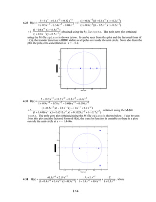
129. C =
−0.1z−1
+ 2.19 z−2
1− 0.8z−1 + 0.4z−2
z−1=−1/ 0.3
= 3, Thus,
A + B z−1
1− 0.8z−1 + 0.4z−2 =
−0.1z−1
+ 2.19z−2
(1− 0.8z−1 + 0.4z−2 )(1+ 0.3z−1)
−
3
1+ 0.3z−1 =
−3+ 3.2z−1
1− 0.8z−1 + 0.4z−2 Hence,
H(z) =
−3+ 3.2z−1
1− 0.8z−1 + 0.4z−2 +
3
1+ 0.3z−1 = −3
1−1.0667z−1
1− 0.8z−1 + 0.4z−2








+
3
1+ 0.3z−1 . Now, using Table
3.8 we observe r2
= 0.4 and r cosωo = 0.8. Therefore, r = 0.4 = 0.6325 and cosωo = 0.4 or
ωo = cos−1
0.4( )= 0.8861. Hence r sinωo = 0.4 sin(0.8861) = 0.4899. We can thus write
1−1.0667z−1
1− 0.8z−1 + 0.4z−2 =
1− 0.4z−1
1− 0.8z−1 + 0.4z−2 − 1.3609
0.4899z−1
1− 0.8z−1 + 0.4z−2





 . The inverse z-transform
of this function is thus given by (0.6325)n
cos(0.8861n)µ[n]− 1.3609(0.6325)n
sin(0.8861n)µ[n].
Hence, the inverse z-transform of H(z) is given by
h[n] = 3(0.6325)n
cos(0.8861n)µ[n]− 4.0827(0.6325)n
sin(0.8861n)µ[n]− 3(−0.3)n
µ[n].
4.32 (a) H(z) =
6 − z−1
1+ 0.5z−1 +
2
1− 0.4z−1 = k +
A
1+ 0.5z−1 +
2
1− 0.4z−1 where A = (6 − z−1
) z−1
=−2= 8
and k =
6 − z−1
1+ 0.5z−1
z−1=∞
= −2. Therefore, H(z) = −2+
8
1+ 0.5z−1 +
2
1− 0.4z−1 . Hence, the inverse
z-transform of H(z) is given by h[n] = −2δ[n]+ 8(−0.5)n
µ[n]+ 2(0.4)n
µ[n].
(b) x[n] =1.2(−0.2)n
µ[n]− 0.2(0.3)n
µ[n]. Its z-transform is thus given by
X(z) =
1.2
1+ 0.2z−1 −
0.2
1− 0.3z−1 =
1− 0.4z−1
(1+ 0.2z−1)(1− 0.3z−1)
, z > 0.3. Therefore,
Y(z) = H(z)X(z) =
6 − z−1
1+ 0.5z−1 +
2
1− 0.4z−1








1− 0.4z−1
(1+ 0.2z−1)(1− 0.3z−1)
=
8− 2.4z−1
+ 0.4z−2
(1+ 0.5z−1)(1− 0.4z−1)








1− 0.4z−1
(1+ 0.2z−1)(1− 0.3z−1)
=
8− 2.4z−1
+ 0.4z−2
(1+ 0.5z−1)(1+ 0.2z−1)(1− 0.3z−1)
, z > 0.5.
A partial-fraction expansion of Y(z) yields Y(z) =
15
1+ 0.5z−1 −
8
1+ 0.2z−1 +
1
1− 0.3z−1 . Hence,
the inverse z-transform of Y(z) is given by y[n] =15(−0.5)n
µ[n]− 8(−0.2)n
µ[n]+ (0.3)n
µ[n].
4.33 (a) h[n] =(0.8)n
µ[n] and x[n] = (0.5)n
µ[n]. Their z-transforms are given by
H(z) =
1
1− 0.8z−1 , z > 0.8 and X(z) =
1
1− 0.5z−1 , z > 0.5. The z-transform Y(z) of the output
125

130. y[n] is therefore given by Y(z) = H(z)X(z) =
1
(1− 0.8z−1)(1− 0.5z−1)
, z > 0.5. Its partial-fraction
expansion is given by Y(z) =
1
(1− 0.8z−1)(1− 0.5z−1)
=
8/ 3
1− 0.8z−1 −
5/ 3
1− 0.5z−1 . Hence, the inverse
z-transform of Y(z) is given by y[n] =
8
3
(0.8)n
µ[n]−
5
3
(0.5)n
µ[n].
(b) The z-transform Y(z) of the output y[n] is therefore given by
Y(z) = H(z)X(z) =
1
(1− 0.5z−1)2 , z > 0.5. Now, the inverse z-transform of
0.5z−1
(1− 0.5z−1)2 is
given by n(0.5)n
µ[n]. Thus, the inverse z-transform of
0.5
(1− 0.5z−1
)2 is given by
(n + 1)(0.5)n+1
µ[n + 1]. Hence, y[n] = (n + 1)(0.5)n
µ[n + 1]= (n + 1)(0.5)n
µ[n].
4.34 y[n] = 4(0.75)n
µ[n] and x[n] = 3(0.25)n
µ[n]. Their z-transforms are given by
Y(z) =
4
1− 0.75z−1 , z > 0.75 and X(z) =
3
1− 0.25z−1 , z > 0.25. Thus, the transfer function H(z)
is given by H(z) =
Y(z)
X(z)
=
4
3
1− 0.25z−1
1− 0.75z−1





 =
4
9
+
8/ 9
1− 0.75z−1 , z > 0.75. Hence, the impulse
response h[n] is given by h[n] =
4
9
δ[n]+
8
9
(0.75)n
µ[n].
4.35 (a) H(z) =
1
1− 0.8z−1 + 0.15z−2 =
1
(1− 0.5z−1)(1− 0.3z−1)
, z > 0.8.
(b) A partial-fraction expansion of H(z) yields H(z) =
2.5
1− 0.5z−1 −
1.5
1− 0.3z−1 . Hence,
h[n] = 2.5(0.5)n
µ[n] −1.5(0.3)n
µ[n].
(c) the step response s[n] is given by the inverse z-transform of
H(z)
1− z−1 =
1
(1− 0.5z−1)(1− 0.3z−1)(1−z−1)
, z >1. A partial-fraction expansion of
H(z)
1− z−1 yields
H(z)
1− z−1 =
2.8571
1−z−1 −
2.5
1− 0.5z−1 +
0.6429
1− 0.3z−1 . Hence, the step response is given by
s[n] = 2.8571µ[n]− 2.5(0.5)n
µ[n]+ 0.6429(0.3)n
µ[n].
4.36 Y(z) = [H0 (z)F0 (z)− H0(−z)F0(−z)]X(z). Since the output is a delayed replica of the input,
we must have H0(z)F0 (z) − H0 (−z)F0 (−z) = z–r. But H0(z) = 1+ α z−1
., hence
(1+α z−1
)F0 (z)− (1−α z−1
)F0 (−z) = z– r
. Let F0(z) = a0 + a1z
−1
. This impiles,
2(a0α + a1)z–1
= z–r
.
The solution is therefore, r = 1 and 2(a0α + a1) =1. One possible solution is thus a0 = 1/ 2,
α =1/ 2, and a1 = 1/ 4. Hence F0(z) = 0.25(1+ z
−1
).
126

131. 4.37 H0(z)F0 (z) = E0(z
2
) + z
−1
E1(z
2
)( ) R0 (z
2
)+ z
−1
R1(z
2
)( )
= E0(z
2
)R0 (z
2
)+ z
−1
(E0 (z
2
)R1(z
2
)+ E1(z
2
)R0(z
2
)( )+ z
−2
E1(z
2
)R1(z
2
). Thus,
H0(−z)F0(−z) = E0(z
2
)− z
−1
E1(z
2
)( ) R0 (z
2
) − z
−1
R1(z
2
)( )
= E0(z
2
)R0 (z
2
)− z
−1
E0(z
2
)R1(z
2
) + E1(z
2
)R0(z
2
)( )+ z
−2
E1(z
2
)R1(z
2
).
As a result, T(z)= H0(z)F0 (z) − H0 (−z)F0 (−z) = 2z
−1
E0 (z
2
)R1(z
2
)+ E1(z
2
)R0 (z
2
)( ).
Hence the condition to be satisfied by E0(z), E1(z), R0(z), R1(z) for the output to be a
delayed replica for input is E0(z
2
)R1(z
2
) + E1(z
2
)R0(z
2
) = 0.5z
−r
. (A)
(b) In Problem 4.36, E0(z) =1, E1(z) = 0.5, R0(z) = 0.5, R1(z) = 0.25. Thus,
E0(z2
)R1(z2
) + E1(z2
)R0(z2
) = 0.5.
Hence the condition of Eq. (A) is satisfied with r = 1.
(c) E0(z2
) = E1(z2
) = z–2
. Let R0 (z2
) = R1(z2
) = 0.25z–2
. r = 4 in this case. Hence
H(z) = z
–2
(1+ z
–1
) and F(z) =
1
4
z–2
(1– z–1
).
4.38 h[n] = h[N − n].
H(z) = h[n]z
–n
n=0
N–1
∑ = h[N – n]z
–n
n=0
N –1
∑ = h[k]z
–(N– k)
k =0
N –1
∑ = z
– N
H(z
–1
).
So if z = z0 is a root then so is z = 1/z0 . If G(z) = 1/H(z) then G(z) will have poles both
inside and outside the unit circle, and will hence be unstable.
4.39 D(z) = (0.5z +1)(z2
+ z + 0.6) = 0.5(z + 2)(z + 0.5− j0.5916)(z + 0.5+ j0.5916) . Since one of the
roots of D(z) is outside the unit circle at z = – 2, H(z) is unstable. To arrive at a stable, transfer
function G(z) such that G(ejω
) = H(ejω
), we multiply H(z) with an allpass function
A(z) =
0.5z + 1
z + 0.5
. Hence
G(z) = H(z)A(z) =
3z3
+ 2z2
+ 5
(0.5z + 1)(z2 + z + 0.6)






0.5z +1
z + 0.5





 =
3z3
+ 2z2
+ 5
(z + 0.5)(z2 + z + 0.6)
.
Now, H(z) =
3(z + 1.4545(z2
− 0.7878z + 1.1459)
(0.5z +1)(z2 + z + 0.6)
. Thus, there are 14 other transfer functions with
the same magnitude as H(ejω
) .
4.40 D(z) = (z + 3.1238)(z + 0.5762)(z − 0.2− j0.5568)(z − 0.2 + j0.5568). Since one of the roots of
D(z) is outside the unit circle at z = – 3.1238, H(z) is unstable. To arrive at a stable, transfer
function G(z) such that G(ejω
) = H(ejω
), we multiply H(z) with an allpass function
127

132. A(z) =
z + 3.1238
3.1238z +1
. Hence
G(z) = H(z)A(z) =
(z2
+ 2z − 3)(z2
− 3z + 5)
(z + 3.1238)(z + 0.5762)(z2 − 0.4z + 0.35)






z + 3.1238
3.1238z +1






=
(z2
+ 2z − 3)(z2
− 3z + 5)
(3.1238z +1)(z + 0.5762)(z2 − 0.4z + 0.35)
.
Now H(z) =
(z + 3)(z −1)(z2
− 3z + 5)
(z + 3.1238)(z + 0.5762)(z2 − 0.4z + 0.35)
. Hence there are ?? other transfer
functions with the same magnitude as H(ejω
) .
4.41 The transfer function of the simplest notch filter is given by
H(z) = (1− e
jωo
z−1
)(1− e
− jωo
z−1
) = 1− 2cosωo z−1
+ z−2
. In the steady-state, the output for an
input x[n]= cosωon is given by y[n] = H(e
jωo
) cos(ωon + θ(ωo )), (see Eq. (4.18)).
(a) Comparing H1(z) = 1+ z−2
with H(z) as given above we conclude cosωo = 0 or ωo = π / 2.
Here H1(e
jωo
) =1 − e
−j 2ωo
= 1− e−j π
=1 −1= 0. Hence, y[n] = H1(e
jωo
) cos(ωo n + θ(ωo )) = 0.
(b) Comparing H2(z) = 1−
3
2
z−1
+ z−2
with H(z) as given above we conclude cosωo = 3 / 4.
Here now H2(ejω
) =1 −
3
2
e− jω
+ e− j2ω
= 2cosωo −
3
2





 e−jω
= 0. Hence y[n] = 0.
(c) Comparing H3(z) = 1+ 2z−1
+ z−2
with H(z) as given above we conclude cosωo = −1/ 2.
Here now H2(ejω
) =1 + 2 e−jω
+ e−j2ω
= 2cosωo + 2( )e−jω
= 0. Hence y[n] = 0.
4.42 From the figure H0(z) =
Y0(z)
X(z)
= GL (z)GL(z
2
), H1(z) =
Y1(z)
X(z)
= GH (z)GL(z
2
),
H2(z) =
Y2(z)
X(z)
= GL (z)GH (z
2
), and H3(z) =
Y3(z)
X(z)
= GH (z)GH (z
2
),
128

133. 4.43 G(e
jω
) = HLP (e
j(π−ω)
). Since, HLP(e
jω
) =
1, 0 ≤ ω < ωc,
0, ωc ≤ ω < π,



G(e
jω
) =
0, 0 ≤ ω < π − ωc,
1, π − ωc ≤ ω < π.



Hence G(e
jω
) is a highpass filter with a cutoff frequency given by ω0 = π − ωc. Also, since
G(z) = HLP(–z), hence g[n] = (–1)nhLP[n].
4.44 G(z) = HLP (e
jωo z)+ HLP (e
−jωo z). Hence, g[n]= hLP [n]e
−jωon
+ hLP[n]e
jωon
=
2hLP[n]cos( ωo n). Thus, G(z) is a real coefficient bandpass filter with a center frequency at
wo and a passband width of 2ωp.
4.45 F(z) = HLP(e
jωo z) + HLP(e
−jωo z)+ HLP (z). Hence, f[n]= 1+ 2cos(ωon)( )hLP[n]. Thus,
F(z) is a real coefficient bandstop filter with a center frequency at wo and a stopband width of
π − 3ωp( )/ 2.
4.46
From the figure, V(z) = X(–z), U(z) = HLP(z)X(–z), and Y(z) = U(-z) = HLP(−z)X(z).
Hence Heq(z) = Y(z) / X(z) = HLP(−z) which is the highpass filter of Problem 4.41.
4.47
u0 [n] = 2x[n]cos(ωon) = x[n]e
jωo n
+ x[n]e
−jωon
or U0(e
jω
) = X(e
j(ω+ωo )
) + X(e
j(ω−ωo )
).
Likewise, U1(ejω
) = jX(ej(ω+ωo
)
)− jX(ej(ω−ωo
)
).
V0 (z) = HLP(z)X(ze
jωo ) + HLP(z)X(ze
−jωo ),
V1(z) = jHLP (z)X(zejωo ) − jHLP (z)X(ze−jωo ),
Y(z) =
1
2
V0(zejωo )+ V0(ze−jωo )( )+
j
2
V1(zejωo ) − V1(ze−jωo )( ) which after simplification
yields
129

134. Y(z) =
1
4
HLP(ze
jωo )X(ze
2jωo )+ HLP (ze
jωo )X(z)+ HLP (ze
−jωo )X(z)+ HLP (ze
−jωo )X(ze
−2jωo ){ }
−
1
4
HLP (ze
jωo )X(ze
2jωo ) − HLP(ze
jωo )X(z) − HLP (ze
−jωo )X(z) + HLP(ze
−jωo )X(ze
−2jωo ){ }
Hence Y(z) =
1
2
HLP(ze
jωo )+ HLP (ze
−jωo ){ }X(z), Therefore
Heq(z) =
Y(z)
X(z)
=
1
2
HLP (ze
jωo ) + HLP(ze
−jωo ){ }.
Thus the structure shown in Figure P4.6 implements the bandpass filter of Problem 4.42.
4.48
0 π 2π
−
π
M
π
M
ω
H0 (e
jω
)
0 π 2ππ
M
ω
H1(e
jω
)
2π
M
3π
M
0 π 2π
ω
3π
M
4π
M
H2(e
jω
)
0 π 2π
ω
−
2π
M
2(M − 1)π
M
↑
HM−1(ejω
)
The output of the k-th filter is a bandpass signals occupying a bandwidth of 2π/M and
centered at ω = kπ / M . In general, the k-th filter Hk(z) has a complex impulse response
130

135. generating a complex output sequence. To realize a real coefficient bandpass filter, one can
combine the outputs of Hk(z) and HM−k (z).
4.49 H0(z) =
1
2
(1+ z
−1
). Thus, H0(e
jω
) = cos(ω / 2). Now, G(z) = H0 (z)( )M
. Hence,
G(e
jω
)
2
= H0(e
jω
)
2M
= cos(ω / 2)( )2M
. The 3-dB cutoff frequency wc of G(z) is thus given
by cos(ωc / 2)( )2M
=
1
2
. Hence, ωc = 2cos
−1
(2
−1/ 2M
).
4.50 H1(z) =
1
2
(1− z
−1
). Thus, H1(e
jω
)
2
= sin
2
(ω/ 2). Let F(z) = H1(z)( )M
. Then
F(e
jω
)
2
= sin(ω / 2)( )2M
. The 3-dB cutoff frequency wc of F(z) is thus given
sin(ωc / 2)( )2M
=
1
2
, which yields ωc = 2 sin
−1
(2
−1/ 2M
).
4.51 HLP(z) =
1− α
2
1+ z
−1
1− αz
−1







 . Note that HLP(z) is stable if α < 1. Now,
α =
1− sin(ωc)
cos(ωc)
=
cos
2
(ωc / 2)+ sin
2
(ωc / 2) − 2sin(ωc / 2)cos(ωc / 2)
cos
2
(ωc / 2) − sin
2
(ωc / 2)
=
cos(ωc / 2) −sin(ωc / 2)
cos(ωc / 2)+ sin(ωc / 2)
=
1− tan(ωc / 2)
1+ tan(ωc / 2)
. (B)
If 0 ≤ ω < π then tan(ωc / 2) ≥ 0 hence α < 1.
4.52 From Eq. (B), α =
1− tan(ωc / 2)
1+ tan(ωc / 2)
, hence tan(ωc / 2) =
1− α
1+ α
.
4.53 (a) From Eq. (111b) we get α =
1− sin(0.4)
cos(0.4)
= 0.6629. Substituting this value of α in Eq.
(4.109) we arrive at HLP(z) =
0.1685(1+ z−1
)
1− 0.6629 z−1 .
(b) From Eq. (111b) we get α =
1− sin(0.3π)
cos(0.3π)
= 0.3249. Substituting this value of α in Eq.
(4.109) we arrive at HLP(z) =
0.3375(1+ z−1
)
1+ 0.3249 z−1 .
4.54 HHP(z) =
1+α
2
1− z
−1
1− αz
−1







 . Thus, HHP(e
jω
) =
1+ α
2
1− e
−jω
1− αe
−jω







 .
131

136. HHP (e
jω
)
2
=
1+ α
2




2
2− 2cos(ω)
1+ α
2
− 2α cos(ω)








. At 3-dB cutoff frequency ωc , HHP (e
jωc )
2
=
1
2
.
Hence,
1+ α
2




2 2− 2cos(ωc)
1+ α
2
− 2α cos(ωc)







 =
1
2
which yields cos(ωc) =
2α
1+ α
2 .
4.55 (a) From Eq. (111b) we get α =
1− sin(0.25)
cos(0.25)
= 0.7767. Substituting this value of α in Eq.
(4.112) we arrive at HHP(z) =
0.8884(1− z−1
)
1− 0.7767z−1 .
(b) From Eq. (111b) we get α =
1− sin(0.4π)
cos(0.4π)
= 0.1584. Substituting this value of α in Eq.
(4.112) we arrive at HHP(z) =
0.5792(1− z−1
)
1− 0.1584 z−1 .
4.56 H(z) =
1− z
−1
1− kz−1
. Hence, H(e
jω
)
2
=
(1− cosω)
2
+ sin
2
ω
(1− kcosω)
2
+ k
2
sin
2
ω
.
H(e
jω
)
2
=
(1 − cos(ω))
2
+ sin
2
(ω)
(1 − k cos(ω))2
+ k2
sin2
(ω)
=
2 − 2cosω
1+ k
2
− 2kcosω
.
Now H(e
jπ
)
2
=
4
(1+ k)
2 . Thus, the scaled transfer function is given by
H(z) =
1+ k
2
1− z
−1
1− kz
−1







 . A plot of the magnitude responses of the scaled transfer function for
k = 0.95, 0.9 and –0.5 are given below.
4.57 HBP(z) =
1− α
2
1− z
−2
1− β(1+ α)z
−1
+ αz
−2







 . Thus, HBP(e
jω
) =
1− α
2
1− e
−2 jω
1− β(1+ α)e
−jω
+ αe
−2 jω







 ,
HBP(ejω
)
2
=
1− α
2






2
2(1− cos2ω)
1+ β2(1+ α)2 + α2 + 2α cos2ω − 2β(1+ α)2 cosω
, which can be
simplified as HBP(ejω
)
2
=
(1− α)2
sin2
ω
(1+ α)2(cos ω − β)2 + (1− α)2 sin2 ω
.
At the center frequency wo, HBP(e
jωo )
2
= 1. Hence, (cosωo − β)2
= 0 or cosωo = β.
132

137. At the 3-dB bandedges w1 and w2, HBP(ejωi )
2
=
1
2
, i = 1, 2. This implies
(1+α)2
(cosωi − β)2
= (1− α)2
sin2
ωi , (C)
or sinωi = ±
1+ α
1− α





 cosωi − β( ), i = 1, 2. Since ω1 < ωo < ω2, sinω1 must have positive sign
whereas, sinω2 must have negative sign because otherwise, sinω2 < 0 for ω2 in (0, π).
Now, Eq. (C) can be rewritten as 2(1+ α2
)cos2
ωi − 2β(1+ α)2
cosωi +β2
(1+ α)2
−(1− α)2
= 0.
Hence, cosω1 + cosω2 = β
(1+ α)2
1+ α2 , and cosω1( ) cosω2( )=
β2
(1+ α)2
−(1− α)2
2(1+ α2 )
.
Denote ω3dB = ω2 − ω1. Then cos(ω3dB) = cosω2 cosω1 + sinω2 sinω1
= cosω2 cosω1 −
1+ α
1− α






2
cosω2 cosω1 + β2
− β(cos ω2 + cosω1)( ) =
2α
1+ α2 .
4.58 (a) Using Eq. (4.115) we get β = cos(0.45π) = 0.1564. Next from Eq. (4.116) we get
2α
1+ α2 = cos(0.2π) = 0.8090 or, equivalently α2
− 2.4721α +1 = 0. Solution of this quadratic
equation yields α =1.9626 and α = 0.5095. Substituting α =1.9626 and β = 0.1564 in Eq.
(4.113) we arrive at the denominator polynomial of the transfer function HBP(z) as
D(z) = (1− 0.4635z−1
+1.9626z−2
) = 1−(0.2317 + j1.3816)z−1
( )1 −(0.2317 − j1.3816)z−1
( ) which
has roots outside the unit circle making HBP(z) an unstable transfer function.
Next, substituting α = 0.5095 and β = 0.1564 in Eq. (4.113) we arrive at the denominator
polynomial of the transfer function HBP(z) as
D(z) = (1− 0.2361z−1
+ 0.5095z−2
) = 1−(0.1181+ j0.0704)z−1
( )1− (0.1181− j0.0704)z−1
( ) which
has roots inside the unit circle making HBP(z) a stable transfer function. The desired transfer
function is therefore HBP(z) =
0.2452(1− z−2
)
1− 0.2361z−1
+ 0.5095z−2 .
(b) Using Eq. (4.115) we get β = cos(0.6π) = − 0.3090. Next from Eq. (4.116) we get
2α
1 + α2 = cos(0.15π) = 0.8910 or, equivalently α2
− 2.2447α + 1= 0. Solution of this quadratic
equation yields α =1.6319 and α = 0.6128. Substituting α =1.6319 and β = − 0.3090 in Eq.
(4.113) we arrive at the denominator polynomial of the transfer function HBP(z) as
D(z) = (1+ 0.8133z−1
+1.6319z−2
) = 1 +(0.4066 + j1.2110)z−1
( ) 1+(0.4066 − j1.2110)z−1
( ) which
has roots outside the unit circle making HBP(z) an unstable transfer function.
Next, substituting α = 0.6128 and β = − 0.3090 in Eq. (4.113) we arrive at the denominator
polynomial of the transfer function HBP(z) as
D(z) = (1+ 0.4984z−1
+ 0.6128z−2
) = 1+(0.1181+ j0.7040)z−1
( )1+ (0.1181− j0.7040)z−1
( ) which
133

138. has roots inside the unit circle making HBP(z) a stable transfer function. The desired transfer
function is therefore HBP(z) =
0.1936(1− z−2
)
1+ 0.4984z−1
+ 6128z−2 .
4.59 HBS(z) =
1+ α
2






1− 2βz−1
+ z−2
1− β(1+ α)z−1 + αz−2 .
HBS(e jω
)
2
=
1+ α
2






2
2 + 4β2
− 8β cosω + 2cos2ω
1+ β2(1+ α)2 + α2 + 2α cos2ω − 2β(1+ α)2 cosω
, which can be
simplified as HBS(e jω
)
2
=
(1+ α)2
(cosω − β)2
(1+ α)2(cosω − β)2 +(1− α)2 sin2 ω
.
At the center frequency wo, HBS(e jωo )
2
= 0. Hence, (cosωo − β)2
= 0 or cosωo = β.
At the 3-dB bandedges w1 and w2, HBS(e jωi )
2
=
1
2
, i = 1, 2. This leads to Eq. (C) given
earlier Hence, as in the aolution of the previous problem ω3dB =
2α
1+ α2 .
4.60 (a) Using Eq. (4.115) we get β = cos(0.6π) = 0.3090. Next from Eq. (4.116) we get
2α
1 + α2 = cos(0.15π) = 0.8910 or, equivalently α2
− 2.2447α + 1= 0. Solution of this quadratic
equation yields α =1.6319 and α = 0.6128. Substituting α =1.6319 and β = 0.3090 in Eq.
(4.118) we arrive at the denominator polynomial of the transfer function HBS(z) as
D(z) = (1+ 0.8133z−1
+1.6319z−2
) = 1 +(0.4066 + j1.2110)z−1
( ) 1+(0.4066 − j1.2110)z−1
( ) which
has roots outside the unit circle making HBS(z) an unstable transfer function.
Next, substituting α = 0.6128 and β = 0.3090 in Eq. (4.113) we arrive at the denominator
polynomial of the transfer function HBS(z) as
D(z) = (1− 0.4984z−1
+ 0.6128z−2
) = 1+(0.2492 + j0.7421)z−1
( )1+ (0.2492− j0.7421)z−1
( ) which
has roots inside the unit circle making HBS(z) a stable transfer function. The desired transfer
function is therefore HBS(z) =
0.8064(1− 0.4984z−1
+ z−2
)
1 −0.4984 z−1
+ 6128z−2 .
(b) Using Eq. (4.115) we get β = cos(0.55π) = − 0.1564. Next from Eq. (4.116) we get
2α
1 + α2 = cos(0.25π) = 0.7071 or, equivalently α2
− 2.8284α +1= 0. Solution of this quadratic
equation yields α = 2.4142 and α = 0.4142. Substituting α = 2.4142 and β = − 0.1564 in Eq.
(4.118) we arrive at the denominator polynomial of the transfer function HBS(z) as
D(z) = (1+ 0.5341z−1
+ 2.4142 z−2
) = 1+ (0.2671+ j1.5307)z−1
( )1+ (0.2671− j1.5307)z−1
( ) which
has roots outside the unit circle making HBS(z) an unstable transfer function.
Next, substituting α = 0.4142 and β = 0.3090 in Eq. (4.113) we arrive at the denominator
polynomial of the transfer function HBS(z) as
134

139. D(z) = (1+ 0.2212z−1
+ 0.4142 z−2
) = 1+ (0.1106+ j0.6344)z−1
( )1+ (0.1106− j0.6344)z−1
( ) which
has roots inside the unit circle making HBS(z) a stable transfer function. The desired transfer
function is therefore HBS(z) =
0.7071(1+ 0.3129z−1
+ z−2
)
1 +0.2212z−1
+ 0.4142z−2 .
4.61
(1− α)
2
(1+ cosωc)
2(1+ α
2
− 2αcosωc)
= 2
−1/ K
. Let B = 2
(K−1)/K
. Simplifying this equation we get
α
2
(cosωc +1− B)− 2α(1+ cosωc − Bcosωc) +1+ cosωc − B = 0
Solving the above quadratic equation for α we obtain
α =
2(1+ (1− B)cosωc)± 4(1+ (1− B)cosωc)
2
− 4(1+ cosωc − B)
2
2(1+ cosωc − B)
=
1+ (1− B)cosωc( )± (2 + 2cosωc − B − Bcosωc) B(1− cosωc)( )
(1+ cosωc − B)
=
1+ (1− B)cosωc ± sin ωc 2B − B
2
(1+ cosωc − B)
. For stability we require α < 1, hence the desired
solution is α =
1+ (1− B)cosωc −sin ωc 2B − B
2
(1+ cosωc − B)
.
4.62 HHP(z) =
1+α
2
1− z
−1
1− αz
−1







 . HHP (e
jω
)
2
=
1+ α
2




2
1− e
−jω
1− αe
−jω
2
HHP (e
jω
)
2K
=
1+ α
2




2K
1− e
−jω
1− αe
−jω
2K
=
1+ α
2




2K
2K
1− cosω( )K
1+ α2 − 2α cosω( )K
At the 3-dB cut off frequency ωc , HHP (e
jωc )
2K
=
1
2
. Let B = 2
(K −1) / K
. Simplifying the
above equation we get α
2
(1− cosωc − B)+ 2α(1− cosωc + Bcosωc) +1− cosωc − B = 0.
Hence, α =
−2(1− cosωc + Bcosωc) ± 2 (1− cosωc + Bcosωc)
2
− (1− cosωc − B)
2
2(1− cosωc − B)
For HHP(z) to be stable, we require α < 1, hence the desired solution is
α =
sinωc 2B − B
2
− (1− cosωc + Bcosωc)
(1− cosωc − B)
.
4.63 H1(z) = H(−z). H1(e
jω
) = H(e
(π−ω)
). If H(e
jω
) is a lowpass filter with a passband edge at
wp, then H1(e
jω
) ≈
1, if π – ωp ≤ ω < π,
0, if 0 ≤ ω < π – ωp ,




hence H1(e
jω
) is a highpass filter.
135

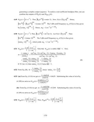
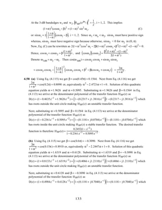
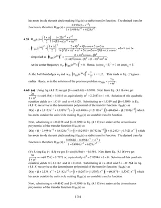
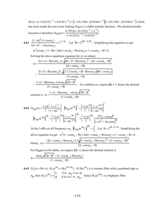
140. Now, h1[n] = (−1)
n
h[n]. The passband edge of the highpass filter is given by
ωp,HP = π − ωp,LP , and the stopband edge is given by ωs,HP = π − ωs,LP .
4.64 HLP(z) =
1− α
2
1+ z
−1
1− αz
−1







 , GHP(z) =
1− α
2
1− z
−1
1+ αz
−1







 . Let β = −α , hence
GHP(z) =
1+ β
2
1− z
−1
1− βz
−1







 . Therefore ωc = cos
−1
(β) = cos
−1
(−α).
4.65 The magnitude responses of H(z), H(–z), H(z2) and H(–z2) are shown below.
The magnitude responses of H(–z)H(z2), H(–z)H(z2), and H(z)H(–z2) are shown below.
4.66 The magnitude responses of H(zM) (solid line) and F1(z) (dashed line) are shown below:
Hence G1(z) = H(zM)F1(z) is a lowpass filter with unity passband magnitude and passband
edge at wp/M, and a stopband edge at ws/M.
The magnitude responses of H(zM) (solid line) and F2(z) (dashed line) are shown below:
136

141. Hence G2(z) = H(zM)F2(z) is a bandpass filter with unity passband magnitude and passband
edges at (2π–wp)/M and (2π+wp)/M, and a stopband edges at (2π–ws)/M and (2π+ws)/M.
4.67 v[n] = x[–n] * h[n], and u[n] = v[–n] = x[n] * h[–n]. Hence y[n] = (h[n] + h[–n]) * x[n].
Therefore G(e
jω
) = H(e
jω
) + H
*
(e
jω
). Hence the equivalent transfer function G(e
jω
) is real
and has zero phase.
4.68 From Eq. (4.81) we observe that the amplitude response
(
H(ω) of a Type 1 FIR transfer
function is a function of cos(ωn). Thus,
(
H(ω + 2πk) will be a function of
cos (ω + 2πk)n[ ]= cos(ωn + 2πkn) = cos(ωn)cos(2πkn)−sin(ωn)sin(2πkn) = cos(ωn),and hence
(
H(ω) is a periodic function in ω with a period 2π.
Likewise, from Eq. (4.91) we note that the amplitude response
(
H(ω) of a Type 3 FIR transfer
function is a function of sin(ωn). Thus,
(
H(ω + 2πk) will be a function of
sin (ω + 2πk)n[ ]= sin(ωn + 2πkn) = sin(ωn)cos(2πkn)−cos(ωn)sin(2πkn) = sin(ωn), and hence
(
H(ω) is a periodic function in ω with a period 2π.
Next, from Eq. (4.86) we observe that the amplitude response
(
H(ω) of a Type 2 FIR transfer
function is a function of cos ω(n −
1
2
)





 . Thus,
(
H(ω + 4πk) will be a function of
cos (ω + 4πk)(n −
1
2
)





 = cos ω(n −
1
2
) + 4πk(n −
1
2
)






= cos ω(n −
1
2
)





 cos 4πk(n −
1
2
)





 − sin ω(n −
1
2
)





 sin 4πk(n −
1
2
)





 = cos (ω + 4πk)(n −
1
2
)





 as
cos 4πk(n −
1
2
)





 = 1 and sin 4πk(n −
1
2
)





 = 0. ence
(
H(ω) is a periodic function in ω with
a period 4π.
Finally, from Eq. (4.96) we observe that the amplitude response
(
H(ω) of a Type 4 FIR transfer
function is a function of sin ω(n −
1
2
)





 . Thus,
(
H(ω + 4πk) will be a function of
sin (ω + 4πk)(n −
1
2
)





 = sin ω(n −
1
2
) + 4πk(n −
1
2
)






= sin ω(n −
1
2
)





 cos 4πk(n −
1
2
)





 − cos ω(n −
1
2
)





 sin 4πk(n −
1
2
)





 = sin ω(n −
1
2
)





 as
137

142. cos 4πk(n −
1
2
)





 = 1 and sin 4πk(n −
1
2
)





 = 0. ence
(
H(ω) is a periodic function in ω with
a period 4π.
4.69 The zeros given are at z1 = − 0.5, z2 =0.3+ j0.5, z3 = −
1
2
+ j
3
2
. The remaining zeros are at
z4 = 1/ z1 = − 2, z5 = z2 * = 0.3 − j0.5, z6 =1 / z5 = 0.12 − j0.1993, z7 = z6* = 0.12 + j0.1993, and
z8 = z3* = −
1
2
+ j
3
2
. Hence, H(z) = (1− zii=1
8
C z−1
)
= 1− 1.1353z−1
+ 0.5635z−2
+ 5.6841z−3
+ 4.9771z−4
+ 5.6841z−5
+ 0.5635z−6
−1.1353z−7
+ z−8
.
4.70 The zeros given are at z1 = 3, z2 = j0.8, z3 = j. The remaining zeros are at z4 = 1/ z1 = 1/ 3,
z5 = z2 * = − j0.8, z6 = z3*= −j, z7 =1 / z2 = −j 0.125, z8 = z7 *= j0.125, and z9 = −1. Hence,
H(z) = (1− zii=1
9
C z−1
)
= 1− 2.3333z−1
+ 0.8692z−2
− 6.4725z−3
− 4.27z−4
− 4.27z−5
− 6.4725z−6
+0.8692z−7
− 2.3333z−8
+ z−8
.
4.71 The zeros given are at z1 = − 0.3 + j0.5; z2 = j0.8; and z3 = − 0.3. The remaining zeros are at
z4 = z1* = − 0.3 − j0.5; z5 = 1 / z1 = − 0.8824 − j1.4786; z6 = z5*= − 0.8824 + j1.4786;
z7 = z2* = − j0.8; z8 = 1/ z7 = −j1.25; z9 = z8 *= j1.25; z10 =1 / z3 = −3.3333; z11 = 1; and
z12 = −1. Hence, H(z) = (1− zii=1
12
C z−1
) = 1+ 5.998z−1
+15.1343z−2
+ 27.7107z−3
+ 29.4822z−4
+ 23.4343z−5
− 23.4343 z−7
− 23.4343z−8
−29.4822z−9
−27.7107z−10
−15.1343z−11
− 5.998z−12
− z−13
.
4.72 The zeros given are at z1 = −1.2 + j1.4; z2 =
1
2
+ j
3
2
; z3 =
1
4
+ j
15
4
. The remaining zeros
are at z4 = z1* = −1.2 − j1.4; z5 = 1 / z1 = − 0.3529 − j0.4181; z6 = z5*= − 0.3529 + j0.4181;
z7 = z2* =
1
2
− j
3
2
; z8 = z3* =
1
4
− j
15
4
, and z9 =1. Hence, H(z) = (1− zii=1
9
C z−1
)
= 1+ 0.6059 z−1
+ 1.6235z−2
− 1.9412z−3
+ 4.8647z−4
− 4.8647 z−5
+ 1.9412z−6
−1.6235z−7
− 0.6059z−8
− z−9
.
4.73 H(z) = h[n]z−n
n =0
N
∑ , and H(ejω
) = h[n]e−jωn
n =0
N
∑ . The frequency response will exhibit
generalized linear phase if it can be expressed in the form H(ejω
) =
(
H(ω)e−jαω
e− jβ
, where
(
H(ω), the amplitude function, is a real function of ω , and α and β are constants.
138

143. We need to examine the case when the order N is even and when N is odd separately. Without
any loss of generality, assume first N = 5. Then H(z) = h[n]z−n
n =0
5
∑ , and
H(ejω
) = h[0] + h[1]e−jω
+ h[2]e−j2ω
+ h[3]e−j3ω
+ h[4]e−j4ω
+ h[5]e−j5ω
= e−j5ω/2
h[0]ej5ω/ 2
+ h[5]e−j5ω /2
+ h[1]e j3ω /2
+ h[4]e−j3ω/ 2
+ h[2]ejω/2
+ h[3]e− jω/ 2
[ ]
= e−j5ω/2
(h[0]+ h[5]) cos(5ω / 2) + (h[1]+ h[4])cos(3ω / 2) + (h[2]+ h[3]) cos(ω / 2)[ ]
+ je−j5ω/2
(h[0]− h[5])sin(5ω / 2) + (h[1]− h[4])sins(3ω / 2) + (h[2]− h[3]) sin(ω / 2)[ ].
Note from the above expression that if h[n]= h[5 − n], 0 ≤ n ≤ 5, then we have
H(ejω
) = e−j5ω/ 2 (
H(ω), where
(
H(ω) = 2h[0]cos(5ω / 2) + 2h[1]cos(3ω / 2) + 2h[2cos(ω / 2),
which is a real function of ω , and as a result, H(ejω
) has linear phase. Alternately, if
h[n]= − h[5 − n], 0 ≤ n ≤ 5, then we have H(ejω
) = je−j5ω/ 2 (
H(ω) = e−j5ω/2
e jπ/2 (
H(ω), where
(
H(ω) = 2h[0]sin(5ω / 2) + 2h[1]sin(3ω / 2) + 2h[2sin(ω / 2), which is a real function of ω , and
as a result, H(ejω
) has generalized linear phase.
Next, we assume first N = 6. Then H(z) = h[n]z−n
n =0
6
∑ , and
H(ejω
) = h[0] + h[1]e−jω
+ h[2]e−j2ω
+ h[3]e−j3ω
+ h[4]e−j4ω
+ h[5]e−j5ω
+ h[6]e−j6ω
= e−j3ω
h[0]ej3ω
+ h[6]e−j3ω
+ h[1]ej2ω
+ h[5]e−j2ω
+ h[2]ejω
+ h[4]e−jω
+ h[3][ ]
= e−j3ω
(h[0]+ h[6])cos(3ω) + (h[1]+ h[5]) cos(2ω) + (h[2]+ h[4])cos(ω) + h[3][ ]
+ e−j3ω
(h[0]− h[6]) sins(3ω) + (h[1]− h[5]) sin(2ω) + (h[2]− h[4])sin(ω)[ ].
Note from the above expression that if h[n]= h[6 − n], 0 ≤ n ≤ 6, then we have
H(ejω
) = e−j3ω (
H(ω), where
(
H(ω) = 2h[0]cos(3ω) + 2h[1]cos(2ω) + 2h[2]cos(ω) + h[3]
which is a real function of ω , and as a result, H(ejω
) has linear phase. Alternately, if
h[n]= − h[6 − n], 0 ≤ n ≤ 6, then we have H(ejω
) = je−j3ω (
H(ω) = e−j3ω
ejπ/2 (
H(ω), where
(
H(ω) = 2h[0]sin(3ω) + 2 h[1]sin(2ω) + 2h[2]sins(ω) which is a real function of ω , and as a
result, H(ejω
) has generalized linear phase.
4.74 (a) H2(z) is linear-phase (also can be seen from the symmetric impulse response).
(b) H3(z) is minimum-phase as all its zeros are inside the unit circle.
(c) H5(z) is maximum-phase as all its zeros are outside the unit circle.
4.75 G1(z) = (6 − z
−1
− 12z
−2
)(2 + 5z
−1
) = 30(1−
3
2
z
−1
)(1+
4
3
z
−1
)(
2
5
+ z
−1
).
(a) The other transfer functions having the same magnitude response are:
139

144. (i) H1(z) = 30(−
3
2
+ z
−1
)(1+
4
3
z
−1
)(
2
5
+ z
−1
), (ii) H2(z) = 30(1−
3
2
z
−1
)(
4
3
+ z
−1
)(
2
5
+ z
−1
),
(iii) H3(z) = 30(1−
3
2
z
−1
)(
4
3
+ z
−1
)(1+
2
5
z
−1
), (iv) H4 (z) = 30(–
3
2
+ z
−1
)(
4
3
+ z
−1
)(1+
2
5
z
−1
),
(v) H5(z) = 30(–
3
2
+ z
−1
)(1+
4
3
z
−1
)(1+
2
5
z
−1
), (vi) H6(z) = 30(1−
3
2
z
−1
)(1+
4
3
z
−1
)(1+
2
5
z
−1
),
(vii) H7(z) = 30(–
3
2
+ z
−1
)(
4
3
+ z
−1
)(1+
2
5
z
−1
).
(b) H7(z) has a minimum phase response, and G1(z) has a maximum phase response.
(c) The partial energy of the impulse responses of each of the above transfer functions for
different values of k are given by
k = 0 k = 1 k = 2 k = 3 k = 4
G1(z) 144 928 1769 5369 5369
H1(z) 324 3573 3769 5369 5369
H2 (z) 256 1040 3344 5369 5369
H3(z) 900 949 4793 5369 5369
H4(z) 576 4420 4469 5369 5369
H5(z) 2025 4329 5113 5369 5369
H6(z) 1600 1796 5045 5369 5369
H7(z) 3600 4441 5225 5369 5369
The partial energy remains the same for values of k > 2. From the table given above it can be
seen that hi[m]
2
m=0
k
∑ ≤ h7[m]
2
,
m=0
k
∑ and hi[m]
2
m=0
∞
∑ = h7[m]
2
,
m=0
∞
∑ i = 1, 2, . . . , 7.
4.76 A maximum-phase FIR transfer function has all zeros outside the unit circle, and hence, the
product of the roots is necessarily greater than 1. This implies that only those FIR transfer
functions which have the coefficient of the highest power in z–1 (z–6 in the present case) greater
than 1 can have maximum phase. Thus only H1(z) and H3(z) can be maximum-phase transfer
functions. Also, maximum-phase transfer functions will have minimum partial-energy (as
indicated in the solution of Problem 4.65). Hence, H1(z) is a maximum-phase transfer function
since it has the smallest constant term in comparison with that of H3(z).
Likewise, a minimum-phase FIR transfer function is characterized by: (1) largest constant term,
and (2) the value of the coefficient of the highest power of z–1 being less than 1. In the present
problem, it can be seen that H2(z) satisfies these two conditions and, is hence, a minimum-phase
transfer function.
Total no. of length-7 sequences having the same magnitude response is 27. Thus, there exist
123 other sequences with the same magnitude responses as those given here.
4.77 (a) Type 1: {h[n]} = a b c d c b a{ },
(b) Type 2: {h[n]} = a b c d d c b a{ },
140

145. (c) Type 3: {h[n]} = a b c d 0 −d −c −b −a{ },
(d) Type 4: {h[n]} = a b c d −d −c −b −a{ }.
4.78 (a) Type 1: H(z) = −1 − 2z−1
− 4z−2
+ 5z−3
+ 6z−4
+ 5z−5
− 4z−6
− 2z−7
− z−8
. From the zero
plot obtained using the M-file zplane it can be seen that complex-conjugate zero pairs inside
and outside the unit circle appear in mirror-image symmetry, complex conjugate zero-pair on
the unit circle appear singly and the zero at z = 1 is of order 2, verifying the observations of
Section 4.4.4 of text.
(b) Type 2: H(z) = −1 − 2z−1
− 4z−2
+ 5z−3
+ 6z−4
+ 6z−5
+ 5z−6
− 4z−7
− 2z−8
− z−9
. From
the zero plot obtained using the M-file zplane it can be seen that complex-conjugate zero
pair inside and outside the unit circle appear in mirror-image symmetry, complex conjugate
zero-pair on the unit circle appear singly, there is a zero at z =–1, and the zeros on the real axis
exhibit mirror-image symmetry, verifying the observations of Section 4.4.4 of text.
(c) Type 3: H(z) = −1 − 2z−1
− 4z−2
+ 5z−3
+ 6z−4
− 6z−6
− 5z−7
+ 4z−8
+ 2z−9
+ z−10
. From
the zero plot obtained using the M-file zplane it can be seen that complex-conjugate zero
pair inside and outside the unit circle appear in mirror-image symmetry, complex conjugate
zero-pair on the unit circle appear singly, there is a zero at z =–1 and at z = 1, verifying the
observations of Section 4.4.4 of text.
(d) Type 4: H(z) = −1 − 2z−1
− 4z−2
+ 5z−3
+ 6z−4
− 6z−5
− 5z−6
+ 4z−7
+ 2z−8
+z−9
. From
the zero plot obtained using the M-file zplane it can be seen that complex-conjugate zero
pair inside and outside the unit circle appear in mirror-image symmetry, complex conjugate
zero-pair on the unit circle appear singly, and there is a zero at z = 1, verifying the
observations of Section 4.4.4 of text.
4.79 H1(z) is of Type 1 and hence, it has a symmetric impulse response of odd length 2n+1. Let α
be the constant term of H1(z). Then, the coefficient of the highest power of z−1
of H1(z) is
also α .
H2(z) is of Type 2 and hence, it has a symmetric impulse response of even length 2m. Let β
be the constant term of H2(z) . Then, the coefficient of the highest power of z−1
of H2(z) is
also β.
H3(z) is of Type 3 and hence, it has an anti-symmetric impulse response of odd length 2r+1.
Let γ be the constant term of H3(z). Then, the coefficient of the highest power of z−1
of
H3(z) is – γ.
141

146. H4(z) is of Type 4 and hence, it has an anti-symmetric impulse response of even length 2k.
Let δ be the constant term of H4(z). Then, the coefficient of the highest power of z−1
of
H4(z) is – δ.
(a) The length of H1(z) H1(z) is (2n+1)+(2n+1) – 1 = 4n + 1 which is odd. The constant term
of H1(z) H1(z) is α2
and the coefficient of the highest power of z−1
of H1(z) H1(z) is also α2
.
Hence, H1(z) H1(z) is of Type 1.
(b) The length of H1(z) H2(z) is (2n+1)+(2m) – 1 = 2(n + m) which is even. The constant
term of H1(z) H2(z) is αβ and the coefficient of the highest power of z−1
of H1(z) H2(z) is
also αβ . Hence, H1(z) H2(z) is of Type 2.
(c) The length of H1(z) H3(z) is (2n+1)+(2r+1) – 1 = 2(n + r) + 1 which is odd. The constant
term of H1(z) H3(z) is α γ and the coefficient of the highest power of z−1
of H1(z) H3(z) is
also –α γ . Hence, H1(z) H3(z) is of Type 3.
(d) The length of H1(z) H4(z) is (2n+1)+(2k) – 1 = 2(n + k) which is even. The constant
term of H1(z) H4(z) is αδ and the coefficient of the highest power of z−1
of H1(z) H4(z) is
also –αδ . Hence, H1(z) H4(z) is of Type 4.
(e) The length of H2(z) H2(z) is (2m)+(2m) – 1 = 4m – 1 which is odd. The constant
term of H2(z) H2(z) is β2
and the coefficient of the highest power of z−1
of H2(z) H2(z) is
also β2
. Hence, H2(z) H2(z) is of Type 1.
(f) The length of H3(z) H3(z) is (2r+1)+(2r+1) – 1 = 4r + 1 which is odd. The constant term
of H3(z) H3(z) is γ 2
and the coefficient of the highest power of z−1
of H3(z) H3(z) is also
γ 2
. Hence, H3(z) H3(z) is of Type 1.
(g) The length of H4(z) H4(z) is (2k)+(2k) – 1 = 4k – 1 which is odd. The constant term of
H4(z) H4(z) is δ2
and the coefficient of the highest power of z−1
of H4(z) H4(z) is also δ2
.
Hence, H4(z) H4(z) is of Type 1.
(h) The length of H2(z) H3(z) is (2m)+(2r+1) – 1 = 2(m + r) which is even. The constant
term of H2(z) H3(z) is βγ and the coefficient of the highest power of z−1
of H2(z) H3(z) is
–βγ . Hence, H2(z) H3(z) is of Type 4.
(i) The length of H3(z) H4(z) is (2r+1)+(2k) – 1 = 2(r + k) which is even. The constant
term of H3(z) H4(z) is γ δ and the coefficient of the highest power of z−1
of H3(z) H4(z) is
also γ δ . Hence, H3(z) H4(z) is of Type 2.
142

147. 4.80 (a)
(
G(ω) =
(
H(ω)+ δ.
(
H(ω) = a(n)cos(ωn)
n=0
N / 2
∑ where a[0] = h[N/2]. Hence
g[n] =
h[n], ∀n except n = N/2,
h[N/2] + δ, n = N / 2.



Thus m = N/2 and α = δ .
(b) Since
(
G(ω)is real and positive hence it can be expressed as
(
G(ω) = F(e
jω
)F *(e
jω
) . As
H(z) is a linear phase filter so is G(z). Therefore G(z) will have roots at z = zo and at z =1/ zo .
This means that G(z) will have roots inside the unit circle with reciprocal roots outside the unit
circle. Hence F(z) can be obtained by assigning to it all the roots that are inside the unit circle.
Then F(z
−1
) is automatically assigned the reciprocal roots outside the unit circle.
(c) No,
(
H(ω) can not be expressed as the square magnitude of a minimum-phase FIR filter
because
(
H(ω) takes on negative values too.
4.81 h[n]
2
n =0
K
∑ = 0.95 h[n]
2
n =0
∞
∑ . Since H(z) = 1/(1+ αz
−1
), hence h[n] = (−α)
n
µ[n].. Thus
1− α 2K
1− α2 =
0.95
1− α 2 . Solving this equation for K we get K = 0.5
log(0.05)
log(α)
.
4.82 (a) F1(z) = 1+ 2z
−1
+ 3z
−2
. F1(z) has roots at z = –1± j 2. Since H(z) is a linear phase FIR
transfer function, its roots must exist in reciprocal pairs. Hence if H(z) has roots at
z = –1± j 2, then it should also have roots at z =
1
−1± j 2
= −
1
3
± j
2
3
. Therefore H(z)
should atleast have another factor with roots at z = −
1
3
± j
2
3
. Hence F2(z) = 3+ 2z
−1
+ z
−2
,
which is the mirrorimage polynomial to F1(z) and H(z) = F1(z)F2(z)
= 1+ 2z
−1
+ 3z
−2
( )3 + 2z
−1
+ z
−2
( ) = 3+ 8z
−1
+14z
−2
+ 8z
−3
+ 3z
−4
.
(b) F1(z) = 3+ 5z
−1
− 4z
−2
− 2z
−3
. Its mirror-image olynomial is given by
F2(z) = –2 – 4z
−1
+ 5z
−2
+ 3z
−3
. Therefore, H(z) = F1(z)F2(z)
= 3+ 5z
−1
– 4z
−2
– 2z
−3
( ) –2 – 4z
−1
+ 5z
−2
+ 3z
−3
( )
= –6 –22z
−1
+ 3z
−2
+ 54z
−3
+ 3z
−4
– 22z
−5
– 6z
−6
.
4.83 A1(z) =
1− d1
*
z
z − d1
. A1(z)
2
=
1− d1
*
z( )(1− d1
z*)
(z − d1) z*−d1
*
( )
. Thus,
1 − A1(z)
2
=
(z − d1)(z
*
− d1
*
) −(1− d1
*
z)(1− d1z
*
)
(z − d1)(z*
− d1
*
)
143

148. =
z 2
+ d1
2
− d1z*
− zd1
*
−1− d1
2
z 2
+ d1z*
+ d1
*
z
(z − d1)(z
*
− d1
*
)
=
(z2
−1)(1− d1
2
)
z − d1
2 .
Hence, 1− A1(z)
2 > 0,
= 0,
< 0,
if z >1,
if z = 1,
if z <1.




Thus, A1(z)
2 < 1,
= 1,
> 1,
if z >1,
if z = 1,
if z <1.




Thus Eq. (4.132) holds for any first order allpass function. If the allpass is of higher order it
can be factored into a product of first order allpass functions. Since Eq. (4.132) holds true for
each of these factors individually hence it also holds true for the product.
4.84 An m-th order stable, real allpass transfer function A(z) can be expressed as a product of first-
order allpass transfer functions of the form Ai(z) =
1− di
*z
z − di
. If di is complex, then A(z) has
another factor of the form Ai
'
(z) =
1− diz
z − di
* . Now,
Ai(ejω
) =
1− di
*ejω
ejω − di
= e−jω (1− di
*e jω )(1− di
*ejω)
(1− di
e−jω )(1− di
*ejω)
. Let di = di ejθ
= α ejθ
. Then,
Ai(ejω
) = e−jω (1− αe−jθ
ejω
)2
1+ α2 − 2αcos(θ − ω)( )
. Therefore,
arg Ai (ejω
){ }= −ω + arg 1− αe−jθ
ejω
( )
2





= −ω + 2arg 1− αe−jθ
e jω
( ){ }
= −ω + 2tan−1 αsin(θ − ω)
1− αcos(θ − ω)








.
Similarly, arg Ai
'
(ejω
){ }= −ω + 2tan−1 −α sin(θ + ω)
1− α cos(θ + ω)








.
If di = α is real, then arg Ai (ejω
){ }= −ω + 2tan−1 −α sinω
1− α cosω








.
Now, for real di, arg Ai (ej0
){ }− arg Ai(ejπ
){ }= −0 + 2tan−1
(−0) − –π + 2tan−1
(−0){ }= π.
For complex di, arg Ai (ej0
){ }+ arg Ai
'
(ej0
){ }− arg Ai (ejπ
){ }− arg Ai
'
(ejπ
){ }
= −0 + 2tan−1 α sinθ
1− α cosθ








− 0+ 2tan−1 −αsin θ
1− αcosθ








+ π − 2tan−1 −αsin θ
1+ αcosθ








+ π − 2tan−1 αsin θ
1+ α cosθ








= 2π.
Now, τ(ω) = −
d
dω
arg A(ejω
){ }( ).
Therefore, τ(ω)dω
0
π
∫ = − d arg A(e jω
){ }[ ]0
π
∫ = arg A(ej0
){ }− arg A(ejπ
){ }.
144

149. Since arg A(e jω
){ }= arg Ai (ejω
){ }
i=1
m
∑ ,it follows that τ(ω)dω
0
π
∫ = mπ.
4.85 (a) A1(z) =
d1 + z−1
1+ d1z−1 . Thus, A1(ejω
) =
d1 + e− jω
1+ d1e− jω =
d1e jω/2
+ e− jω/2
e jω/ 2
+ d1e− jω/2 =
α ejβ
α e− j β
= ej 2β
,
where α ejβ
= d1e jω/2
+ e− jω /2
= (d1 + 1)cos(ω / 2) + j(d1 −1)sin(ω / 2). Therefore, phase is
given by θ(ω) = 2β = − 2tan−1 1 − d1
1+ d1
tan(ω / 2)





 . For small values of x, tan(x) ≈ x and
tan−1
(x) ≈ x. Hence, the approximate expression for the phase at low frequencies is given by
θ(ω) ≈ −2
1 − d1
1 + d1






ω
2
= −
1− d1
1+ d1





 ω. Therefore, the approximate expression for the phase delay
is given by τph(ω) = −
θ(ω)
ω
= δ≈
1− d1
1+ d1
samples.
(b) For δ = 0.5 samples, d1 =
1− δ
1+ δ
=
0.5
1.5
=
1
3
. Then, A1(z) =
1
3
+ z−1
1+ 1
3
z−1
. Thus, the exact phase
delay is given by τph(ω) = −
θ(ω)
ω
=
2
ω
1− d1
1+ d1
tan(ω / 2)





 =
2
ω
0.5tan(ω / 2)( ).
For a sampling rate of 20 kHz, the normalized angular frequency equivalent of 1 kHz is
ωo =
103
20 ×103 =
1
20
= 0.05. The exact phase delay at ωo is thus
τph(ωo ) =
2
ωo
0.5tan(ωo / 2)( )=
2
0.05
0.5tan(0.025)( ) = 0.500078 samples, which is seen to be
very close to the desired phase delay of 0.5 samples.
0 0.2 0.4 0.6 0.8 1
0.5
0.6
0.7
0.8
0.9
1
ω
0 0.05 0.1 0.15 0.2
0.4
0.45
0.5
0.55
0.6
ω
145

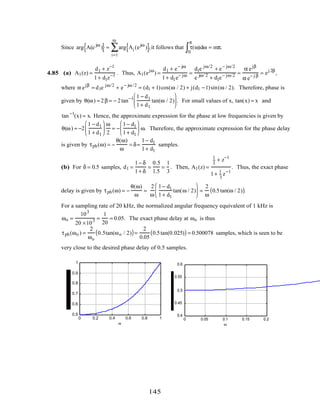
150. 4.86 A2(e jω
) =
d2 + d1e−jω
+ e−j2ω
1 + d1e−jω
+ d2 e−j2ω =
d2 ejω
+ d1 + e−jω
ejω
+ d1 + d2 e−jω
=
(d1 + d2 cosω + cosω) + j(d2 sinω − sinω)
(d1 + d2 cosω + cosω) + j(sinω − d2 sinω)
=
d1 + (d2 +1)cosω( ) + j(d2 − 1)sin ω
d1 + (d2 +1)cosω( ) − j(d2 − 1)sin ω
. Therefore
θ(ω) = 2tan−1 (d2 − 1)sin ω
d1 + (d2 + 1)cosω





 . Now, τp (ω) = −
θ(ω)
ω
= −
2
ω
tan−1 (d2 − 1)sinω
d1 + (d2 +1)cosω





 .
For ω ≅ 0, sinω = ω and cosω = 1. Then τp (ω) = −
2
ω
tan−1 (d2 − 1)ω
d1 + (d2 + 1)





 . Again, for x ≅ 0,
tan−1
x ≅ x. Hence, τp (ω) = −
2
ω
(d2 −1)ω
d1 + (d2 + 1)
= −
2(d2 − 1)
d1 + d2 + 1
= δ.
Now, substituting d1 = 2
2 − δ
1+ δ





 and d2 =
(2 − δ)(1− δ)
(2 + δ)(1+ δ)
we can show easily that
−
2(d2 − 1)
d1 + d2 +1
= δ.
4.87 Since G(z) is non-minimum phase but causal, it will have some zeros outside the unit circle. Let
z = α be one such zero. We can then write G(z) = P(z)(1–αz
−1
) = P(z)(−α* +z
−1
)
1−αz
−1
−α *+z
−1







 ,
Note that
1− αz
−1
−α*
+ z−1





 is a stable first order allpass function. If we carry out this operation for
all zeros of G(z) that are outside the unit circle we can write G(z) = H(z)A(z) where H(z) will
have all zeros inside the unit circle and will thus be a minimum phase function and A(z) will be
a product of first order allpass functions, and hence an allpass function.
4.88 H(z) =
(z +1.4)(z2
+ 2z + 4)
(z + 0.8)(z − 0.6)
. In order to correct for magnitude distortion we require the
transfer function G(z) to satisfy the following property G(e
jω
) =
1
H(e
jω
)
. Hence, one possible
solution is Gd(z) =
1
H(z)
=
(z + 0.8)(z − 0.6)
(z +1.4)(z2 + 2z + 4)
. Since Gd(z) has poles outside the unit circle.
it is not stable. Therefore we require a stable transfer function with magnitude response same as
Gd(z). Using the technique of the previous problem we thus get:
G(z) =
(z + 0.8)(z − 0.6)
(z +1.4)(z2 + 2z + 4)
(z2
+ 2z + 4)
(4z2 + 2z +1)
(z +1.4)
(1.4z + 1)
=
(z + 0.8)(z − 0.6)
(4z2 + 2z +1)(1.4z + 1)
is the desired stable
solution such that G(ejω
) H(ejω
) = 1.
4.89 (a) G(z) = H(z) A(z) where A(z) is an allpass function. Then, g[0] = lim
z→∞
G(z).
g[0] = lim
z→∞
G(z) = lim
z→∞
H(z)A(z) = lim
z→∞
H(z)A(z) = lim
z→∞
H(z) lim
z→∞
A(z)
146

151. ≤ lim
z→∞
H(z) because lim
z→∞
A(z) < 1 (see Problem 4.71)
≤ h[0]
(b) If λl is a zero of H(z), then λl <1, since H(z) is a minimum-phase causal stable transfer
function which has all zeros inside the unit circle. We can express H(z) = B(z)(1− λl z−1
). It
follows that B(z) is also a minimum-phase causal transfer function.
Now consider the transfer function F(z) = B(z)(λl
*
− z−1
) = H(z)
(λl
* − z−1)
(1− λl
z−1)
. If h[n], b[n], and
f[n] denote, respectively, the inverse z-transforms of H(z), B(z), and F(z), then we get
h[n] =
b[0], n = 0
b[n] − λl b[n −1], n ≥ 1,



and f[n]=
λl
*
b[0], n = 0,
λl
*
b[n]− b[n −1], n ≥1.




Consider ε = h[n]
2
n=0
m
∑ − f[n]
2
n=0
m
∑ = b[0]
2
− λl
* 2
b[0]
2
+ h[n]
2
n =1
m
∑ − f[n]
2
n =1
m
∑ .
Now h[n]
2
= b[n]
2
+ λl
2
b[n −1]
2
− λl b[n−1]b*[n]− λl
*
b*[n −1]b[n], and
f[n]
2
= λl
2
b[n]
2
+ b[n −1]
2
− λl b[n −1]b*[n]− λl
*
b*[n −1]b[n],
Hence, ε = b[0]
2
− λl
2
b[0]
2
+ b[n]
2
+ λl
2
b[n −1]
2





n=1
m
∑ − λl
2
b[n]
2
− b[n −1]
2





n =1
m
∑
= 1− λl
2




 b[m]
2
.
Since λl <1, ε > 0, i.e, h[n]
2
n =0
m
∑ > f[n]
2
n=0
m
∑ . Hence, h[n]
2
n =0
m
∑ ≥ g[n]
2
n=0
m
∑ .
4.90 H(z) =
(z + 3)(z − 2)
(z − 0.25)(z + 0.5)
= G(z)A(z) =
(3z+ 1)(1 − 2z)
(z− 0.25)(z + 0.5)
(z + 3)(z− 2)
(3z +1)(1 − 2z)
Therefore G(z) =
(3z + 1)(1 − 2z)
(z− 0.25)(z + 0.5)
. The inverse z-transforms of these causal transfer
functions are given by h[n] ={1, 0.75, −6.0625, 1.6093, –1.16015, L}, and
g[n]= {− 6, 2.5, – 0.375, 0.40625, –0.1484, 0.0879, L}, respectively. It can be
seen that g[n]
2
n=0
m
∑ is bigger than h[n]
2
n=0
m
∑ for all values of m.
4.91 See Example 4.13.
(a) HBS(z) =
1
4
(1+ z
−2
)
2
. Thus, HBP(z) = z
−2
−
1
4
(1+ z
−2
)
2
= −
1
4
(1− z
−2
)
2
.
(b) HBS(z) =
1
16
(1+ z
−2
)(−1+ 6z
−2
− z
−4
). Thus, HBP(z) = z
−4
−
1
16
(1+ z
−2
)(−1+ 6z
−2
− z
−4
)
147

152. =
1
16
1− 4z
−2
+ 6z
−4
− 4z
−6
+ z
−8
{ } =
1
16
(1− z
−2
)
4
.
(c) HBS(z) =
1
32
(1+ z
−2
)
2
(−3+14z
−2
− 3z
−4
). Thus,
HBP(z) = z
−4
−
1
32
(1+ z
−2
)
2
(−3 +14z
−2
− 3z
−4
) =
1
32
3−8z
−2
+10z
−4
− 8z
−6
+ 3z
−8
{ }
=
1
32
3−8z
−2
+10z
−4
− 8z
−6
+ 3z
−8
{ }.
4.92 H0(z) = A0 (z)+ A1(z), and H1(z) = A0(z) – A1(z),where A0(z) and A1(z) are allpass
functions of orders M and N, respectively, with no common factors. Hence, the orders of H0(z)
and H1(z) are M+N. Now, we can write A0(z) =
z
– M
D0 (z
–1
)
D0(z)
, and A1(z) =
z–ND1(z–1)
D1(z)
.
Then, H0(z) =
P(z)
D(z)
=
z
−M
D0(z
−1
)D1(z)+ z
−N
D0(z)D1(z
−1
)
D0(z)D1(z)
, and
H1(z) =
Q(z)
D(z)
=
z
−M
D0 (z
−1
)D1(z) – z
−N
D0 (z)D1(z
−1
)
D0 (z)D1(z)
.
Since P(z) is of degree M+N and z
–(M+N)
P(z
–1
) = z
–(M+N)
z
M
D0(z)D1(z
–1
) + z
N
D0 (z
–1
)D1(z)( )
= z
–N
D0 (z)D1(z
–1
) + z
–M
D0(z
–1
)D1(z) = P(z). Hence P(z) is symmetric. Similarly one can
prove that Q(z) is anti-symmetric.
4.93 H0(z) =
1
2
A0 (z) + A1(z)[ ], H1(z) =
1
2
A0(z) –A1(z)[ ]. Thus, H0(z)H0 (z
–1
) + H1(z)H1(z
–1
)
=
1
4
A0(z) + A1(z)[ ] A0 (z
–1
)+ A1(z
–1
)[ ]+
1
4
A0(z) – A1(z)[ ] A0 (z
–1
)– A1(z
–1
)[ ].
=
1
4
A0(z)A0 (z
–1
)+ A0(z)A1(z
–1
) + A1(z)A0 (z
–1
)+ A1(z)A1(z
–1
)[ ]
+
1
4
A0(z)A0 (z
–1
) – A0(z)A1(z
–1
)– A1(z)A0(z
–1
)+ A1(z)A1(z
–1
)[ ]
=
1
2
A0(z)A0(z
–1
) + A1(z)A1(z
–1
)[ ]= 1. Thus, H0(e
jω
)
2
+ H1(e
jω
)
2
= 1 implying that
H0 (z) and H1(z) form a power complementary pair.
4.94 H0(e
jω
)
2
=
1
4
A0 (e
jω
)A0
*
(e
jω
) + A1(e
jω
)A0
*
(e
jω
)+ A0 (e
jω
)A1
*
(e
jω
) + A1(e
jω
)A1
*
(e
jω
){ }.
Since A0(z) and A1(z) are allpass functions, A0(e
jω
) = e
jφ0(ω)
and A1(e
jω
) = e
jφ1(ω)
.
Therefore H0(e
jω
)
2
=
1
4
2 + e
j(φ0(ω)−φ1(ω))
+ e
−j(φ0 (ω)−φ1(ω))
{ }≤1 as maximum values of
e
j(φ0(ω)−φ1(ω))
and e
−j(φ0 (ω)−φ1(ω))
are 1. H0(z) is stable since A0(z) and A1(z) are stable
transfer functions. Hence, H0(z) is BR.
148

153. 4.95 H(z) =
1
M
Ak (z)
k=0
M−1
∑ . Thus, H(z)H(z
−1
) =
1
M
2 Ak (z)
k=0
M−1
∑
r=0
M−1
∑ Ar(z
−1
). Hence,
H(e
jω
)
2
=
1
M
2 e
j(φk (ω)−φr(ω))
k=0
M−1
∑
r=0
M−1
∑ ≤1. Again H(z) is stable since {Ai(z)} are stable
transfer functions. Hence, H(z) is BR.
4.96 HBP(z) =
1− α
2
1− z
−2
1− β(1+ α)z
−1
+ αz
−2







 and HBS(z) =
1− α
2
1− 2βz
−1
+ z
−2
1− β(1+ α)z
−1
+ αz
−2 .
HBS(z) + HBP(z) =
1− α − z
−2
+ αz
−2
+ 1− 2βz
−1
+ z
−2
+ α − 2αβz
−1
+ αz
−2
2(1− β(1+ α)z
−1
+ αz
−2 = 1.
Hence HBP(z) and HBS(z) are allpass complementary.
4.97 H(z)H(z−1
)+ H(−z)H(−z−1
) = K. On the unit circle, this reduces to
H(ejω
)H(e− jω
)+ H(−ejω
)H(−e− jω
) = K, or equivalently, H(ejω
)
2
+ H(−e jω
)
2
= K, as H(z) is a
real-coefficient transfer function. Now, H(−ejω
)
2
= H(e j(π+ω)
)
2
. Hence, for ω = π / 2, the
power-symmetric condition reduces to
H(ejπ/ 2
)
2
+ H(e j(π+π / 2)
)
2
= H(ejπ/ 2
)
2
+ H(ej(2π−π/ 2)
)
2
= K. Since H(z) is a real-coefficient
transfer function, H(ejω
)
2
is an even function of ω , and thus, H(ejπ/ 2
)
2
= H(e j(2π−π/ 2)
)
2
.
As a result, 2H(ejπ / 2
)
2
= K, from which we obtain 10 log10 2 + 20log10 H(ejπ/ 2
) =10 log10 K,
or 20 log10 H(ejπ/ 2
) = G(ω)ω=π/ 2
= 10log10 K − 3.
4.98 H(z) = A0 (z2
) +−1
A1(z2
). Therefore,
H(z)H(z−1
) + H(−z)H(−z−1
) = A0(z2
)+ z−1
A1(z2
)[ ]A0(z−2
) + zA1(z−2
)[ ]
+ A0 (−z)2
( )− z−1
A1 (−z)2
( )[ ]A0 (−z)2
( )− zA1 (−z)2
( )[ ]
= A0(z2
)A0 (z−2
) + z−1
A1(z2
)A0 (z−2
)+ z A0 (z2
)A1(z−2
) + A1(z2
)A1(z−2
)
+ A0(z2
)A0 (z−2
) − z−1
A1(z2
)A0 (z−2
)− z A0 (z2
)A1(z−2
) + A1(z2
)A1(z−2
) = 4, as
A0(z2
)A0 (z−2
) = A1(z2
)A1(z−2
) = 1.
4.99 (a) Ha(z) =
1
2
− z−1
+
21
2
z−2
−
27
2
z−3
− 5z−4
−
5
2
z−5
. Thus,
Ha(z)Ha (z−1
) = −1.25z5
− 28z3
− 72,75z + 325− 72,75z−1
− 28 z−3
−1.25z−5
and
Ha(−z)Ha(−z−1
) = 1.25z5
+ 28z3
+ 72,75z + 325 + 72,75z−1
+ 28z−3
+ 1.25z−5
. Hence,
Ha(z)Ha (z−1
) + Ha (−z)Ha (−z−1
) = 650.
149

154. (b) Hb (z) =1 + 3z−1
+ 14z−2
+ 22z−3
− 12z−4
+ 4z−5
. Thus,
Hb (z)Hb (z−1
) = 4z5
+ 42z3
+ 41z + 850 + 41z−1
+ 42z−3
+ 4z−5
and
Hb (−z)Hb(−z−1
) = −4z5
− 42 z3
− 41z + 850 − 41z−1
− 42z−3
− 4z−5
. Hence,
Hb (z)Hb (z−1
) + Hb(−z)Hb (−z−1
) = 1700.
4.100 H(z)H(z−1
) = a2
(1+ bz−1
)(1+ bz) = a2
bz + a2
(1+ b2
) + a2
bz−1
. Thus, c = a2
b and
d = a2
(1+ b2
). Now, H(z)H(z−1
) + H(−z)H(−z−1
) = cz + d + c z−1
− cz + d − c z−1
= 2d. Therefore,
2d = 2a2
(1+ b2
) = 1. This condition is satisfied by a = 1/ 2(1+ b2
) . For b = 1, then a =
1
2
.
Other solutions include b = –1 and a =
1
2
, b = 2 and a =
1
10
.
Since H(z) is a first-order FIR causal FIR transfer function, G(z) = − z−1
H(−z−1
) is also a first-
order FIR causal FIR transfer function. Now,
H(z)H(z−1
) + G(z)G(z−1
) = H(z)H(z−1
) + − z−1
H(− z−1
)[ ]− zH(−z)[ ]
= H(z)H(z−1
) + H(−z)H(−z−1
) = 1. Hence H(z) and G(z) are power-complementary.
4.101 H(z)H(z−1
) = (c z + d + cz−1
) d2z2
+ d1(1+ d2 )z + (1 + d1
2
+ d2
2
) + d1(1+ d2 )z−1
+ d2z−2
[ ].
Thus, H(z)H(z−1
) + H(−z)H(−z−1
) = 2[cd1(1+ d2 )z2
+ 2c d1(1+ d2 ) + dd2z2
+ d(1+ d1
2
+ d2
2
)
+dd2z−2
+ c d1(1+ d2 )z−2
] = 1. Hence, we require
dd2 + c d1(1+ d2 )= 0, and 2cd1(1+ d2) + d(1+ d1
2
+ d2
2
) =1. Solving these two equations we
arrive at c =
d2
d2 (1+ d2 )(2d2 −1− d1
2
− d2
2
)
and d = −
1
2d2 − 1− d1
2
− d2
2 . For d1 = d2 = 1, we get
c = −
1
2
and d = 1.
Since H(z) is a third-order FIR causal FIR transfer function, G(z) = − z−3
H(− z−1
) is also a third-
order FIR causal FIR transfer function. Now,
H(z)H(z−1
) + G(z)G(z−1
) = H(z)H(z−1
) + − z−3
H(− z−1
)[ ] −z3
H(− z)[ ]
= H(z)H(z−1
) + H(−z)H(−z−1
) = 1. Hence H(z) and G(z) are power-complementary.
4.102 H(z) =
0.1 + 0.5z−1
+ 0.45z−2
+ 0.45z−3
+ 0.5z−4
+ 0.1z−5
1+ 0.9z−2
+ 0.2z−4 =
1
2
A(z2
) + z−1
[ ], where
A(z) =
0.2 + 0.9z−1
+ z−2
1+ 0.9z−1
+ 0.2z−2 is a stable allpass function. Thus,
H(z)H(z−1
) + H(−z)H(−z−1
) =
1
4
A(z2
) + z−1
[ ] A(z−2
) + z[ ]+
1
4
A(z2
) − z−1
[ ]A(z−2
) − z[ ]= 1.
4.103 (a) H1(z) =
1
1+ α
(1+ αz
−1
).
150

155. H1(e
jω
)
2
=
1
(1+ α)
2 (1+ αcosω)
2
+ (αsinω)
2
{ } =
1+ α
2
+ 2αcosω
(1+ α)
2 . Thus,
dH1
(ejω
)
2
dω
=
–2αsinω
(1+ α)
2 < 0, for a > 0. The maximum value of H1(e
jω
) = 1 at w = 0, and the
minimum value is at w = π. On the other hand, if a < 0, then
dH1
(ejω
)
2
dω
> 0, In this case the
maximum value of H1(e
jω
) = (1–α)
2
/(1+ α)
2
> 1 at w = π, and the minimum value is at w =
0. Hence, H1(z) is BR only for a > 0.
(b) H2(z) =
1
1+ β
(1−βz
−1
). H2(e
jω
)
2
=
1+ β
2
− 2βcosω
(1+ β)
2 . Thus,
dH2
(ejω
)
2
dω
=
2βsinω
(1+ β)
2 > 0, for b > 0. The maximum value of H2(e
jω
) = 1 at w = π, and the
minimum value is at w = 0. On the other hand, if b < 0, then
dH2
(ejω
)
2
dω
< 0, In this case the
maximum value of H2(e
jω
) = (1–β)
2
/(1+ β)
2
> 1 at w = 0, and the minimum value is at w =
π. Hence, H2(z) is BR only for b > 0.
(c) H3(z) =
(1+ αz
−1
)(1–βz
−1
)
(1+ α)(1+ β)
. From the results of Parts (a) and (b) it follows that H3(z) is BR
only for a > 0 and b > 0.
(d) H4(z) =
(1+ 0.4z
−1
)(1+ 0.5z
−1
)(1+ 0.6z
−1
)
3.36
=
1+ 0.4z
−1
1.4








1+ 0.5z
−1
1.5








1+ 0.6z
−1
1.6







 . Since
each individual factors on the right-hand side is BR, H4(z) is BR.
4.104 (a) H1(z) =
2 + 2z
–1
3+ z
–1 =
1
2
1+
1+ 3z
–1
3+ z
–1







 =
1
2
A0 (z) + A1(z)( ), where A0(z) = 1 and
A1(z) =
1+ 3z
–1
3+ z
–1 are stable allpass functions. In view of Problem 4.80, H1(z) is BR.
(b) H2(z) =
1– z
–1
4+ 2z
–1 =
1
2
1–
2 + 4 z
–1
4 + 2z
–1







 =
1
2
A0 (z) – A1(z)( ), where A0(z) = 1 and
A1(z) =
2 + 4 z
–1
4 + 2z
–1 are stable allpass functions. In view of Problem 4.79, H1(z) is BR.
151

156. (c) H3(z) =
1–z
–2
4 + 2z
–1
+ 2z
–2 =
1
2
1–
2 + 2z
–1
+ 4z
–2
4+ 2z
–1
+ 2z
–2







 , where A1(z) =
2 + 2z
–1
+ 4z
–2
4 + 2z
–1
+ 2z
–2 is a
stable allpass function. Hence, H3(z) is BR.
(d) H4(z) =
3 + 6z
–1
+ 3z
–2
6+ 5z
–1
+ z
–2 =
1
2
1+
1+ 3z
–1
3+ z
–1
















1
2
1+
1+ 2z
–1
2 + z
–1
















which is seen to be a product
of two BR functions. Hence, H4(z) is BR.
(e) H5(z) =
3 + 2z
–1
+ 3z
–2
4 + 2z
–1
+ 2z
–2 =
1
2
1+
2 + 2z
–1
+ 4z
–2
4+ 2z
–1
+2z
–2







 =
1
2
1+ A1(z)( ) where
A1(z) =
2 + 2z
–1
+ 4z
–2
4+ 2z
–1
+ 2z
–2 is a stable allpass funcion. Hence, H5(z) is BR.
(f) H6(z) =
3+ 9z
–1
+ 9z
–2
+ 3z
–3
12 + 10z
–1
+ 2z
–2 =
1
2
1+
1+ 3z
–1
3+ z
–1
















1
2
1+
1+ 2z
–1
2 + z
–1
















1+ z
–1
2







 which is seen
to be a product of three BR functions. Hence, H6(z) is BR.
4.105 Since A1(z) and A2(z) are LBR, aa A1(e
jω
) = 1 and A2(e
jω
) =1. Thus, A1(e
jω
) = e
jφ1(ω)
,
and A2(e
jω
) = e
jφ2(ω)
. Now, A1
1
A2(e
jω
)







 = A1 e
–jφ2 (ω)
( ). Thus, A1(e
−jφ2(ω)
) = 1. Hence,
A1
1
A2(z)







 is LBR.
4.106 F(z) = z
G(z) + α
1+ αG(z)





 . Thus, F(e
jω
) = e
jω G(e
jω
)+ α
1+ αG(e
jω
)







 = e
jω e
jφ(ω)
+ α
1+ αe
jφ(ω)







 since G(z) is LBR.
F(e
jω
)
2
=
e
jφ(ω)
+ α
1+ αe
jφ(ω)
2
=
cosφ(ω) + α( )
2
+ sinφ(ω)( )
2
1+ αcosφ(ω)( )2
+ α sinφ(ω)( )2 =
1+ 2α cosφ(ω)+ α
2
1+ 2α cosφ(ω)+ α
2 = 1.
Let z = l be a pole of F(z). This implies, G(l) = – 1/a or G(λ) = 1/ α. If α < 1, then
G(λ) > 1, which is satisfied by the LBR G(z) if λ < 1. Hence, F(z) is LBR. The order of F(z) is
same as that of G(z).
G(z) can be realized in the form of a two-pair constrained by the transfer function F(z).
152

157. To this end, we express G(z) in terms of F(z) arriving at G(z) =
–α + z
–1
F(z)
1–αz
–1
F(z)
=
C + DF(z)
A + BF(z)
,
where A, B, C, and D, are the chain parameters of the two-pair. Comparing the two expressions
on the right-hand side we get A = 1, B = –αz
–1
, C = –α, and D = z
–1
. The corresponding
transfer parameters are given by t11 = –α, t21 = 1, t12 = (1– α
2
)z
–1
, and t22 = α z
–1
.
4.107 Let F(z) = G
1
A(z)





 . Now A(z) being LBR, A(e
jω
) = e
jφ(ω)
. Thus,
F(ejω
) = G
1
A(ejω)





 = G(e−jφ(ω)
). Since G(z) is a BR function, G(e
−jφ(ω)
) ≤ 1. Hence,
F(ejω
) = G
1
A(ejω )





 ≤1.
Let z = ξ be a pole of F(z). Hence, F(z) will be a BR function if |ξ| < 1. Let z = λ be a pole
of G(z). Then this pole is mapped to the location z = ξ of F(z) by the relation
1
A(z) z=ξ
= λ, or A(ξ) =
1
λ
. Hence, A(ξ) =
1
λ
>1 because of Eq. (4.129). This implies,
λ < 1. Thus G
1
A(z)





 is a BR function.
4.108 (a) H(z) =
2+ 2z
−1
3 + z
−1 , G(z) =
1− z
−1
3+ z
−1 . Now, H(z)+ G(z) =
2+ 2z
−1
3+ z
−1 +
1− z
−1
3 + z
−1 =
3+ z
−1
3+ z
−1 = 1.
Next, H(z)H(z
−1
) + G(z)G(z
−1
) =
2 + 2z
−1
3+ z
−1
2 + 2z
3+ z
+
1− z
−1
3+ z
−1
1+ z
3+ z
=
4 + 4z
−1
+ 4z + 4 +1+1− z
−1
− z
(3+ z
−1
)(3+ z)
= 1. Thus, H(e
jω
)
2
+ G(e
jω
)
2
= 1
Hence H(z) and G(z) are both allpass-complementary and power complementary. As a result,
they are doubly complementary.
(b) H(z) =
−1+ z
−2
4 + 2z
−1
+ 2z
−2 , G(z) =
3+ 2z
−1
+ 3z
−2
4 + 2z
−1
+ 2z
−2 . Note H(z) + G(z) =
2 + 2z
−1
+ 4z
−2
4 + 2z
−1
+ 2z
−2
implying that H(z) and G(z) are allpass complementary. Next, H(z)H(z
−1
) + G(z)G(z
−1
)
=
−1+ z
−2
4 + 2z
−1
+ 2z
−2
−1+ z
2
4 + 2z + 2z
2 +
3+ 2z
−1
+ 3z
−2
4+ 2z
−1
+ 2z
−2
3+ 2z + 3z
2
4+ 2z + 2z
2
=
1+1− z
−2
− z
2
+ 9 + 6z + 9z
2
+ 6z
−1
+ 4 + 6z + 9z
−2
+ 6z
−1
+ 9
(4 + 2z
−1
+ 2z
−2
)(4 + 2z + 2z
2
)
= 1. Hence, H(z)
and G(z) are also power complementary. As a result, they are doubly-complementary.
153

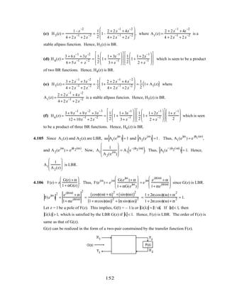
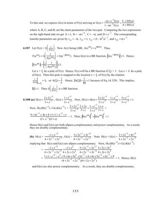
158. 4.109 (a) Ha(z) =
2(1+ z
–1
+z
–2
)
3+ 2z
–1
+ z
–2 =
1
2
1+
1+ 2z
–1
+ 3z
–2
3 + 2z
–1
+ z
–2







 . Its power-complementary transfer
function therefore is given by Ga(z) =
1
2
1–
1+ 2z
–1
+ 3z
–2
3 + 2z
–1
+ z
–2







 =
1– z
–2
3+ 2z
–1
+ z
–2 .
(b) Hb(z) =
3(1.5 + 6.5z−1
+ 6.5z−2
+1.5z−3
)
18 + 21z−1 +8z−2 + z−3 =
3(1.5+ 6.5z−1
+ 6.5z−2
+1.5z−3
)
(2 +z−1)(3+ z−1)(3+ z−1)
=
1
2
(1+2z−1
)(1+ 3z−1
)
(2+ z−1)(3 +z−1)
+
1+3z−1
3+ z−1








. Its power-complementary transfer
function therefore is given by
Gb(z) =
1
2
(1+ 2z−1
)(1+ 3z−1
)
(2 + z−1)(3+ z−1)
−
1+ 3z−1
3+ z−1








=
−1.5 −3.5z−1
+ 3.5z−2
+1.5z−3
18 + 21z−1 + 8z−2 + z−3 .
4.110 G0(e
jω
)
2
+ G1(e
jω
)
2
=
1
4
A0(e
jω
)+ A1(e
jω
)
2
+ A0(e
jω
) − A1(e
jω
)
2





=
1
4
A0(ejω
) + A1(ejω
)( ) A0
*
(ejω
)+ A1
*
(e jω
)( )+ A0(ejω
)− A1(ejω
)( ) A0
*
(ejω
) − A1
*
(ejω
)( ){ }
=
1
4
{A0 (ejω
)A0
*
(ejω
) + A1(ejω
)A1
*
(ejω
) + A0 (ejω
)A1
*
(e jω
)+ A1(ejω
)A0
*
(ejω
)
+ A0(ejω
)A0
*
(ejω
)+ A1(ejω
)A1
*
(e jω
)− A0(ejω
)A1
*
(ejω
)− A1(ejω
)A0
*
(e jω
)}
=
1
4
2A0(e
jω
)
2
+ 2A1(e
jω
)
2





= 1.
4.111 Let the output of the predictor in Figure P4.11(a) be denoted by E(z). Then analyzing this
figure we get E(z) = P(z)[U(z) + E(z)] and U(z) = X(z) − E(z). From the first equation we
have E(z) =
P(z)
1− P(z)
U(z) which when substituted in the second equation yields
H(z) =
U(z)
X(z)
= 1− P(z).
Analyzing Figure P4.11(b) we arrive at Y(z) = V(z) + P(z)Y(z) which yields
G(z) =
Y(z)
V(z)
=
1
1− P(z)
, which is seen to be the inverse of H(z).
For P(z) = h1z−1
, H(z) = 1− h1z−1
and G(z) =
1
1− h1z−1 . Similarly, for P(z) = h1z−1
+ h2z−2
,
H(z) = 1− h1z−1
− h2z−2
and G(z) =
1
1− h1z−1
− h2z−2 .
4.112 The z-transform of h1[n] is given by H1(z) =
5 / 3
1− 0.5z−1 +
1 / 12
1+ 0.2z−1 − 1. Using the M-file
residuez we arrive at H1(z) =
0.75 + 0.5917z−1
+ 0.1z−2
1− 0.3z−1
− 0.1z−2 =
0.75(1+ 0.5436 z−1
)(1+ 0.2453z−1
)
(1− 0.5z−1
)(1+ 0.2z−1
)
.
154

159. Since the zeros of the numerator of H1(z) are inside the unit circle, the inverse system is causal
and stable. Hence, the transfer function of the inverse system is given by
H2(z) =
1− 0.3z−1
− 0.1z−2
0.75 + 0.5917z−1 + 0.1z−2 =
1.3333− 0.4z−1
− 0.1333z−2
1+ 0.7889z−1 + 0.1333z−2 A partial-fraction expansion of
H2(z) using the M-file residuez yields H2(z) =
2.9474
1+ 0.5437z−1 −
0.6141
1+ 0.2452z−1 − 1 whose inverse
z-transform is given by H2(z) = 2.9474(−0.5437)n
µ[n]− 0.6141(−0.2452)n
µ[n]− δ[n].
4.113 X1 = A Y2 + BX2, Y1 = CY2 + D X2 . From the first equation, Y2 =
1
A
X1 –
B
A
X2.
Substituting this in the second equation we get
Y1 = C
1
A
X1 –
B
A
X2





 + DX2 =
C
A
X1 +
AD –BC
A
X2, Comparing the last two equations with
Eq. (4.146) we arrive at t11 =
C
A
, t12 =
AD – BC
A
, t21 =
1
A
, t22 = –
B
A
.
Next, Y1 = t22X1 + t12X2, Y2 = t21X1 + t22X2. From the second equation we get
X1 = –
t22
t21
X2 +
1
t21
Y2. Substituting this expression in the first equation we get,
Y1 = t11 –
t22
t21
X2 +
1
t21
Y2







 + t12X2 =
t11
t21
Y2 +
t12t21 – t11t22
t21
X2. Comparing the last two
equations with Eq. (4.149) we arrive at A =
1
t21
, B = –
t22
t21
, C =
t11
t21
, D =
t12t21 – t11t22
t21
.
4.114 From Eq. (4.176a) we note t12 =
AD − BC
A
and t21 =
1
A
. Hence, t12 = t21 imply
A D − BC = 1.
4.115
Y1
'
Y2
'








=
k1 (1− k1
2
)z
−1
1 −k1z
−1








X1
'
X2
'








,
Y1
"
Y2
"








=
k2 (1− k2
2
)z
−1
1 −k2z
−1








X1
"
X2
"








, where
X1
"
X2
"








=
Y1
'
Y2
'








.
Thus, the transfer matrices of the two two-pairs are given by τ1 =
k1 (1− k1
2
)z−1
1 −k1z−1








, and
τ2 =
k2 (1− k2
2
)z−1
1 −k2z−1








. The corresponding chain matrices are obtained using Eq. (4.76b) and
are given by Γ1 =
1 k1z–1
k1 z–1








, and Γ2 =
1 k2z–1
k2 z–1








. Therefore, the chain matrix of the Γ -
cascade is given by Γ1Γ2 =
1 k1z–1
k1 z–1








1 k2z–1
k2 z–1








=
1+ k1k2z−1
k2z−1
+ k1z−2
k1 + k2z−1
k1k2z−1
+ z−2








.
Hence using Eq. (4.176a) we arrive at the transfer matrix of the Γ -cascade as
155

160. τ =
k1
+ k2
z−1
1+ k1k2z−1
z−2(1− k1
2 )(1− k1
2)
1+ k1k2z−1
1
1+ k1
k2
z−1
−
z−1
(k2 + k1z−1
)
1+ k1
k2
z−1
















.
4.116
X1
'
Y1
'








=
1 k1z
–1
k1 z
–1








Y2
'
X2
'








,
X1
"
Y1
"








=
1 k2z
–1
k2 z
–1








Y2
"
X2
"








, where
Y2
'
X2
'








=
X1
"
Y1
"








. Therefore,
the chain matrices of the two two-pairs are given by Γ1 =
1 k1z–1
k1 z–1








, and Γ2 =
1 k2z–1
k2 z–1








.
The corresponding transfer matrices are obtained using Eq. (4.151a) and are given by
τ1 =
k1 (1− k1
2
)z−1
1 −k1z−1








, and τ2 =
k2 (1− k2
2
)z−1
1 −k2z−1








. The transfer matrix of the t-cascade is
therefore given by τ = τ2τ1 =
k2 (1− k2
2
)z−1
1 −k2z−1








k1 (1− k1
2
)z−1
1 −k1z−1








=
k1k2 + z−1
(1− k2
2
) z−1
k2(1− k1
2
) − z−2
k1(1− k2
2
)
k1 − k2z−1
z−1
(1− k1
2
)+ k1k2z−2








.
Using Eq. (4.151b) we thus arrive at the chain matrix of the t-cascade:
Γ =
1
k1 − k2z−1
−(k1
k2
z−1 +1− k1
2)z−1
k1 − k2z−1
k1k2 + z−1
(1− k2
2
)
k1
− k2
z−1
z−2
k1
− k2
z−1
















.
4.117 (a) Analyzing Figure P4.13(a) we obtain Y2 = X1 − kmz−1
X2 and Y1 = kmY2 + z−1
X2
= km X1 − kmz−1
X2( )+ z−1
X2 = kmX1 + 1− km
2
( )z−1
X2 . Hence, the transfer parameters are given
by τ =
km (1− km
2
)z−1
1 −kmz−1








. Using Eq. (4.176b) we arrive at the chain parameters given by
Γ =
1 kmz−1
km z−1








.
(b) Analyzing Figure P4.13(a) we obtain V1 = km X1 − z−1
X2( ) ,
Y1 = V1 + X1 = (1+ km )X1 − kmz−1
X2, and Y2 = V1 + z−1
X2 = kmX1 + (1− km)z−1
X2. Hence, the
transfer parameters are given by τ =
1+ km −kmz−1
km (1− km)z−1








. Using Eq. (4.176b) we arrive at the
chain parameters given by Γ =
1
km
−
(1 − k
m
)z−1
km
1− k
m
km
−
1
km














.
156

161. 4.118 For the constrained two pair H(z) =
C + DG(z)
A + BG(z)
. Hence, C = km, D = z
–1
, A = 1, B= kmz
−1
.
Substituting these values of the chain parameters in Eq. (4.151a) we get
t11 =
C
A
= km, t12 = z
−1
(1− km
2
), t21 = 1, t22 = −kmz
−1
.
4.119 From the results of Problem 4.117, Part (a), we observe that the chain matrix of the i-th lattice
two-pair is given by Γi =
1 kiz−1
ki z−1








, i = 1,2,3. Thus, the chain matrix of the cascade of three
lattice two-pairs is given by Γcascade =
1 k1z−1
k1 z−1








1 k2z−1
k2 z−1








1 k3
z−1
k3 z−1








=
1 k1z−1
k1 z−1








1+ k2
k3
z−1 k3
z−1 + k2
z−2
k2 + k3z−1
k2k3z−1
+ z−2








=
1+ k2
k3
z−1 + k1
z−1(k2
+ k3
z−1) k3
z−1 + k2
z−2 + k1
z−1(k2
k3
+ z−2 )
k1(1+ k2k3z−1
)+ z−1
(k2 + k3z−1
) k1(k3z−1
+ k2z−2
)+ z−1
(k2k3 + z−2
)








. From Eq. (4.181a)
we obtain A3(z) =
C + D
A + B
=
1+ k2k3z−1 + k1z−1(k2 + k3z−1) + k3z−1 + k2z−2 + k1z−1(k2k3 + z−2 )
k1
(1+ k2
k3
z−1) + z−1(k2
+ k3
z−1) + k1
(k3
z−1 + k2
z−2) + z−1(k2
k3
+ z−2)
=
k1 + (k2k3 + k1k2 + k3)z−1 + (k1k3 + k2 + k1k2k3 )z−2 + k1z−3
k1
+ (k1
k3
+ k2
+ k1
k2
k3
)z−1 + (k2
k3
+ k1
k2
+ k3
)z−2 + z−3 which is seen to be an allpass
function.
4.120 Let D(z) =1+ d1z−1
+ d2z−2
= (1− λ1z−1
)(1− λ2z−1
). Thus, d2 = λ1λ2 and d1 = –(λ1 + λ2 ).
For stability, λi < 1, i = 1, 2. As a result, d2 = λ1λ2 <1.
Case 1: Complex poles: d2 > 0. In this case, λ2 = λ1
*
. Now,
λ1,λ2 =
−d1 ± d1
2 − 4d2
2
. Hence, λ1 and λ2 will be complex, if d1
2
< 4d2. In this case,
λ1 = –
d1
2
+
j
2
4d2 − d1
2
. Thus, λ1
2
=
1
4
d1
2
+ 4d2 − d1
2
( )= d2 < 1. Consequently, if the poles
are complex and d2 < 1, then they are inside the unit circle.
Case 2: Real poles. In this case we get –1< λi < 1, i = 1, 2. Since, λi < 1, it follows then
d1 < λ1 + λ2 < 2. Now, −1<
− d1 ± d1
2 − 4d2
2
<1, or ± d1
2
− 4d2 < 2 + d1.
It is not possible to satisfy the inequality on the right hand side with a minus sign in front of
the square root as it would imply then d1 < – 2. Therefore,
d1
2
− 4d2 < 2 + d1, or d1
2
− 4d2 < 4+ d1
2
+ 4d1, or –d1 <1+ d2. (14)
157

162. Similarly,
− d1 ± d1
2 − 4d2
2
< −1, or ± d1
2
− 4d2 > –2 + d1. Again it is not possible to
satisfy the inequality on the right hand side with a plus sign in front of the square root as it
would imply then d1 > 2. Therefore, − d1
2
− 4d2 > –2 + d1, or d1
2
− 4d2 <2 − d1,or
d1
2
− 4d2 < 4+ d1
2
− 4d1, or equivalently, d1 <1+ d2 . (15)
Combining Eqs. (14) and (15) we get d1 < 1+ d2.
4.121 (a) d1 = 0.92 and 1+ d2 = 1.1995. Since d1 < 1 + d2 and d2 < 1, both roots are inside the
unit circle.
(b) d1 = 0.2 and 1+ d2 = – 0.43. Since d2 > 1 and d1 > 1+ d2 , all roots are not inside the
unit circle.
(c) d1 = 1.4562 and 1+ d2 =1.81. Since d1 < 1 + d2 and d2 < 1, both roots are inside the
unit circle.
(d) d1 = 2.1843 and 1+ d2 = 1.81. Since d1 < 1 + d2 and d2 < 1, both roots are inside the
unit circle.
4.122 (a) A3(z) =
1
12
–
1
4
z–1
–
1
2
z–2
+ z–3
1–
1
2
z–1
–
1
4
z–2
+
1
12
z–3
. Note, k3 =
1
12
<1. Using Eq. (4.177) we arrive at
A2(z) =
–0.2098 –0.4825z
–1
+ z
–2
1– 0.4825z
–1
– 0.2098z
–2 . Here, k2 = 0.2098 < 1. Continuing this process, we get,
A1(z) =
–0.6106 + z
–1
1– 0.6106z
–1 . Finally, k1 = 0.6106 < 1. Since ki < 1, for i = 3, 2, 1, Ha(z) is stable.
(b) A3(z) =
–
1
3
+
1
6
z
–1
+
13
6
z
–2
+ z
–3
1+
13
6
z–1
+
1
6
z–2
–
1
3
z–3
. Note, k3 =
1
3
<1. A2(z) =
1+ 2.5z
–1
+ z
–2
1+ 2.5z
–1
+ z
–2 . Since
k2 = 1, Hb(z) is unstable.
(c) A4(z) =
1
36
+
5
18
z
–1
+
18.5
18
z
–2
+
5
3
z
–3
+ z
–4
1+
5
3
z–1
+
18.5
18
z–2
+
5
18
z–3
+
1
36
z–4
. Note, k4 =
1
36
< 1.
A3(z) =
0.2317 + z
–1
+ 1.6602z
–2
+ z
–3
1+1.6602z
–1
+ z
–2
+ 0.2317z
–3 . Thus, k3 = 0.2317 <1.
A2(z) =
0.6503+ 1.5096z
–1
+ z
–2
1+ 1.5096z
–1
+ 0.6503z
–2 . Here, k2 = 0.6503 < 1. Finally, A1(z) =
0.9147 + z
–1
1+ 0.9147z
–1 .
Thus, k1 = 0.9147 <1. Since ki < 1, for i = 4, 3, 2, 1, Hc(z) is stable.
158

163. (d) A5(z) =
1
32
+
5
16
z
–1
+
5
4
z
–2
+
5
2
z
–3
+
5
2
z
–4
+ z
–5
1+
5
2
z–1
+
5
2
z–2
+
5
4
z–3
+
5
16
z–4
+
1
32
z–5
. This implies, k5 =
1
32
<1.
A4(z) =
0.2346 +1.173z
–1
+ 2.4633z
–2
+ 2.4927z
–3
+ z
–4
1+ 2.4927z
–1
+ 2.4633z
–2
+1.173z
–3
+ 0.2346z
–4 . Thus, k4 = 0.2346 <1.
A3(z) =
0.6225 +1.9952z
–1
+ 2.3466z
–2
+ z
–3
1+ 2.3466z
–1
+ 1.9952z
–2
+ 0.6225z
–3 . Implying k3 = 0.6225 <1.
A2(z) =
0.8726 +1.8034z
–1
+ z
–2
1+ 1.8034z
–1
+ 0.8726z
–2 . Hence, k2 = 0.8726 <1. Finally, A1(z) =
0.9630 + z
–1
1+ 0.9630z
–1 .
Thus, k1 = 0.9630 < 1. Since ki < 1, for i = 5, 4, 3, 2, 1, Hd(z) is stable.
(e) A5(z) =
1
6
+
1
3
z
–1
+
1
2
z
–2
+
2
3
z
–3
+
5
3
z
–4
+ z
–5
1+
5
6
z–1
+
2
3
z–2
+
1
2
z–3
+
1
6
z–4
+
1
6
z–5
. This implies, k5 =
1
6
< 1.
A4(z) =
0.2 + 0.4z
–1
+ 0.6z
–2
+ 0.8z
–3
+ z
–4
1+ 0.8z
–1
+ 0.6z
–2
+ 0.4z
–3
+ 0.2z
–4 . Thus, k4 = 0.2 < 1.
A3(z) =
0.25 + 0.5z
–1
+ 0.75z
–2
+ z
–3
1+ 0.75z
–1
+ 0.5z
–2
+ 0.25z
–3 . Hence, k3 = 0.25 <1.
A2(z) =
0.3333+ 0.6667z
–1
+ z
–2
1+ 0.6667z
–1
+ 0.3333z
–2 . Here, k2 = 0.3333 < 1. Finally, A1(z) =
0.5 + z
–1
1+ 0.5z
–1 . As a
result, k1 = 0.5< 1. Since ki < 1, for i = 5, 4, 3, 2, 1, He(z) is stable.
4.123 (a) A4(z) =
1
5
+
2
5
z
–1
+
3
5
z
–2
+
4
5
z
–3
+ z
–4
1+
4
5
z–1
+
3
5
z–2
+
2
5
z–3
+
1
5
z–4
. Thus, k4 =
1
5
<1..
A3(z) =
0.25 + 0.5z
–1
+ 0.75z
–2
+ z
–3
1+ 0.75z
–1
+ 0.5z
–2
+ 0.25z
–3 . Thus, k3 = 0.25 < 1. Repeating the p rocess, we
arrive at A2(z) =
0.3333+ 0.6667z
–1
+ z
–2
1+ 0.6667z
–1
+ 0.3333z
–2 . Thus, k2 = 0.3333 < 1. Finally, we get
A1(z) =
0.5 + z
–1
1+ 0.5z
–1 . Thus, k1 = 0.5 < 1. Since ki < 1, for i = 5, 4, 3, 2, 1, Da(z) has all
roots inside the unit circle.
159

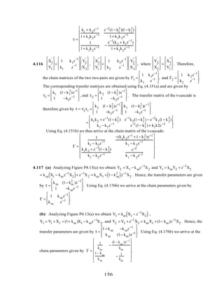
164. (b) A3(z) =
0.4 + 0.3z
–1
+ 0.2z
–2
+ z
–3
1+ 0.2z
–1
+ 0.3z
–2
+ 0.4z
–3 . Thus, k3 = 0.4 <1. A2(z) =
0.2619 + 0.0952z
–1
+ z
–2
1+ 0.0952z
–1
+ 0.2619z
–2 .
This implies, k2 = 0.2619 < 1. Next, A1(z) =
0.0755 + z
–1
1+ 0.0755z
–1 . Hence, k1 = 0.0755 <1. Since
ki < 1, for i = 3, 2, 1, Db(z) has all roots inside the unit circle.
4.124 z =
1 + s
1 − s
. Hence, s =
z − 1
z + 1
. Thus, the k-th root in the s-domain is given by
sk =
(zk −1)(zk
* +1)
zk +1
2 =
zk
2
−1+ zk − zk
*
zk + 1
2 where zk is the k-th root in the z-domain. Hence,
Re{sk} =
zk
2
−1
zk +1
2 . Since D(z) is a minimum phase polynomial, zk < 1. Therefore,
Re{sk} < 0. Hence B(s) is a strictly Hurwitz polynomial.
4.125 H(z) = 1− αz−1
. Hence, using Eq. (4.212) we get
Φyy(z) = H(z)H(z−1
)Φyy(z) = (1− αz−1
)(1 − α z)σx
2
. Therefore, from Eq. (4.214) we have
Pyy(ω) = H(ejω
)
2
Pxx(ω) = H(ejω
)
2
σx
2
= (1− α e−jω
)(1 − α ejω
)σx
2
= (1 + α2
− 2α cosω)σx
2
.
Now, H(z)H(z−1
) = (1− αz−1
)(1− α z) = −α z + (1+ α2
) − α z−1
. Hence,
φyy[n] = − αδ[n +1] + (1+ α2
)δ[n]− αδ[n −1]( )σx
2
.
As a result, average power = φyy[0]= (1+ α2
)σx
2
. Note that the average power increases with
increasing α .
4.126 H(z) =
1
1− 0.5z−1 . H(ejω
)
2
=
1
(1− 0.5e−j ω
)(1− 0.5ejω
)
=
1
1.25 − cosω
. Hence, rom Eq.
(4.214) we have Pyy(ω) = H(ejω
)
2
Pxx(ω) =
Pxx(ω)
(1− 0.5e−jω
)(1− 0.5ejω
)
=
σx
2
1.25 − cosω
. Now,
H(z)H(z−1
) =
1
1− 0.5z−1 ⋅
1
1− 0.5z
= −
z−1
(1 − 0.5z−1
)(0.5 − z−1
)
= −
2z−1
(1− 0.5z−1
)(1 − 2z−1
)
=
4 / 3
1− 0.5z−1 −
4 / 3
1 − 2z−1 . Therefore, ϕyy[n] =
4σx
2
3
(0.5)n
µ[n]+ (2)n
µ[−n −1]( ).
4.127 (a) Pyy(ω) = A(e
jω
)
2
Pxx(ω) =
A(e jω
)
2
1+ dcos(ω)
=
1
1+ dcos(ω)
. (16)
(b) No, The answer does not depend upon the choice of α . However Eq. (16) holds if the
filter is stable for which we require α < 1.
160

165. 4.128 (a) φxy[l] = E x[n + l ]y[n]{ } = E x[n + l]x[n]{ } * h[n] = φxx[n] * h[n]. Taking the discrete-
time Fourier transform of both sides we get Pxy(ω) = Pxx(ω)H(e
jω
). Since H(ejω
) in
general is not real, Pxy(ω) in general is not real.
(b) φxu[l] = E x[n + l ]u[n]{ } = E {x[n + l ]h[−n] * y[n]} = φxx[n] * h[n] * h[–n]. Taking the
discrete-time Fourier transform of both sides we get Pxu(ω) = Pxx(ω)H(e
jω
)
2
. Thus, Pxu(ω)
is a real function of ω .
M4.1 From Table 3.2, the DTFT of {n h[n]} is j
dH(e
jω
)
dω
. Hence, the group delay t(w) using Eq.
(4.203) can be computed at a set of N discrete frequency points wk = 2πk/N, k = 0, 1, . . . ,
N–1, as follows: {t(wk)} = Re(DFT{n h[n]}/DFT{h[n]}), where all DFTs are N-points in length
with N greater than or equal to length of {h[n]}.
M4.2 We modify Program 4_2 using the following statements:
b = [-4.8788 9.5631 -4.8788];
x1 = cos(0.2*n);x2=cos(0.5*n);
0 20 40 60 80
-1.5
-1
-0.5
0
0.5
1
1.5
2
Time index n
M4.3 We modify Program 4_2 using the following statements:
b = [-13.4866 45.228 -63.8089 45.228 -13.4866];
zi = [0 0 0 0];
x1 = cos(0.2*n);x2=cos(0.5*n);x3 = cos(0.8*n);
y=filter(b,1,x1+x2+x3,zi);
0 20 40 60 80
-1.5
-1
-0.5
0
0.5
1
1.5
2
Time index n
161

166. M4.4
M4.5 (a) num1 = [0 0.75 2 2 1 0.75];
num2 = [0 -0.75 2 -2 1 -0.75];
den = [3 0 3.5 0 1];
w = 0:pi/255:pi;
h1 = freqz(num1, den, w);
h2 = freqz(num2, den, w);
plot(w/pi, abs(h1).*abs(h1)+abs(h2).*abs(h2));
(b) Replace the first three lines in the above MATLAB program with the following:
num1 = [1 1.5 3.75 2.75 2.75 3.75 1.5 1];
num2 = [1 -1.5 3.75 -2.75 2.75 -3.75 1.5 -1];
den = [6 0 6.5 0 4.75 0 1];
M4.6 The magnitude response of H(z) is as shown below from which we observe that H(z) is a
lowpass filter.
By multiplying out the factors of H(z) we get
H(z) =
0.05634 –0.000935z
–1
+ 0.000935z
–2
+ 0.05634z
–3
1– 2.1291z
–1
+1.783386 z
–2
+ 0.543463z
–3 , The corresponding difference
equation representation is therefore given by
y[n] = 0.05634x[n]– 0.000935x[n –1]+ 0.000935x[n – 2]– 0.05634x[n –3]
–2.1291y[n –1]+ 1.783386y[n – 2]+ 0.543463y[n –3].
M4.7 The magnitude response of H(z) is as shown below from which we observe that H(z) is a
highpass filter.
162

167. By multiplying the factors of H(z) we get
H(z) =
1− 4z−1
+ 6z−2
− 4z−3
+ z−4
1− 3.0538 z−1 + 3.8227z−2 − 2.2837z−3 + 0.5472 z−4
The correspondong difference equation is given by
y[n]− 3.0538y[n −1]+ 3.8227y[n − 2]− 2.2837y[n − 3]+ 0.5472 y[n − 4]
= x[n]− 4x[n −1]+ 6x[n− 2]− 4x[n − 3]+ x[n − 4].
M4.8 From Eq. (4.66), we obtain M = –
1
2log2 (cos(0.12π)
= 4.7599. We choose M = 5. A cascade
of 5 first-order lowpass FIR filter has a transfer function given by G(z) =
1
32
(1+ z
–1
)
5
, whose
gain response is plotted below:
M4.9 For a cascade of M sections of the first-order highpass FIR filter of Eq. (4.67), the 3-dB
cutoff frequency wc is given by ωc = 2sin
–1
2
–1/ 2M
( ). Hence, M = –
1
2log2 (sin(ωc / 2)
.
Substituting the value of ωc we then obtain M = 4.76. Choose M = 5. A cascade of 5 first-
order highpass FIR filter has a transfer function given by G(z) =
1
32
(1– z
–1
)
5
, whose gain
response is plotted below:
163

168. M4.10 From Eq. (4.72b), we obtain α = 0.32492. Hence, from Eq. (4.70) we get
HLP(z) =
0.33754(1+ z
–1
)
1–0.32492z
–1 . Likewise, from Eq. (4.73) we get HHP(z) =
0.66246(1– z
–1
)
1– 0.32492z
–1 .
The magnitude responses of HLP(z) and HHP(z) are show below:
The magnitude response of HLP(z) + HHP(z) is shown below on the left-hand side, while the
gain response of HLP (e
jω
)
2
+ HHP (e
jω
)
2
is shown below on the right-hand side:
M4.11 From Eq. (4.76) we first obtain b = 0.309017. From Eq. (4.77) we arrive at two possible
values of a: 0.6128 and 1.63185 leading to two posible solutions:
HBP
'
(z) =
0.1935(1– z
–2
)
1– 0.4984 z
–1
+ 0.6128z
–2 , and HBP
"
(z) =
–0.3159(1– z
–2
)
1– 0.813287z
–1
+1.63185z
–2 . It can be
seen that HBP
"
(z) is unstable. From Eq. (4.79), the bandstop transfer function corresponding to
164

169. HBP
'
(z) is given by HBS
'
(z) =
0.8064(1–0.6180z
–1
+ z
–2
)
1– 0.498383z
–1
+ 0.6128z
–2 . A plot of the magnitude responses
of HBP
'
(z) and HBS
'
(z) are given below:
The magnitude response of HBP(z) + HBS(z) is shown below on the left-hand side, while the
gain response of HBP(e
jω
)
2
+ HBS(e
jω
)
2
is shown below on the right-hand side:
M4.12 From Eq. (4.76), we first obtain b = 0.309017. From Eq. (4.77) we arrive at two possible
values of a: 1.376381 and 0.72654253 leading to two posible solutions:
HBP
'
(z) =
0.1935996(1– z
–2
)
1+ 0.94798z
–1
+ 0.6128z
–2 , and HBP
"
(z) =
–0.3159258(1– z
–2
)
1+1.5469636z
–1
+ 1.63185168z
–2 .
It can be seen that HBP
"
(z) is unstable. A plot of the gain response of HBP
'
(z) is shown below:
M4.13 From Eq. (4.76), we first obtain b = 0.309016. From Eq. (4.77) we arrive at two possible
values of a: 0.72654253 and 1.376382 leading to two posible solutions:
165

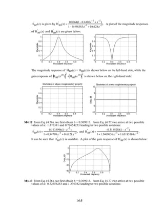
170. HBS
'
(z) =
0.86327126(1+ 0.618033z
–1
+ z
–2
)
1– 0.533531z
–1
+ 0.72654253z
–2 , and HBS
"
(z) =
1.188191(1+ 0.618033z
–1
+ z
–2
)
1– 0.7343424z
–1
+1.376382 z
–2 .
It can be seen that HBS
"
(z) is unstable. A plot of the gain response of HBS
"
(z) is shown below:
M4.14 (a) Using the following program we arrive at the two plots shown below:
b1 = [2 2]; b2 = [1 -1]; den = [3 1];
w = 0:pi/255:pi;
h1 = freqz(b1, den, w); h2 = freqz(b2, den, w);
sum = abs(h1).*abs(h1)+abs(h2).*abs(h2);
subplot(2,1,1);
plot(w/pi,abs(h1+h2));grid
axis([0 1 0 1.2]);
xlabel('Normalized frequency');ylabel('Magnitude');
title('Illustration of allpass complementary property');
subplot(2,1,2);
plot(w/pi,20*log10(sum));grid
axis([0 1 -10 10]);
xlabel('Normalized frequency');ylabel('Gain, dB');
title('Illustration of power complementary property');
(b) For this part, replace the first line in the above program with the following:
b1 = [–1 0 1]; b2 = [3 2 3]; den = [4 2 2];
166

171. M4.15 (a)
(b)
(c)
(d)
167

172. (e)
(f)
M4.16 (a) (b)
(c) (d)
168

173. (e)
M4.17 (a) The stability test parameters are
0.0833 -0.2098 -0.6106
stable = 1
(b) The stability test parameters are
–0.3333 1.0000 2.0000
stable = 0
(c) The stability test parameters are
0.0278 0.2317 0.6503 0.9147
stable = 1
(d) The stability test parameters are
0.0312 0.2346 0.6225 0.8726 0.9630
stable = 1
(e) The stability test parameters are
0.1667 0.0286 0.3766 0.3208 0.5277
stable = 1
M4.18 (a) The stability test parameters are
0.2000 0.2500 0.3333 0.5000
stable = 1
(b) The stability test parameters are
0.4000 0.2619 0.0755
stable = 1
M4.19 H(z) = –
k
4
+ 1+
k
2





 z–1
–
k
4
z–2
.
M4.20 H(z) = –
k2
4
+
k1
4
z–1
+ 1–
k1
2
+
k2
2





 z–2
+
k1
4
z–3
–
k2
4
z–4
.
169

174. 170

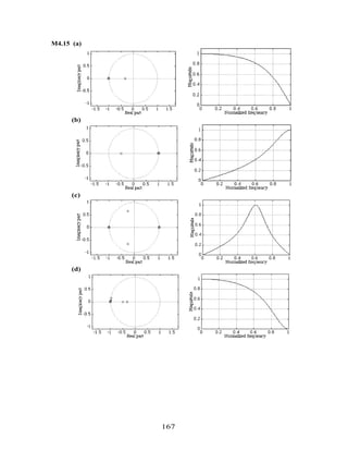
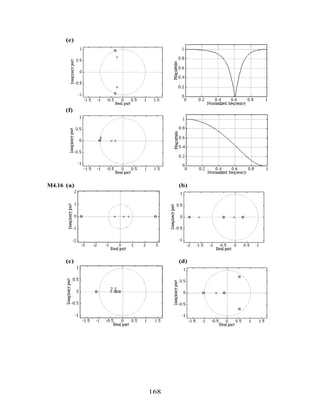
175. Chapter 5 (2e)
5.1 p(t) = δ(t − nT)
n=−∞
∞
∑ . Since p(t) is periodic function of time t with a period T, it can be
represented as a Fourier series: p(t) = cne
j(2πnt/ T)
n=−∞
∞
∑ , where cn = δ(t)e
−j(2πnt/ T)
dt
−T / 2
T/ 2
∫ =
1
T
.
Hence p(t) = δ(t − nT)
n=−∞
∞
∑ =
1
T
e
j(2πnt / T)
n=−∞
∞
∑ .
5.2 Since the signal xa(t) is being sampled at 1.5 kHz rate, there will be multiple copies of the
spectrum at frequencies given by Fi ± 1500 k, where Fi is the frequency of the i-th sinusoidal
component in xa(t). Hence,
F1 = 250 Hz, F1m = 250, 1250, 1750, . . . . , Hz
F2 = 450 Hz, F2m = 450, 1050, 1950 . . . . , Hz
F3 = 1000 Hz, F3m = 1000, 500, 2500 . . . . , Hz
F4 = 2750 Hz, F4m = 2750, 1250, 250, . . . .,Hz
F5 = 4050 Hz, F5m = 34050, 1050, 450, . . . .,Hz
So after filtering by a lowpass filter with a cutoff at 750 Hz, the frequencies of the sinusoidal
components present in ya(t) are 250, 450, 500 Hz.
5.3 One possible set of values are F1 = 450 Hz, F2 = 625 Hz, F3 = 950 Hz and F4 = 7550 Hz.
Another possible set of values are F1 = 450 Hz, F2 = 625 Hz , F3 = 950 Hz, F4 = 7375 Hz.
Hence the solution is not unique.
5.4 t = nT =
n
4000
. Therefore,
x[n]= 3cos
400π n
4000





 + 5sin
1200 πn
4000





 + 6cos
4400π n
4000





 + 2sin
5200 π n
4000






= 3cos
πn
10





 + 5sin
3πn
10





 + 6cos
11π n
10





 + 2sin
13 πn
10






= 3cos
πn
10





 + 5sin
3πn
10





 + 6cos
(20 − 9)π n
10





 + 2sin
(20 − 7)π n
10






= 3cos
πn
10





 + 5sin
3πn
10





 + 6cos
9π n
10





 − 2sin
7π n
10





 .
5.5 Both the channels are sampled at 48.2 kHz. Therefore there are a total of 2× 48200 = 96400
samples/sec. Each sample is quantized using 15 bits. Hence the total bit rate of the two
channels after sampling and digitization = 15× 96400 = 1.446 Mb/s.
5.6 hr(t) =
sin(Ωct)
(ΩTt / 2)
. Thus, hr(nT) =
sin(ΩcnT)
(ΩT nT / 2)
, Since T =
2π
ΩT
, hence hr(nT) =
sin
2πΩcn
ΩT








πn
.
If Ωc = ΩT / 2, then, hr(nT) =
sin(πn)
πn
= δ[n].
5.7 After sampling the spectrum of the signal is as indicated below:
171

176. T =
2π
2Ωm
=
π
Ωm
. As a result, ωc =
Ωmπ
3Ωm
=
π
3
. Hence after the low pass filtering the spectrum
of the signal will be as shown below:
5.8 (a) Ω2 = 200π, Ω1 =160 π. Thus, ∆Ω = Ω2 − Ω1 = 40π. Note ∆Ω is an integer multiple of
Ω2 . Hence, we choose the sampling angular frequency as
ΩT = 2∆Ω = 2(Ω2 − Ω1) = 80 π =
2 × 200 π
M
, which is satisfied for M = 5. The sampling
frequency is therefore FT = 40 Hz.
Xp ( jΩ)
Ω
40 π 80 π 120π 160π 200π0−40 π−80 π−160 π
−120 π
↑
M = 5
(b) Ω2 = 160π, Ω1 =120 π. Thus, ∆Ω = Ω2 − Ω1 = 40π. Note ∆Ω is an integer multiple of
Ω2 . Hence, we choose the sampling angular frequency as
ΩT = 2∆Ω = 2(Ω2 − Ω1) = 80 π =
2 × 160π
M
, which is satisfied for M = 4. The sampling
frequency is therefore FT = 40 Hz.
Ω
40π 80 π 120 π 160 π 200 π0
Xp ( jΩ)
−40 π−80 π−160 π
−120 π
↑
M = 4
172

177. (c) Ω2 = 150π, Ω1 =110 π. Thus, ∆Ω = Ω2 − Ω1 = 40π. Note ∆Ω is not an integer multiple
of Ω2 . Hence, we extend the bandwidth to the left by assuming the lowest frequency to be Ω0
andchoose the sampling angular frequency satisfying the equation
ΩT = 2∆Ω = 2(Ω2 − Ω0 ) =
2 ×150 π
M
, which is satisfied for Ω0 = 100π and M = 3. The
sampling frequency is therefore FT = 50 Hz.
Xp (jΩ)
Ω
0
M = 3
50 π− 50 π
5.9 αp = −20log10(1− δp ) and αs = −20 log10 δs . Therefore, δp = 1− 10
−αp/ 20
and δs = 10
−αs /20
.
(a) αp = 0.15, αs = 43., Hence, δp = 0.0171 and δs = 0.0071
(b) αp = 0.04, αs = 57. Hence, δp = 0.0046 and δs = 0.0014
(c) αp = 0.23, αs = 39. Hence, δp = 0.0261 and δs = 0.0112
5.10 H1(s) =
a
s + a
. Thus, H1(jΩ) =
a
jΩ + a
, and hence, i.e. H1(jΩ)
2
=
a
2
a
2
+ Ω
2 .
H1(jΩ)
2
is a monotonically decreasing function with H1(j0) = 1 and H1(j∞) = 0. Let the
3-dB cutoff frequency be given by Ωc . Then, H1(jΩc )
2
=
a
2
a
2
+ Ωc
2 =
1
2
, and hence, Ωc = a..
5.11 H2(s) =
s
s + a
. Thus, H2(jΩ) =
jΩ
jΩ+ a
, and hence, H2(jΩ)
2
=
Ω
2
a
2
+ Ω
2 .
H2(jΩ)
2
is a monotonically increasing function with H2 (j0) = 0 and H2 (j∞) = 1. The 3-
dB cutoff frequency is given by
Ωc
2
a
2
+ Ωc
2
=
1
2
, and hence, Ωc = a..
5.12 H1(s) =
a
s + a
=
1
2
1−
s − a
s + a





 , and H2(s) =
s
s + a
=
1
2
1+
s − a
s + a





. Thus, A1(s) = 1 and A2(s) =
s − a
s + a
. Since A1(jΩ) = 1 and A2(jΩ) = 1 ∀Ω hence A1(s) and A2(s) are both allpass
functions.
5.13 H1(s) =
bs
s
2
+ bs + Ωo
2 . Thus, H1(jΩ) =
jbΩ
jbΩ+ Ω0
2
− Ω
2 , hence H1(jΩ)
2
=
b2
Ω2
b2
Ω2
+ (Ω0
2
− Ω2
)2 .
Now at Ω = 0, H1(j0) = 0 and at Ω = ∞, H1(j∞) = 0 and at Ω = Ωo, H1(jΩo ) = 1. Hence
173

178. H1(s) has a bandpass response. The 3-dB frequencies are given by
b
2
Ωc
2
b
2
Ωc
2
+ (Ω0
2
− Ω
2
)
2 =
1
2
.
Thus, (Ωo
2
− Ωc
2
)
2
= b
2
Ωc
2
or Ωc
4
− (b
2
+ 2Ωo
2
)Ωc
2
+ Ωo
4
= 0. Hence if Ω1 and Ω2 are the roots
of this equation, then so are –Ω1, – Ω2,and the product of the roots is Ωo
4
. This implies
Ω1Ω2 = Ωo
2
. Also Ω1
2
+ Ω2
2
= b
2
+ 2Ωo
2
. Hence (Ω2 − Ω1)
2
= b
2
which gives the desired result
Ω2 − Ω1 = b.
5.14 H2(s) =
s
2
+ Ωo
2
s
2
+ bs+ Ωo
2 . Thus, H2(jΩ) =
Ωo
2
− Ω
2
Ωo
2
− Ω
2
+ jbΩ
, hence, H2(jΩ)
2
=
(Ω
2
− Ωo
2
)
2
(Ω
2
− Ωo
2
)
2
+ b
2
Ω
2 .
Now, H2(j0) =1, H2(j∞) = 1 and H2(jΩo) =1. Hence, H2(s) has a bandstop response. As in
the earlier problem one can show that Ω1Ω2 = Ωo
2
and also Ω2 − Ω1 = b.
5.15 H1(s) =
1
2
1−
s
2
− bs + Ωo
2
s
2
+ bs + Ωo
2







 =
1
2
A1(s)− A2(s){ } and H2(s) =
1
2
1+
s
2
− bs+ Ωo
2
s
2
+ bs+ Ωo
2







 =
1
2
A1(s)+ A2(s){ }. Thus, A1(s) = 1 and A2(s) =
s
2
− bs + Ωo
2
s
2
+ bs + Ωo
2 . Now
A2(jΩ)
2
=
(Ωo
2
− Ω
2
)
2
+ b
2
Ω
2
(Ωo
2
− Ω
2
)
2
+ b
2
Ω
2 = 1, and is hence A2(s) is an allpass function. A1(s) is seen
to be an allpass function.
5.16 Ha(jΩ)
2
=
1
1+ (Ω /Ωc)
2N .
dk(1/Ha(jΩ)
2
)
dΩk = 2N(2N –1)L(2N – k + 1)
Ω2N– k
Ωc
2N . Therefore
d
k
(1/Ha(jΩ)
2
)
dΩ
k
Ω=0
= 0 for k = 1, 2, . . . , 2N–1. or, equivalently,
d
k
(Ha(jΩ)
2
)
dΩ
k
Ω=0
= 0 for
k = 1, 2, . . . , 2N–1.
5.17 10 log10
1
1+ ε
2





 = –0.5,, which yields ε = 0.3493. 10 log10
1
A2





 = –30, which yields
A2
= 1000. Now,
1
k
=
Ωs
Ωp
=
8
2.1
= 3.8095238 and
1
k1
=
A2
–1
ε
=
999
0.3493
= 90.486576. Then,
from Eq. (5.33) we get N =
log10 (1/ k1)
log10(1/ k)
=
90.4866
3.8095
= 3.3684. Hence choose N = 4 as the order.
5.18 The poles are given by pl = Ωce
j
π(N+2l −1)
2N ,l = 1, 2,K,N. Here, N = 5 and Ωc = 1. Hence
p1 = ej 6 π/10
= −0.3090 + j0.9511, p2 = ej 8 π/10
= −0.8090 + j 0.5878, p3 = ej10 π/10
= −1,
p4 = ej12 π/10
= − 0.8090 - j 0.5878 = p2
*
, and p5 = ej 6 π/10
= −0.3090 - j0.9511= p1
*
.
174

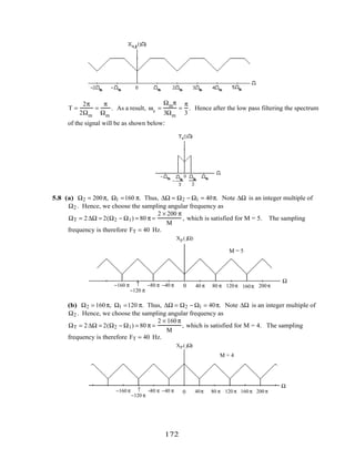
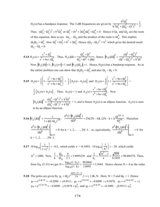
179. 5.19 From Eq. (5.39) TN (x) = 2xTN−1(x) − TN −2 (x) where TN (x) is defined in Eq. (5.38).
Case 1: x ≤ 1. Making use of Eq. (5.38) in Eq. (5.39) we get
TN (x) = 2xcos (N −1)⋅ cos−1
(x)( )− cos (N − 2) ⋅cos−1
(x)( )
= 2xcos(Ncos−1
x − cos−1
x) − cos(N cos−1
x − 2cos−1
x)
= 2x cos(N cos−1
x)cos(cos−1
x) + sin(Ncos−1
x)sin(cos−1
x)[ ]
− cos(N cos−1
x)cos(2cos−1
x) + sin(Ncos−1
x)sin(2cos−1
x)[ ]
= 2xcos(Ncos−1
x)⋅cos( cos−1
x) − cos(Ncos−1
x)⋅cos(2cos−1
x)
= 2x2
cos(Ncos−1
x) − cos(Ncos−1
x)⋅ 2cos2
(cos−1
x) −1[ ]
= cos(Ncos−1
x) 2 x2
− 2x2
+ 1[ ]= cos(N cos−1
x).
Case 2: x > 1. Making use of Eq. (5.38) in Eq. (5.39) we get
TN (x) = 2xcosh (N − 1)⋅ cosh−1
(x)( )− cohs (N − 2)⋅ cosh−1
(x)( ). Using the trigonometric
identities cosh (A − B) = cosh(A)cosh(B) − sinh (A)sinh (B), sinh (2A) = 2sinh (A)cosh(A), and
cosh (2A) = 2cosh2
(A) − 1, and following a similar algebra as in Case 1, we can show
TN (x) = 2xcosh (N − 1)⋅ cosh−1
(x)( )− cohs (N − 2)⋅ cosh−1
(x)( )= cosh(N cosh−1
x).
5.20 10 log10
1
1+ ε
2





 = –0.5,, which yields ε = 0.3493. 10 log10
1
A
2





 = –60, which yields A2 =
1000. Now,
1
k
=
Ωs
Ωp
=
8
2.1
= 3.8095238 and
1
k1
=
A2
–1
ε
=
999
0.3493
= 90.486576.. Then,
from Eq. (5.41) we get N =
cosh−1
(1 / k1)
cosh−1
(1/ k)
=
cosh−1
(90.486576)
cosh−1
(3.8095238)
=
5.1983
2.013
= 2.5824. We thus
choose N = 3 as the order.
5.21 From Problem 5.18 solution, we observe
1
k
= 3.8095238 or k = 0.2625, and
1
k1
= 90.4865769
or k1 = 0.011051362. Substituting the value of k in Eq. (5.52a) we get k' = 0.964932. Then,
from Eq. (5.52b) we arrive at ρo = 0.017534. Substituting the value of in Eq. (5.52c) we get
ρ = 0.017534. Finally from Eq. (5.51) we arrive at N = 2.9139. We choose N = 3.
5.22 From Eq. (5.53) BN(s) = (2N –1)BN–1(s) +s
2
BN–2 (s), where B1(s) = s + 1 and B2(s) = s2 +3s +
3. Thus, B3(s) = 5B2(s)+ s
2
B1(s) = 5(s
2
+ 3s + 3)+ s
2
(s +1) = s
3
+ 6s
2
+ 15s + 15, and
B4(s) = 7B3(s)+ s
2
B2(s) = 7(s
3
+ 6s
2
+15s +15) + s
2
(s
2
+ 3s + 3) = s
4
+10s
3
+ 45s
2
+105s + 105.
Thus, B5(s) = 9B4(s) + s2
B3 (s) = 9(s4
+ 10s3
+ 45s2
+105s + 105) + s2
(s3
+ 6s2
+15s + 15)
= s5
+ 15s4
+ 105s3
+ 420s2
+ 945s + 945, and
175

180. B6(s) = 11B5(s) + s2
B4 (s) = 11(s5
+ 15s4
+ 105s3
+ 420s2
+ 945s + 945,)
+ s2
(s4
+ 10s3
+ 45s2
+ 105s +105) = s6
+ 21s5
+ 210s4
+ 1260s3
+ 4725s2
+ 10395s + 10395.
5.23 We use the lowpass-to-highpass transformation given in Eq. (5.59) where now
Ωp = 2π(0.2) = 0.4π and ˆΩ p = 2π(2) = 4π. Therefore, from Eq. (5.59) we get the desired
transformation as s →
Ωp
ˆΩ p
s
=
1.6π2
s
=
15.791367
s
. Therefore,
HHP (s) = HLP (s)s→
15.791367
s
=
4.52
15.791367
s






2
+ 3
15.791367
s





 + 4.52
=
4.52 s2
4.52s2
+ 47.3741s + 2.49367
.
5.24 We use the lowpass-to-bandpass transformation given in Eq. (5.61) where now
Ωp = 2π(0.16) = 0.32π, ˆΩ o = 2π(3) = 6π, and ˆΩ p2 − ˆΩ p1 = 2π(0.5) = π. Substituting these
values in Eq. (5.59) we get the desired transformation s → 0.32π
s2
+ 36 π2
π s





 =
s2
+ 36 π2
3.125s
.
Therefore HBP(s) = HLP (s) s→
s2
+36π2
3.125 s
=
0.056
s2
+ 36 π2
3.125s






2
+17.95








s2
+ 36π2
3.125s






2
+ 1.06
s2
+ 36π2
3.125s





 + 1.13
=
0.056(s4
+ 49.61s2
+ 70695.62)
s4
+ 3.3125s3
+ 721.64667s2
+ 1176.95s + 126242.182
.
5.25 ˆΩ p = 2π(5) ×106
, ˆΩ s = 2 π(0.5) × 106
, ˆα p = 0.3 dB and ˆαs = 45 dB. From Figure 5.14 we
observe 10 log10
1
1+ ε2





 = −0.3, hence, ε2
= 100.03
− 1= 0.0715193, or ε = 0.26743. From
Figure 5.14 we also note that 10 log10
1
A2





 = −45, and hence A2
= 104.5
= 31622.7766. Using
these values in Eq. (5.30) we get k1 =
ε
A2
− 1
= 0,001503898.
To develop the bandedges of the lowpass prototype, we set Ωp = 1 and obtain using Eq. (5.59)
Ωs =
ˆΩ p
ˆΩ s
=
5
0.5
= 10. Next, using Eq. (5.29) we obtain k =
Ωp
Ωs
=
1
10
= 0.1. Substituting the
values of k and k1 in Eq. (5.33) we get N =
log10 (1/ k1)
log10(1/ k)
= 2.82278. We choose N = 3 as the
order of the lowpass filter which is also the order of the highpass filter.
To verify using MATLAB er use the statement
[N,Wn] = buttord(1,10,0.3,45,'s')
which yields N = 3 and Wn = 1.77828878.
176

181. 5.26 ˆFp1 = 20 ×103
, ˆFp2 = 45 × 103
, ˆFs1 = 10 × 103
, ˆFs2 = 60 ×103
, αp = 0.5 dB and αs = 40 dB.
We observe ˆFp1
ˆFp2 = 20 × 45 × 106
= 9 ×108
, and ˆFs1
ˆFs2 = 10 × 60 × 106
= 6 × 108
. Since
ˆFs1
ˆFs2 ≠ ˆFp1
ˆFp2 , we adjust the the stopband edge on the left to ˆFs1 = 15 ×103
in which case
ˆFs1
ˆFs2 = ˆFp1
ˆFp2 = Fo
2
= 9 ×108
. The angular center frequency of the desired bandpass filter is
therefore Ωo = 2π Fo = 2π × 30 × 103
. The passband bandwidth is
Bw = ˆΩ p2 − ˆΩ p1 = 2π × 25 ×103
.
To determine the banedges of the prototype lowpass filter we set Ωp = 1 and then using Eq.
(5.62) we obtain Ωs = Ωp
ˆΩ o
2
− ˆΩ s1
2
ˆΩ s1Bw
=
302
− 152
15 × 25
= 1.8. Thus, k =
Ωp
Ωs
=
1
1.8
= 0.5555555556 .
Now, 10 log10
1
1+ ε2





 = −0.5, and hence, ε2
= 100.05
− 1= 0.1220184543, or ε = 0.34931140019.
In addition 10 log10
1
A2





 = −40 or A2
= 104
= 10000. Using these values in Eq. (5.30) we get
k1 =
ε
A2
− 1
= 0.00349328867069. From Eq. (5.52a) we get
k' = 1 − k2
= 0.831479419283,and then from Eq. (5.52b) we get
ρo =
1 − k'
2(1 + k' )
= 0.02305223718137. Substituting the value of ρo in Eq. (5.52c) we then get
ρ = 0.02305225. Finally, substituting the values of ρ and k1 in Eq. (5.51) we arrive at
N =
2log10 (4 / k1)
log10(1/ ρ)
= 3.7795. We choose N = 4 as the order for the prototype lowpass filter.
The order of the desired bandpass filter is therefore 8.
Using the statement [N,Wn]=ellipord(1,1.8,0.5,40,'s') we get N = 4 and
Wn = 1.
5.27 ˆFp1 =10 ×106
, ˆFp2 = 70 × 106
, ˆFs1 = 20 × 106
, and ˆFs2 = 45 × 106
, We observe
ˆFp1
ˆFp2 = 700 ×1012
, and ˆFs1
ˆFs2 = 900 ×1012
. Since ˆFp1
ˆFp2 ≠ ˆFs1
ˆFs2 . we adjust the right
stopband edge to ˆFs2 = 35 × 106
, in which case ˆFp1
ˆFp2 = ˆFs1
ˆFs2 = ˆFo
2
= 700 × 1012
. The
stopband bandwidth is Bw = ˆΩ s2 − ˆΩ s1 = 2π × 15 ×106
.
177

182. Now, 10 log10
1
1+ ε2





 = −0.5, and hence, ε2
= 100.05
− 1= 0.1220184543, or ε = 0.34931140019.
In addition 10 log10
1
A2





 = −30 or A2
= 103
= 1000. Using these values in Eq. (5.30) we get
k1 =
ε
A2
− 1
= 0.01105172361656.
To determine the banedges of the prototype lowpass filter we set Ωs = 1 and then using Eq.
(5.65) we obtain Ωp = Ωs
ˆΩ s1Bw
ˆΩ o
2
− ˆΩ s1
2 = 0.3157894. Therefore, k =
Ωp
Ωs
= 0.3157894.
Substituting the values of k and k1 in Eq. (5.41) we get N =
cosh−1
(1 / k1)
cosh−1
(1/ k)
= 2.856. We choose
N = 3 as the order for the prototype lowpass filter.
The order of the desired bandstop filter is therefore 6.
Using the statement [N,Wn] = cheb1ord(0.3157894,1,0.5,30,'s') we get
N = 3 and Wn = 0.3157894.
5.28 From Eq. (5.59), the difference in dB in the attenuation levels at Ωp and Ωo is given by
20N log10
Ωo
Ωp







 . Hence for Ωo = 2Ωp, attenuation difference in dB is equal to 20N log10 2 =
6.0206 N. Likewise, for Ωo = 3Ωp, attenuation difference in dB is equal to 20N log10 3 =
9.5424 N. Finally, for Ωo = 4Ωp,attenuation difference in dB is equal to 20N log10 4 =
12.0412 N.
5.29 The equivalent representation of the D/A converter of Figure 5.39 reduces to the circuit shown
below if the l − th is ON and the remaining bits are OFF, i.e. al = 1, and ak = 0, k ≠ l.
2
N −1
2
l
2
l−1
2
l−2
2
0
al
VR
+
–
GL
Yin
V0,l
In the above circuit, Yin is the total conductance seen by the load conductance GL which is
given by Yin = 2i
i =0
N−1
∑ = 2N
−1. The above circuit can be redrawn as indicated below:
alVR
+
–
2
l−1 GLYin − 2
l−1
V0,l
178

183. Using the voltage divider relation we then get V0,l =
2l −1
Yi + GL
al VR. Using the superposition
theorem, the general expression for the output voltage V0 is thus given by
V0 =
2l −1
Yi + GL
al VR = 2l −1
al
RL
1+ (2N −1)RL








VR
l =1
N
∑
l =1
N
∑ .
5.30 The equivalent representation of the D/A converter of Figure 5.40 reduces to the circuit shown
below if the N-th bit is ON and the remaining bits are OFF, i.e. aN = 1, and ak = 0, k ≠ N.
aN
VR
+
–
V0,N
G
2
G
2
GL
which simplifies to the one shown below
aNVR
+
–
V0,N
G
2
G
2
+ GL
Using the voltage-divider relation we then get V0,N =
G
2
G
2
+ GL
+
G
2
aNVR =
R L
2(R + RL )
aN VR.
The equivalent representation of the D/A converter of Figure 5.40 reduces to the circuit shown
below if the (N–1)-th bit is ON and the remaining bits are OFF, i.e. aN–1 = 1, and ak = 0, k ≠
N.
V0 ,N−1
aN−1
VR
+
–
G
2
G
2
G
2
G L
G
The above circuit simplifies to the one shown below:
V0,N−1
aN−1VR
+
–
G
2
+ G L
G
G
2
G
2
Its Thevenin equivalent circuit is indicated below:
G
2
+
–
G
2
+ GL
V0,N−1
aN−1
2
VR
from which we readily obtain
179

184. V0,N−1 =
G
2
G + GL
aN −1
2
VR =
RL
2(RL + R)
aN−1
2
VR.
Following the same procedure we can show that if the l -th bit is ON and the remaining bits are
OFF, i.e. al = 1, and ak = 0, k ≠ l , then
V0,l =
RL
2(RL + R)
al
2N −l VR.
Hence, in general we have
V0 =
RL
2(RL + R)
al
2N−l VR
l =1
N
∑ .
5.31 From the input-output relation of the first-order hold we get the expression for the impulse
response as hf(t) = δ(nT) +
δ(nT) − δ(nT − T)
T
(t − nT), nT ≤ t < (n + 1)T. In the range 0 ≤ t < T ,
the impulse response is given by hf(t) = δ(0) +
δ(0) − δ(−T)
T
t =1 +
t
T
. Likewise, in the range
T ≤ t < 2T , the impulse response is given by hf(t) = δ(T) +
δ(T) − δ(T − T)
T
(t − T) = 1−
t
T
.
Outside these two ranges, hf(t) = 0. Hence we have
hf(t) =
1 +
t
T
, 0 ≤ t < T,
1−
t
T
T ≤ t < 2T,
0, otherwise.








t
hf (t)
1
2
–1
0 T 2T
Using the unit step function µ(t) we can write
hf(t) = 1+
t
T





 µ(t) − µ(t − T)[ ] + 1−
t
T





 µ(t − T) − µ(t − 2T)[ ]
= µ(t) +
t
T
µ(t) −
2(t − T)
T
µ(t − T) + 2µ(t − T) − µ(t − 2T) +
t − 2T
T





 µ(t − 2T) + 2µ(t − 2T).
Taking the Laplace transform of the above equation we arrive at the transfer function
Hf (s) =
1
s
+
1
Ts2 −
2
T
⋅
e−sT
s2 + 2
e−sT
s
−
e− 2sT
s
+
1
T
⋅
e− 2sT
s2 + 2
e−2 sT
s
=
1 + s T
T






1− e−sT
s






2
.
Hence, the frequency response is given by
Hf (jΩ) =
1+ jΩT
T






1− e− jΩT
jΩ






2
= T 1+ Ω2
T2 2sin(ΩT / 2)
ΩT






2
ej ΩT
etan−1
ΩT
.
180

185. A plot of the magnitude responses of the ideal filter, zero-order hold and the first-order hold is
shown below:
0 1 2 3
0
0.5
1
1.5
Ideal
First-order hold
Zero-order hold
Ω
5.32 From the input-output relation of the linear interpolator we get the expression for the impulse
response as hf(t) = δ(nT − T)+
δ(nT) − δ(nT − T)
T
(t − NT), nT ≤ t < (n + 1)T. In the range
0 ≤ t < T , the impulse response is given by hf(t) = δ(−T)+
δ(0)− δ(−T)
T
t, and in the range
T ≤ t < 2T , the impulse response is given by hf(t) = δ(0)+
δ(T)− δ(0)
T
(t − T), Outside these two
ranges, hf(t) = 0. Hence we have
hf(t) =
t
T
, 0 ≤ t < T,
2−
t
T
T ≤ t < 2T,
0, otherwise.








t
hf (t)
1
2
0 T 2T
Using the unit step function µ(t) we can write
hf(t) =
t
T
µ(t) − µ(t − T)[ ]+ 2 −
t
T





 µ(t − T) − µ(t − 2T)[ ]
=
t
T
µ(t) −
2(t − T)
T
µ(t − T) +
(t − 2T)
T
µ(t − 2T).
Taking the Laplace transform of the above equation we arrive at the transfer function
Hf(s) =
1
s2T
−
2e−sT
s2T
+
e−2sT
s2T
= T
1− e−sT
sT






2
. Hence, the frequency response is given by
Hf(jΩ) = T
1− e−jΩT
jΩT






2
= T
sin(ΩT/ 2)
ΩT / 2






2
e−jΩT
.
A plot of the magnitude responses of the ideal filter, zero-order hold and the first-order hold is
shown below:
181

186. 0 1 2 3
0
0.2
0.4
0.6
0.8
1
Ω
Ideal
Linear Interpolator
Zero-order hold
M5.1 Using the MATLAB statement
[N,Wn] = buttord(2*pi*2100, 2*pi*8000, 0.5, 30, 's')
we arrive at N = 4 and the 3-dB passband edge frequency Wn = 21199.429284 rad/sec.
M5.2 Using the MATLAB statement
[N,Wn] = cheb1ord(2*pi*2100, 2*pi*8000, 0.5, 30, 's')
we arrive at N = 3 and the passband edge frequency Wn = 13194.689145 rad/sec.
M5.3 Using the MATLAB statement
[N,Wn] = ellipord(2*pi*2100, 2*pi*8000, 0.5, 30, 's')
we arrive at N = 3 and the passband edge frequency Wn = 1.3194689145 rad/sec.
M5.4 We use N = 4 and Wn = 21199.429284 computed in Exercise M5.1 in Program M5_2
and use omega = 0:2*pi:2*pi*9000; to evaluate the frequency points. The gain plot
developed by running Program 5_2 is as shown below:
0 2000 4000 6000 8000 10000
-40
-30
-20
-10
0
10
Frequency, Hz
Analog Lowpass Filter
0 500 1000 1500 2000 2500
-1
-0.5
0
0.5
Frequency, Hz
Pasband Details
M5.5 We use N = 3 computed in Exercise M5.2 and and Fp = 2*pi*2100 and Rp = 0.5
in Program M5_3 and use omega = 0:2*pi:2*pi*8000; to evaluate the frequency
points. The gain plot developed by running Program 5_3 is as shown below:
182

187. 0 2000 4000 6000 8000
-50
-40
-30
-20
-10
0
Frequency, Hz
Analog Lowpass Filter
0 500 1000 1500 2000 2500
-1
-0.5
0
0.5
Frequency, Hz
Passband Details
M5.6 We replace the statement
Rp = input('Passband edge frequency in Hz = '); with
Rs = input('Stopband edge frequency in Hz = '); and replace
[num,den] = cheby1(N,Rp,Fp,'s'); with
[num,den] = cheby2(N,Rs,Fs,'s'); to modify Program 5_3 and use N = 3
computed in Exercise M5.2 and Rs = 30 in the modified Program M5_3 and use w =
0:2*pi:2*pi*8000; to evaluate the frequency points.
The gain plot developed by running the modified Program 5_3 is as shown below:
0 2000 4000 6000 8000
-60
-50
-40
-30
-20
-10
0
Frequency, Hz
Analog Lowpass Filter
0 500 1000 1500 2000 2500
-1
-0.5
0
0.5
Frequency, Hz
Passband Details
M5.7 We use N = 3 and Wn = 1.3194689145 computed in Exercise M5.3 in Program
M5_3 and use w = 0:2*pi:2*pi*9000; to evaluate the frequency points. The gain plot
developed by running Program 5_3 is as shown below:
0 2000 4000 6000 8000
-60
-50
-40
-30
-20
-10
0
Frequency, Hz
Analog Lowpass Filter
0 500 1000 1500 2000 2500
-1
-0.5
0
0.5
Frequency, Hz
Passband Details
M5.8 The MATLAB program used is as given below:
[N,Wn] = buttord(1,10,0.3,45,'s')
183

188. [B,A] = butter(N,Wn,'s')
[num,den] = lp2hp(B,A,2*pi*5e6)
figure(1)
omega = [0: 0.1: 20];
h = freqs(B,A,omega);
gain = 20*log10(abs(h));
plot (omega,gain);grid;axis([0 20 -80 5]);
xlabel('Omega'); ylabel('Gain, dB')
title('Analog Lowpass Filter')
figure(2)
omega = [0: 10000: 10e6*pi];
h = freqs(num,den,omega);
gain = 20*log10(abs(h));
plot (omega/(2*pi),gain);grid;axis([0 5e6 -80 5]);
xlabel('Frequency in Hz'); ylabel('Gain, dB')
title('Analog Highpass Filter')
HLP (s) =
5.6235
s3
+ 3.5566s2
+ 6.3246s + 5.6235
0 5 10 15 20
-80
-60
-40
-20
0
Ω
Analog Lowpass Filter
0 0.2 0.4 0.6 0.8 1
-1
-0.5
0
0.5
Ω
Passband Details
HHP (s) =
s3
+ 4.4345 × 10−9
s2
+ 9.0568 × 10−2
s + 4.2847 ×10−11
s3
+ 3.5333 ×107
s2
+ 6.242 × 1014
s + 5.5137 × 1021
0 1 2 3 4 5
x 10
6
-80
-60
-40
-20
0
Frequency in Hz
Analog Highpass Filter
3 4 5 6
x 10
6
-1
-0.5
0
0.5
Frequency in Hz
Passband Details
M5.9 The MATLAB program used is as given below:
[N,Wn] = ellipord(1,1.8,0.5,40,'s')
184

189. [B,A] = ellip(N,0.5,40,Wn,'s')
[num,den] = lp2bp(B,A,2*pi*30e3,2*pi*25e3)
figure(1)
omega = [0: 0.01: 4];
h = freqs(B,A,omega);
gain = 20*log10(abs(h));
plot (omega,gain);grid;axis([0 4 -80 5]);
xlabel('Omega'); ylabel('Gain, dB')
title('Analog Lowpass Filter')
figure(2)
omega = [0: 200: 200e3*pi];
h = freqs(num,den,omega);
gain = 20*log10(abs(h));
plot (omega/(2*pi),gain);grid;axis([0 100e3 -80 5]);
xlabel('Frequency in Hz'); ylabel('Gain, dB')
title('Analog Bandpass Filter')
HLP (s) =
0.01s4
+ 0.17921s2
+ 0.44866
s4
+ 1.1789s3
+ 1.7558s2
+1.0845s + 0.47524
0 1 2 3 4
-80
-60
-40
-20
0
Ω
Analog Lowpass Filter
0 0.2 0.4 0.6 0.8 1
-1
-0.5
0
0.5
Ω
Passband details
HBP(s) =
1.0002 ×10−2
s8
− 2.3081 × 10−12
s7
+ 5.8434 × 109
s6
− 6.4605 × 10−1
s5
+ 6.6313 ×1020
s4
− 3.9221 ×1010
s3
+ 7.3769 ×1030
s2
− 3.1971 × 1020
s + 1.5941× 1040
s8
+ 1.8519 × 105
s7
+1.8544 ×1011
s6
+ 2.3943 × 1016
s5
+ 1.0942 × 1022
s4
+8.507 × 1026
s3
+ 2.3411 × 1032
s2
+ 8.3065 × 1036
s + 1.5937 × 1042
0 2 4 6 8 10
x 104
-80
-60
-40
-20
0
Frequency in Hz
Analog Bandpass Filter
2 2.5 3 3.5 4 4.5
x 104
-1
-0.5
0
0.5
Frequency in Hz
Passband details
M5.10 The MATLAB program used is as given below:
[N,Wn] = cheb1ord(0.3157894,1,0.5,30,'s')
185

190. [B,A] = cheby1(N,0.5, Wn,'s')
[num,den] = lp2bs(B,A,2*pi*sqrt(700)*10^6,2*pi*15e6)
figure(1)
omega = [0: 0.01: 10];
h = freqs(B,A,omega);
gain = 20*log10(abs(h));
plot (omega,gain);grid;axis([0 4 -70 5]);
xlabel('Omega'); ylabel('Gain, dB')
title('Analog Lowpass Filter')
figure(2)
omega = [0: 100000: 160e6*pi];
h = freqs(num,den,omega);
gain = 20*log10(abs(h));
plot (omega/(2*pi),gain);grid;axis([0 80e6 -70 5]);
xlabel('Frequency in Hz'); ylabel('Gain, dB')
title('Analog Bandstop Filter')
HLP (s) =
0.022538
s3
+ 0.39566s2
− 0.15306s + 0.022538
0 1 2 3 4
-60
-40
-20
0
Ω
Analog Lowpass Filter
0 0.1 0.2 0.3 0.4 0.5
-1
-0.5
0
0.5
Ω
Passband Details
HBS(s) =
s6
− 2.6591× 10−8
s5
+ 8.2905 × 1016
s4
− 1.4698 × 109
s3
+ 2.2911 ×1033
s2
− 2.031× 1025
s + 2.1104 × 1049
s6
+ 6.4007 ×108
s5
+ 2.3884 ×1017
s4
+ 7.2521× 1025
s3
+ 6.6003 × 1033
s2
+ 4.8881× 1041
s + 2.1104 × 1049
0 2 4 6 8
x 10
7
-60
-40
-20
0
Frequency in Hz
Analog Bandstop Filter
0 2 4 6 8
x 107
-1
-0.5
0
0.5
Frequency in Hz
Passband Details
186

191. M5.11 The MATLAB program to generate the plots of Figure 5.48 is given below:
% Droop Compensation
w = 0:pi/100:pi;
h1 = freqz([-1/16 9/8 -1/16], 1, w);
h2 = freqz(9, [8 1], w);
w1 = 0;
for n = 1:101
h3(n) = sin(w1/2)/(w1/2);
w1 = w1 + pi/100;
end
m1 = 20*log10(abs(h1));
m2 = 20*log10(abs(h2));
m3 = 20*log10(abs(h3));
plot(w/pi, m3, 'r-',w/pi, m1+m3, 'b--',w/pi, m2+m3,'r-
');grid
xlabel('Normalized frequency');ylabel('Gain, dB');
text(0.43,-0.58,'DAC','sc');text(0.85,-0.58,'IIR','sc');
text(0.85,-1.67,'FIR','sc');
187

192. Chapter 6 (2e)
6.1 From Figure P6.1, we get w[n] = A(x[n]+ C Du[n]), and y[n] = C(A Bx[n]+ u[n]). These
two equations can be rewritten as w[n] = Ax[n]+ A C Du[n], and y[n] = CA Bx[n]+ Cu[n].
The corresponding realization shown below has no delay-free loop:
6.2 (a)
X(z)
Y(z)
X2(z) Y2 (z)Y3(z)X3(z)
k1
W(z)
k2
α1
α 2
Analyzing the above figure we get (1): W(z) = X(z) − α1Y3(z), (2): Y2 (z) = W(z) + k1Y2(z),
(3): Y3(z) = k2Y2(z) + X2(z), and (4): Y(z) = α2W(z) + X3(z).
From Eq. (2) we get (5): W(z) = (1− k1)Y2 (z). Substituting Eqs. (3) and (5) in Eq. (1) we get
(1− k2 )Y2 (z) = X(z) − α1 k2Y2 (z) + X2 (z)( ) or (6): Y2 (z) =
1
1− k1 + α1k2
X(z) − α1X2 (z)( ).
Substituting Eq. (5) in Eq. (4) we get (7): Y(z) = α2(1− k1)Y2(z) + X3(z).
A realization based on Eqs. (6), (7) and (3) shown below has no delay-free loops.
X(z)
Y(z)
X2(z)
Y2(z)
Y3(z)
X3(z) k2
α1–
z−1
z−1
1
1 − k1 + α1k2
α2 (1 − k1)
(b)
X(z) Y(z)
X 2(z)Y2 (z) Y3 (z) X3(z)
δ
γ
β
188

193. Analyzing the above figure we get (1): Y2 (z) = X(z) + δY(z), (2): Y3(z) = βY2 (z) + X2 (z),
and (3): Y(z) = X3(z) + γ Y2 (z). From Eqs. (1) and (3) we get
Y2 (z) = X1(z) + δ X(z) + γ Y2 (z)( ), which yields (4): Y2 (z) =
1
1− δ γ
δX(z) + X3(z)( ). Next,
substituting Eq. (4) in Eq. (3) we get
(5): Y(z) = X3(z) + γ Y2 (z) = X3(z) +
γ
1− δγ
X(z) + δX3(z)( ) =
1
1 − δγ
γ X(z) +X3(z)( ).
A realization based on Eqs. (2), (4) and (5) shown below has no delay-free loops.
X(z)
Y(z) X2(z)
Y2 (z)
Y3(z)X3(z)
δ
γ β z−1
z−1
6.3 H(z) =
G1(z)
1− G1(z)G2(z)
=
1
1− 2z−1
1 −
K
1− 2z−1
=
1
(1− K) − 2z−1 . The pole is at z =
2
1 − K
. Therefore, the
system is stable if
2
1− K
< 1, i.e. if −1> K > 3.
6.4
From the above figure, we get W1 = K X + z
−1
W3, W2 = (z
−1
− α)W1,
W3 = αW1 − βz
−1
W1 = (α − βz
−1
)W1, and Y = z
−1
W2 + βW1. Substituting the third equation in
the first we get W1 = KX + z
−1
(α −βz
−1
)W1, or [1− α z
−1
+ βz
−2
]W1 = KX. Next, substituting
the second equation in the last one we get Y = [z
−1
(z
−1
− α) +β]W1. From the last two equations
we finally arrive at H(z) =
Y
X
= K
β − αz
−1
+ z
−2
1− αz
−1
+ βz
−2







 .
(a) Since the structure employs 4 unit delays to implement a second-order transfer function,
it is noncanonic.
(b) and (c) We next form H(z)H(z
−1
) = K
2 β − αz
−1
+ z
−2
1− αz
−1
+ βz
−2








β − αz + z
2
1− α z +βz
2








189

194. = K
2 β −α z
−1
+ z
−2
1− α z
−1
+ βz
−2








βz
−2
− α z
−1
+1
z
−2
− α z
−1
+ βz







 = K
2
. Therefore, H(e
jω
) = K, for all
values of ω. Hence H(e
jω
) = 1 if K = 1.
(d) Note H(z) is an allpass transfer function with a constant magnitude at all values of ω.
6.5
− k 2
k2
− k1
X(z)
Y(z)
U(z)
W(z)
z−1
z−1
α1 α2
Analyzing the figure we get (1): W(z) = X(z) − k1z−1
U(z) + k2z−1
W(z),
(2): U(z) = −k2 W(z) + z−1
W(z) = −k2 + z−1
( )W(z), and (3): Y(z) = α1z−1
U(z) + α2z−1
W(z).
Substituting Eq. (2) in Eq. (1) we get W(z) = X(z) − k1z−1
−k2 + z−1
( )W(z) + k2z−1
W(z), or
1− (1+ k1)k2z−1
+ k1z−2
[ ]W(z) = X(z),or (4): W(z) =
1
1− (1 + k1)k2z−1
+ k1z−2 X(z).
Substituting Eq. (4) in Eq. (2) we get (5): U(z) =
− k2 + z−1
1− (1+ k1 )k2z−1
+ k1z−2 X(z). Finally,
substituting Eqs. (4) and (5) in Eq. (3) we get Y(z) =
(α2 − α1k2 )z−1
+ α1z−2
1− (1+ k1) k2 z−1
+ k1 z−1 X(z), or
H(z) =
(α2 − α1k2 )z−1
+ α1z−2
1− (1+ k1) k2 z−1
+ k1 z−1 . For stability we must have k1 <1, and
k2(1+ k1) <1+ k1, or k2 < 1.
6.6
z–1
z–1
z–1
–1
–1–1
–1
a1
a2
a3
a4
X(z) Y(z)
S0
(z)
S1(z)
S2(z) S3
(z)
S4
(z)
S5(z)
Analysis yields S0 (z) = X(z)− S1(z), S1(z) = z−1
S2 (z) + z−1
S5(z), S2 (z) = a3S0(z) − z−1
S2 (z),
190

195. S3(z) = a3z−1
S5(z)− z−1
S3(z), S4 (z) = S0 (z) + z−1
S3(z), S5(z) = a1S4(z)− z−1
S5(z), and
Y(z) = a4S4 (z). Eliminating S0(z), S1(z), S2(z), S3(z), S4(z) and S5(z) from these equations we
get after some algebra
H(z) =
Y(z)
X(z)
=
a4(1+ z−1)3
1+ (3+ a1
+ a3
)z−1 + (3+ 2a1
+ 2a3
− a1
a2
)z−2 + (1+ a1
+ a3
− a1
a2
− a1
a2
a3
)z−3 .
6.7
R1(z) R 2(z)
W2(z)
W1(z) W3(z)z–1
z–1
z–1
–1
–1
α0
α1 α2 α3
β1
β2
β3
X(z)
Y(z)
Analysis yields Y(z) = α0X(z)+ β1z−1
R1(z), W1(z) = X(z) −β2z−1
R2(z),
R1(z) = W1(z) + α1β1z−1
R1(z), W2(z) = β1z−1
R1(z)− β3z−1
W3 (z),
R2 (z) = W2(z) + α2β2z−1
R2(z), W3(z) = β2z−1
R2 (z) + α3β3z−1
W3(z).
From the third equation we get W1(z) = (1− α1β1z−1
)R1(z). From the sixth equation we get
W3(z) =
β2z−1R2 (z)
1− α3
β3
z−1 . From the fifth equation we get R2 (z) =
W2(z)
1− α2
β2
z−1 .
Rewriting the fourth equation we get W2(z) −β3z−1
W3(z) = β1z−1
R1(z), in which we substitute
the expressions for W3(z) and W1(z) resulting in
R2 (z) (1− α2β2z−1
) +
β2β3z−1
(1− α3
β3
z−1)








= β1z−1
R1(z), or
R2 (z) =
β1z−1(1− α3β3z−1)
β2
β3
z−1 + (1− α2
β2
z−1)(1− α3
β3
z−1)
R1(z).
Combining W1(z) = X(z) −β2z−1
R2(z), W1(z) = (1− α1β1z−1
)R1(z).and making use of the
expression for R2(z) we arrive at
R1(z) =
β2β3z−2 + (1− α2β2z−1)(1− α3β3z−1)
β2
β3
z−2(1− α1
β1
z−1)+ (1− α1
β1
z−1)(1− α2
β2
z−1)(1− α3
β3
z−1) + β1
β2
z−2 (1− α3
β3
z−1)
X(z).
Substituting the above in Y(z) = α0X(z)+ β1z−1
R1(z), we finally get
H(z) =
Y(z)
X(z)
= α0 +
β1β2β3z−2 +β1z−1(1− α2β2z−1)(1− α3β3z−1)
(1− α1
β1
z−1)(1− α2
β2
z−1)(1− α3
β3
z−1)
+ β2β3z−2
(1− α1β1z−1
)+ β1β2z−2
(1− α3β3z−1
)
.
191

196. 6.8
X(z) Y(z)
–1
α0
α1
z–1
z–1
z–1
α2
α3
β1
β2
β3
z–1
β0
W2
(z)
W1(z) W3
(z)
W0 (z)
Analysis yields W0 (z) = X(z)+ β1z−1
W1(z), W1(z) = β0z−1
W0 (z) + β2z−1
W2(z),
W2(z) = β1z−1
W1(z)+ β3z−1
W3(z), W3(z) = β2z−1
W2(z) −β3z−1
W3(z).
From these equations we get W3(z) =
β2z−1
1+ β3
z−1 W2 (z), and
1+ β3z−1 − β2β3z−2
1+ β3
z−1








W2(z) = β1z−1
W1(z), Or, W2(z) =
β1z−1(1+ β3z−1)
1+β3
z−1 −β2
β3
z−2








W1(z),
In addition, W1(z) =
β0z−1(1+ β3z−1 − β2β3z−2)
1+ β3
z−1 − (β2
β3
+ β1
β2
)z−2 − β1
β2
β3
z−3








W0(z).
Now, W0 (z) 1−
β0β1z−2(1+β3z−1 −β2β3z−2)
1+β3
z−1 −β2
(β1
+ β3
)z−2 − β1
β2
β3
z−3








= X(z), Hence,
W0 (z) =
1+ β3z−1 − β2 (β1 +β3)z−2 − β1β2β3z−3
1+ β3
z−1 − (β1
β2
+β2
β3
+ β0
β1
)z−2 − β1
β3
(β2
+ β0
)z−3 + β0
β1
β2
β3
z−4








X(z),
W1(z) =
β0z−1(1+β3z−1 −β2β3z−2)
1+ β3
z−1 − (β1
β2
+ β2
β3
+ β0
β1
)z−2 − β1
β3
(β2
+β0
)z−3 +β0
β1
β2
β3
z−4








X(z),
W2(z) =
β1β0z−2(1+ β3z−1)
1+β3
z−1 − (β1
β2
+β2
β3
+ β0
β1
)z−2 − β1
β3
(β2
+ β0
)z−3 + β0
β1
β2
β3
z−4








X(z),
W3(z) =
β0β1β2z−3
1+ β3
z−1 − (β1
β2
+ β2
β3
+ β0
β1
)z−2 − β1
β3
(β2
+ β0
)z−3 +β0
β1
β2
β3
z−4








X(z).
Finally, Y(z) = α3β0z−1
W0 (z) + α0β1z−1
W1(z) + α2β2z−1
W2(z)+ α1β3z−1
W3 (z). Substituting the
expressions for W0(z), W1(z), W2(z) and W3(z) in the above we get
H(z) =
Y(z)
X(z)
=
α3β0z−1
+ (α3β3β0 + α0β1β0 )z−2
+ (α0β0β1β3 + α2β1β2β0 − α3β2β1β0 − α3β0β2β3)z−3
+(−α3 + α2 −α0 + α1)β0β1β2β3z−3
1+β3
z−1 −(β1
β2
+ β2
β3
+ β0
β1
)z−2 − β1
β3
(β2
+ β0
)z−3 + β0
β1
β2
β3
z−4
192

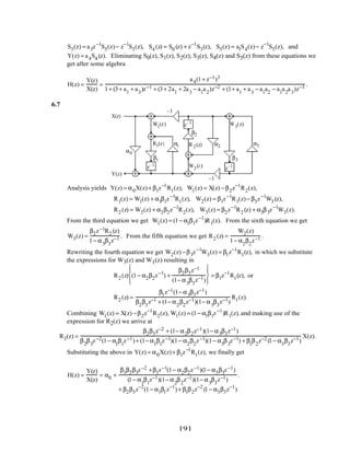
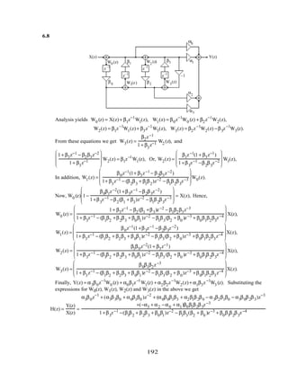
197. 6.9
X(z) Y(z)
1
1 − z−1
1
1− z
−1
W(z) U(z) −k1
k1 k2
Analysis yields (1): W(z) = X(z) + k1Y(z), (2): U(z) =
1
1− z−1 W(z) + k2Y(z), and
(3): Y(z) =
−k1
1− z−1 U(z). Substituting Eq. (2) in Eq. (3) we get
(4): Y(z) =
−k1
1− z−1
1
1− z−1 W(z) + k2Y(z)





 = −
k1
(1− z−1
)2 W(z) −
k1k2
1− z−1 Y(z). Substituting
Eq. (1) in Eq. (4) we then get Y(z) = −
k1
(1− z−1
)2 X(z) + k1Y(z)[ ]−
k1k2
1− z−1 Y(z)
= −
k1
(1− z−1
)2 X(z) −
k1
1− z−1
k1 + k2 − k2z−1
1− z−1








Y(z), or
1+
k1(k1 + k2 − k2z−1
)
(1− z−1
)2








Y(z) = −
k1
(1 − z−1
)2 X(z). Hence,
H(z) =
Y(z)
X(z)
= −
k1
1+ k1(k1 + k2 )[ ]− (2 + k1k2)z−1
+ z−2 .
6.10 (a) A direct form realization of
H(z) = 1− 3.5z−1
+ 4.9z−2
− 3.43z−3
+1.2005z−4
− 0.16807z−5
and its transposed structure aare
shown below:
z−1
z−1
z−1
z−1
z−1
–3.5 4.9 –3.43 1.2005 –0.16807
x[n]
y[n]
–3.54.9–3.431.2005–0.16807
x[n]
y[n]z −1
z −1
z−1
z−1
z−1
(b) A cascade realization of
H(z) = (1− 0.7z−1
)(1− 0.7z−1
)(1− 0.7z−1
)(1− 0.7z−1
)(1− 0.7z−1
) is shown below:
x[n] y[n]
z−1 z−1
z−1
z−1
z−1
–0.7 –0.7 –0.7 –0.7 –0.7
(c) A cascade realization of H(z) = (1− 0.7z−1
)(1− 1.4z−1
+ 0.49z−2
)(1− 1.4z−1
+ 0.49z−2
) is
shown below:
193

198. x[n] y[n]z−1 z−1 z−1 z −1 z −1
–0.7
–1.4 –1.4
0.49 0.49
(d) A cascade realization of H(z) = (1− 2.1z−1
+ 1.47z−2
− 0.343z−3
)(1 −1.4z−1
+ 0.49 z−2
) is
shown below:
x[n] y[n]z−1
z −1
z −1
z −1 z −1
–1.4
0.49
–2.1 0.98
–0.343
6.11 (a) H(z) = h[0]+ h[3]z−3
+ h[6]z−6
( )+ z−1
h[1] + h[4]z−3
+ h[7]z−6
( )+ z−2
h[2] + h[5]z−3
( ).
Hence, E0(z) = h[0]+ h[3]z−3
+ h[6]z−6
, E1(z) = h[1]+ h[4]z−3
+ h[7]z−6
, E2(z) = h[2]+ h[5]z−3
.
(b)
Figure is same as in Figure 6.9 with h[8] = 0.
6.12 (a) H(z) = h[0]+ h[2]z−2
+ h[4]z−4
+ h[6]z−6
( )+ z−1
h[1] + h[3]z−2
+ h[5]z−4
+ h[7]z−6
( ).
Hence, E0(z) = h[0]+ h[2]z−2
+ h[4]z−4
+ h[6]z−6
, E1(z) = h[1]+ h[3]z−2
+ h[5]z−4
+ h[7]z−6
.
(b)
X(z) Y(z)
h[0]
h[1]
h[2]
h[4] h[6]
h[3]
h[5]
h[7]
z−2
z−2 z−2
z−1
6.13 (a) H(z) = h[0]+ h[4]z−4
( )+ z−1
h[1] + h[5]z−4
( )+ z−2
h[2] + h[6]z−4
( )+ z−3
h[3] + h[7]z−4
( ).
Hence, E0(z) = h[0]+ h[4]z−4
, E1(z) = h[1]+ h[5]z−4
,
E2(z) = h[2]+ h[6]z−4
, E3(z) = h[3]+ h[7]z−4
.
194

199. (b)
z−1
z−1
z−1
z −4
h[0]
h[2]
h[4]
h[6]
h[1]
h[3]
h[5]
h[7]
6.14
x[n]
y[n]
z−1
z−1 z−1
z−1
z−1
z−1
z−1
z−1
−1 −1 −1 −1
h[0] h[1] h[2] h[3]
6.15
x[n]
y[n]
z−1
z−1
z−1
z−1
z−1
z−1
z−1
z−1
−1 −1 −1 −1
h[0] h[1] h[2] h[3]
z−1
h[4]
−1
6.16 Consider first the case of N = 4.
H(z) = b0 + b1z−1
1+ +b2z−1
1+ b3z−1
1+ b4z−1
( )( )( )= b0 + b1z−1
1+ +b2z−1
1+ b3z−1
+ b3b4z−2
( )( )
= b0 + b1z−1
1+ b2z−1
+ b2b3z−2
+ b2b3b4z−3
( )
= b0 + b1z−1
+ b1b2z−2
+ b1b2b3z−3
+ b1b2b3b4z−4
= h[0]+ h[1]z−1
+ h[2]z−2
+ h[3]z−3
+ h[4]z−4
.
Comparing like powers of z−1
on both sides, we obtain h[0]= b0 , h[1] = b1, h[2]= b1b2 ,
h[3] = b1b2b3 , h[4] = b1b2b3b4. Solving these equations we get b0 = h[0], b1 = h[1], b2 =
h[2]
h[1]
,
b3 =
h[3]
h[2]
, and b4 =
h[4]
h[3]
. In the general case, we have
b0 = h[0], b1 = h[1],and bk =
h[k]
h[k −1]
, 2 ≤ k ≤ N.
A nested realization of H(z) for N = 7 is shown below:
195

200. z−1
z−1 z−1
x[n] y[n]
z−1
z−1
z−1
b0
b1 b2 b3 b 4 b5
z−1
b6 b7
6.17 G(z) = z−N / 2
− H(z). A canonic realization of both G(z) and H(z) is as indicated on next page
for N = 8.
z−1
z−1
z−1
z−1 z−1 z−1
z−1
G(z)
H(z)
z−1 −1
h[0] h[1] h[2] h[3] h[4]
6.18 Without any loss of generality, assume M = 5 which means N = 11. In this case the transfer
function is given by H(z) =
z
−5
h[5] + h[4](z + z
−1
) + h[3](z
2
+ z
−2
) + h[2](z
3
+ z
−3
) + h[1](z
4
+ z
−4
) + h[0](z
5
+ z
−5
)[ ].
Now, the recursion relation for the Chebyshev polynomial is given by
Tr (x) = 2xTr−1(x) − Tr−2 (x), for r ≥ 2 with T0 (x) =1 and T1(x) = x. Hence,
T2 (x) = 2xT1(x) − T0 (x) = 2x2
− 1, T3(x) = 2xT2(x) − T1(x) = 2x(2x2
− 1) − x = 4 x3
− 3x,
T4 (x) = 2x T3 (x) − T2 (x) = 2x(4x3
− 3x) − (2x2
−1) = 8x4
− 8x2
+1,
T4 (x) = 2x T3 (x) − T2 (x) = 2x(4x3
− 3x) − (2x2
−1) = 8x4
− 8x2
+1,
We can thus rewrite the expression inside the square brackets given above as
h[5]+ 2h[4]T1
z + z−1
2





 + 2h[3]T2
z + z−1
2





 + 2h[2]T3
z + z−1
2






+2h[1]T4
z + z−1
2





 + h[0]T5
z + z−1
2






= h[5]+ 2h[4]
z + z−1
2





 + 2h[3] 2
z + z−1
2






2
− 1








+ 2h[2] 4
z + z−1
2






3
− 3
z + z−1
2














+ 2h[1] 8
z + z−1
2






4
− 8
z + z−1
2






2
+ 1








+ 2h[0] 16
z + z−1
2






5
− 20
z + z−1
2






3
+ 5
z + z−1
2














196

201. = a[n]
z + z−1
2






n =0
5
∑
n
, where a[0]= h[5] − 2h[3] + 2h[1], a[1]= 2h[4] − 6h[2] +10 h[0],
a[2] = 4h[3] −16 h[1], a[3]= 8h[2] − 40h[1], a[4]= 16h[1], and a[5] = 32 h[0].
A realization of H(z) = z−5
a[n]
z + z−1
2






n=0
5
∑
n







= a[0]z−5
+ a[1]z−4 1+ z−2
2






+ a[2]z−3 1+ z−2
2






2
+a[3]z−2 1+ z−2
2






3
+ a[4]z−1 1 + z−2
2






4
+ a[5]
1+ z−2
2






5
is thus as shown below:
6.19 Consider H(z) =
P(z)
D(z)
=
P1(z)
D1(z)
⋅
P2 (z)
D2(z)
⋅
P3(z)
D3(z)
. Assume all zeros of P(z) and D(z) are complex.
Note that the numerator of the first stage can be one of the 3 factors, P1(z), P2(z), and P3(z), the
numerator of the second stage can be one of the remaining 2 factors, and the numerator of the
third stage is the remaining factor. Likewise, the denominator of the first stage can be one of
the 3 factors, D1(z), D2(z), and D3(z), the denominator of the second stage can be one of the
remaining 2 factors, and the denominator of the third stage is the remaining factor. Hence,
there are (3!)2
= 36 different types of cascade realizations.
If the zeros of P(z) and D(z) are all real, then P(z) has 6 real zeros and D(z) has 6 real zeros. In
this case then there are (6!)2
= 518400 different types of cascade realizations.
6.20 H(z) =
Pi (z)
Di(z)
i=1
K
∏ . Here the numerator of the first stage can be chosen in
K
1





 ways, the
numerator of the second stage can be chosen in
K −1
1





 ways, and until the there is only
possible choice for the numerator of the K-th stage. Likewise, the denominator of the first
stage can be chosen in
K
1





 ways, the denominator of the second stage can be chosen in
K −1
1





 ways, and until the there is only possible choice for the denominator of the K-th stage.
Hence the total number of possible cascade realizations are equal to
K
1






2
K −1
1






2
K − 2
1






2
L
2
1






2
1
1






2
= (K!)2
6.21 A canonic direct form II realization of H(z) =
3+ 4z−1
− 2z−2
1+ 3z−1 + 5z−2 + 4z−4 is shown on next page:
197

202. x[n] y[n]z
–1
z
–1
z
–1
z
–1
z
–1
–3 –5 –4
3
4
–2
A canonic direct form IIt realization of H(z) is as indicated below:
x[n] y[n]z
–1
z
–1
z
–1
z
–1
z
–1
–3–5–4
3
4
–2
6.22 (a) A cascade realization of H1(z) =
0.3− 0.5z−1
1+ 2.1z−1 − 3z−2






2 + 3.1z−1
1+ 0.67 z−1





 is shown below:
x[n] y[n]z
–1
z
–1
z
–1
–2.1 3
0.3 –0.5
–0.67
2
3.1
A cascade realization of H1(z) =
2+ 3.1z−1
1+ 2.1z−1 − 3z−2






0.3− 0.5z−1
1+ 0.67 z−1





 is shown below:
x[n] y[n]z
–1
z
–1
z
–1
–2.1 3
0.3
–0.5
–0.67
2 3.1
(b) A cascade realization of H2(z) =
4.1z (z − 1
3
)
(z + 0.3)(z − 0.5)












z2
+ 0.4
z2 − z − 0.1






=
4.1−1.3667z−1
1− 0.2z−1 − 0.15z−2






1+ 0.4z−2
1− z−1 + 0.1z−2





 is shown below:
z
–1
z
–1x[n] y[n]z
–1
z
–1
4.1 –4.1/3
0.2 0.15
0.4
–0.1
198

203. A cascade realization of H2(z) =
1+ 0.4z−2
1− 0.2z−1 − 0.15 z−2






4.1−1.3667 z−1
1− z−1 + 0.1z−2





 is shown below:
z
–1
z
–1x[n]
y[n]
z
–1
z
–1
4.1 –4.1/3
0.2 0.15
0.4
–0.1
(c) A cascade realization of H3(z) =
3− 2.1z−1
1+ 0.52 z−1






2.7 + 4.2z−1
− 5z−2
1+z−1 − 0.34 z−2





 is shown below:
z
–1x[n] y[n]z
–1
z
–1
–0.52
3
–2.1
2.7 4.2
–5
–1 0.34
A cascade realization of H3(z) =
2.7 + 4.2z−1
− 5z−2
1+ 0.52z−1






3− 2.1z−1
1+ z−1 − 0.34 z−2





 is shown below:
z
–1
z
–1x[n]
y[n]
z
–1
z
–1
–0.52
3 –2.12.7 4.2
–5
–1 0.34
6.23 (a) A partial-fraction expansion of H1(z) in z−1
obtained using the M-file residuez gives
H1(z) =
0.6− 0.07z−1
−1.55z−2
1+ 2.77z−1 −1.593z−2 − 2.01z−3 =
0.4454
1+ 3.0755z−1 −
0.1571
1− 0.9755z−1 +
0.3117
1+ 0.67 z−1 whose
realization yields the Parallel Form I structure shown below:
z
–1
x[n] y[n]
z
–1
z
–1
–3.0755
0.9755
–0.67
0.4454
–0.1571
0.3117
199

204. A partial-fraction expansion of H1(z) in z obtained using the M-file residue gives
H1(z) =
0.6z3
− 0.07z2
−1.55z
z3 + 2.77z2 −1.593z − 2.01
= 0.6 +
−1.3699
z + 3.0755
+
0.1533
z − 0.9755
+
−2088
z + 0.67
= 0.6 +
−1.3699z−1
1+ 3.0755z−1 +
0.1533z−1
1− 0.9755z−1 +
−2088z−1
1+ 0.67 z−1 , whose realization yields the Parallel Form II
structure shown below:
z
–1
x[n] y[n]
z
–1
z
–1
–3.0755
0.9755
–0.67
0.6
–1.3699
–0.1533
–0.2088
(b) A partial-fraction expansion of H2(z) in z−1
obtained using the M-file residuez gives
H2(z) =
4.1z4
− 1.3667z3
+ 1.64 z2
− 0.5467z
z4
−1.2z3
+ 0.15z2
+ 0.13z − 0.015
=
7.5709
1− 0.8873z−1 +
−3.7014
1− 0.5z−1 +
3.2458
1+ 0.3z−1 +
−3.0153
1− 0.1127z−1 whose realization yields the Parallel
Form I structure shown below:
z
−1
z
−1
z−1
z
−1
x[n] y[n]
7.5709
0.8873
–3.7014
0.5
3.2458
–0.3
–3.0153
0.1127
200

205. A partial-fraction expansion of H2(z) in z obtained using the M-file residue gives
H1(z) = 4.1+
6.7176
z − 0.8873
+
−1.8507
z − 0.5
+
−0.9737
z + 0.3
+
−0.3398
z − 0.1127
= 4.1+
6.7176 z−1
1− 0.8873z−1 +
−1.8507 z−1
1− 0.5z−1 +
−0.9737z−1
1+ 0.3z−1 +
−0.3398z−1
1− 0.1127 z−1 whose realization yields the
Parallel Form II structure shown below:
z−1
z−1
z−1
x[n] y[n]
0.8873
0.5
–0.3
0.1127
z−1
4.1
6.7176
–1.8507
–0.9737
–0.3398
(c) A partial-fraction expansion of H3(z) in z−1
obtained using the M-file residuez gives
H3(z) =
8.1+ 6.93z−1
− 23.82z−2
+10.5z−3
1+ 1.52 z−1
+ 0.18z−2
− 0.1768z−3 = −59.3891 +
−24.2434
1 +1.2681z−1 +
77.0449
1+ 0.52z−1 +
14.6876
1− 0.2681z−1
whose realization yields the Parallel Form I structure shown below:
z
−1
z
−1
z
−1
x[n] y[n]
–59.3891
–24.2434
77.0449
14.6876
–1.2681
–0.52
0.2681
201

206. A partial-fraction expansion of H3(z) in z obtained using the M-file residue gives
H3(z) = 8.1+
30.7434
z +1.2681
+
−40.0633
z + 0.52
+
3.938
z − 0.2681
= 8.1+
30.7434z−1
1+1.2681z−1 +
−40.0633z−1
1+ 0.52z−1 +
3.938z−1
1− 0.2681z−1
whose realization yields the Parallel Form II structure shown below:
z
−1
z
−1
z
−1
x[n] y[n]
–1.2681
–0.52
0.2681
8.1
30.7434
–40.0633
3.938
6.24 A cascade realization based on the factorization
H(z) =
z−1
1+ 0.8z−1 + 0.5z−2






0.44 + 0.362z−1
+ 0.02z−2
1− 0.4z−1





 is indicated below:
z
–1x[n] y[n]z
–1
z
–1
z
–1
–0.8 –0.5
0.44 0.362
0.02
0.4
6.25 (a) H(z) =
2 + 0.1z−1
1+ 0.4z−1 ⋅
3+ 0.2z−1
1− 0.3z−1 ⋅
1
1− 0.2z−1 =
6 + 0.7z−1
+ 0.02 z−2
1− 0.1z−1
− 0.14z−2
+ 0.024z−3 .
(b) y[n] = 6x[n]+ 0.7x[n −1]+ 0.02x[n − 2]+ 0.1y[n −1]+ 0.14 y[n− 2]− 0.024y[n − 3].
(c) A cascade realization of H(z) is shown below:
z
−1
z
−1
z
−1x[n] y[n]
2
0.1
–0.4
3
0.2
0.3 0.2
(d) A parallel form I realization of H(z) is obtained by making a partial-fraction expansion in
using M-File residuez H(z) =
1.6667
1+ 0.4z−1 +
11
1− 0.3z−1
−6.6667
1− 0.2z−1 ,
202

207. whose realization is shown below:
z−1
z−1
z−1
x[n] y[n]
–0.4
0.3
0.2
1.6667
11
–6.6667
(e) h[n] =1.6667(−0.4)n
µ[n]+ 11(0.3)n
µ[n]− 6.6667(0.2)n
µ[n].
6.26 (a) Y(z) =
1
1− 0.4z−1 −
0.3z−1
1− 0.4z−1 =
1− 0.3z−1
1− 0.4z−1 . X(z) =
1
1− 0.2z−1 . Thus,
H(z) =
Y(z)
X(z)
=
(1− 0.3z−1
)(1− 0.2z−1
)
1− 0.4z−1 =
1− 0.5z−1
+ 0.06 z−2
1− 0.4z−1 .
(b) y[n] = x[n]− 0.5x[n −1] + 0.06x[n − 2]+ 0.4y[n −1].
(c)
z−1z−1x[n] y[n]
0.4
–0.5
0.06
(d) A partial-fraction expansion of H(z) in z−1
obtained using M-file residuez is given
by H(z) = 0.875z−1
− 0.15 +
0.125
1− 0.4z−1 whose realization yields the Parallel Form I structure as
indicated below:
z
−1
z
−1x[n] y[n]
0.4
0.875
–0.15
0.125
(e) The inverse z-transform of H(z) yields h[n] = 0.875δ[n −1]− 0.15δ[n] + 0.125(0.4)n
µ[n].
203

208. (f) X(z) =
1
1− 0.3z−1 −
0.4z−1
1− 0.3z−1 =
1− 0.4z−1
1− 0.3z−1 . Therefore
Y(z) = H(z)X(z) =
(1− 0.3z−1
)(1− 0.2z−1
)
1− 0.4z−1






1− 0.4z−1
1− 0.3z−1





 = 1− 0.2z−1
, whose inverse
z-transform yields y[n] = δ[n]− 0.2δ[n −1].
6.27 Figure P6.11 can be seen to be a Parallel Form II structure. A partial-fraction expansion of
H(z) =
3z2
+18.5z + 17.5
(z + 0.5)(z + 2)
in z obtained using the M-file residue is given by
H(z) = 3+
5
z + 2
+
6
z + 0.5
. Comparing the coefficients of the expansion with the corresponding
multiplier coefficients in Figure P6.11 we conclude that the multiplier coefficient 2 should be
replaced with 6 and the multiplier coefficient 0.5 should be replaced with – 0.6.
6.28 Figure P6.11 can be seen to be a Parallel Form I structure. A partial-fraction expansion of
H(z) =
3z(5z −1)
(z + 0.5)(4z +1)
=
3.75−1.5z−1
1+ 0.75z−1 + 0.125z−2 in z−1
obtained using the M-file residuez is
given by H(z) =
13.5
1+ 0.5z−1 −
9.5
1+ 0.25z−1 . Comparing the coefficients of the expansion with the
corresponding multiplier coefficients in Figure P6.11 we conclude that the multiplier
coefficient A = 13.5 and the multiplier coefficient B = –0.25.
6.29 The difference equation corresponding to the transfer function H(z) =
Y(z)
X(z)
=
1+ α + β
1+ αz
−1
+β z
−2
is given by y[n]+α y[n −1]+β y[n − 2] = (1+ α + β)x[n], which can be rewritten in the form
y[n]= x[n]+ α(x[n]− y[n −1]) + β(x[n]− y[n − 2]). A realization of H(z) based on this equation is
thus as shown below:
6.30 (a) The difference equation corresponding to the transfer function
H(z) =
Y(z)
X(z)
=
(1+ α1 + α2)(1+ 2z−1
+ z−2
)
1− α1 z
−1
+ α2z
−2 is given by
y[n]+ α1 y[n −1]− α2y[n − 2]= (1+ α1 + α2 )(x[n]+ 2x[n −1]+ x[n − 2]), which can be rewritten as
y[n] = (x[n]+ 2x[n −1]+ x[n − 2]) + α1 (y[n −1]− x[n]− 2x[n −1]− x[n − 2])
−α2 (y[n − 2]− x[n]− 2x[n− 1]− x[n − 2]). Denoting w[n] = x[n]+ 2x[n −1]+ x[n − 2],
the difference equation representation becomes
y[n] = w[n]+ α1(y[n −1]− w[n]) − α2(y[n − 2] − w[n]). A realization of H(z) based on the last two
204

209. equations is as indicated below where the first stage realizes w[n] while the second stage realizes
y[n].
An interchange of the two stages leads to an equivalent realization shown below:
Finally, by delay sharing the above structure reduces to a canonic realization as shown below:
(b) The difference equation corresponding to the transfer function
H(z) =
Y(z)
X(z)
=
(1− α2)(1− z−2
)
1− α1z
−1
+ α2z
−2 is given by
y[n]− α1y[n −1]+ α2y[n − 2]= (1− α2)(x[n]− x[n− 2]) which can be rewritten as
y[n] = α1y[n −1]− α2y[n − 2]+ x[n]− α2x[n]− x[n − 2]− α2x[n − 2]
= α1y[n −1]− α2 (x[n]− x[n − 2]+ y[n − 2]) + (x[n]− x[n − 2]). Denoting w[n] = x[n]− x[n − 2],we
can rewrite the last equation as y[n] = α1y[n −1]− α2 (w[n] + y[n− 2]) + w[n]. A realization of
H(z) based on the last two equations is as shown below:
An interchange of the two stages leads to an equivalent realization shown below:
205

210. Finally, by delay sharing the above structure reduces to a canonic realization as shown below:
6.31 (a) From the structure of Figure P.6/14 it follows that HN(z) =
Y1
X1
=
C + DHN−1
(z)
A + BHN−1(z)
, from
which we get HN−1(z) =
C − AHN(z)
B HN (z)− D
. Substituting the expression for HN(z) we then arrive
at HN−1(z) =
C 1+ diz−i
i=1
N
∑







 − A piz−i
i=0
N
∑








B pi
z−i
i=0
N
∑








− D 1+ di
z−i
i=1
N
∑








=
(C − Ap0 )+ (Cd1 − Ap1)z−1 +L+ +(CdN−1 − ApN−1)z−N +1 + +(CdN − ApN )z−N
(Bp0
− D) +(Bp1
− Dd1
)z−1 +L+ (BpN −1
− DdN−1
)z−N +1 + (BpN
− DdN
)z−N .
Substituting the values A = 1, B = dNz–1, C = p0, and D = pNz–1, we get HN–1(z)
=
(p0 − p0 )+ (p0d1 − p1)z−1 +L+ (p0dN −1 − pN−1)z−N +1 + (p0dN − pN)z−N
(dN
p0
− pN
)z−1 + (dN
p1
− pN
d1
)z−2 +L+ (dN
pN−1
− pN
dN −1
)z−N + (dN
pN
− pN
dN
)z−N−1
=
(p0d1 − p1)+ (p0d2 − p2 )z−1 +L+ (p0dN−1 − pN−1)z−N+2 +(p0dN − pN )z−N+1
(p0
dN
− pN
) + (p1
dN
− pN
d1
)z−1 +L+ (pN −1
dN
− pN
dN −1
)z−N+1
=
p0' +p1' z−1 + L+ pN−2' z−N+2 + pN−1' z−N+1
1+ d1
' z−1 + L+ dN−1
' z−N+1 where
pk' =
pk
dk+1
− pk+1
p0dN − pN
, k = 0,1,K,N −1, and dk' =
pk
dN
− pN
dk
p0dN − pN
, k = 1,2,K,N −1.
(b) From the chain parameters, we obtain for the first stage t11 =
C
A
= p0,
t12 =
AD − BC
A
= (pN − p0dN )z−1
, t21 =
1
A
=1, and t22 = −
B
A
= −dNz−1
. The
corresponding input-output relations are then given by
206

211. Y1 = p0X1 + (pN − p0dN )z−1
= p0(X1 − dN z−1
X2 ) + pNz−1
X2,
Y2 = X1 − dN z−1
X2. Substituting the second equation into the first we rewrite it as
Y1 = p0Y2 + pNz−1
X2. A realization of the two-pair based on the last two equations is
therefore as indicated below:
Except for the first stage, all other stages require 2 multipliers. Hence the total number of
multipliers needed to implement an N-th order transfer function HN(z) is 2N+1. The total
number of two-input adders required is 2N while the overall realization is canonic requiring N
delays.
6.32 From H3(z) =
0.44z−1
+ 0.362z−2
+ 0.02z−3
1+ 0.4z−1
+ 0.18z−2
− 0.2z−3 , using Eq. (6.135) we arrive at
H2(z) =
22 +18.1z
−1
+ z
−2
1+ 4.8z
−1
+ 8.8z
−2 . Repeating the procedure we obtain H1(z) =
1.0593 +z
−1
1+ 0.7746 z
−1 .
From H3(z), H2(z) and H1(z) we then arrive at the cascaded lattice realization of H3(z) as
shown below:
z–1 z–1 z–1
0.2
0.44
0.02
–3.8
22 –0.7746
1.0593
6.33 (a) From H3(z) =
0.6− 0.07z−1
−1.55z−2
1+ 2.77z−1 −1.593z−2 − 2.01z−3 (Note the change in the labelling of the
transfer function) using Eq. (6.135) we arrive at H2(z) =
−1.4362 − 0.4927z−1
+ z−2
1− 0.1167z−1 − 2.5833z−2 .
Repeating the procedure we obtain H1(z) =
0.2436 + z−1
1+ 0.5127z−1 . From H3(z), H2(z) and H1(z) we
then arrive at the cascaded lattice realization of H3(z) as shown below:
z
–1
z
–1
z
–1
2.01
0.6
2.5833
–1.4362
–0.5127
0.2436
x[n]
y[n]
207

212. (b) From H4(z) =
4.1− 1.3667z−1
+ 1.64z−2
− 0.5467z−3
1− 1.2z−1 + 0.15z−2 + 0.13z−3 − 0.015z−4 (Note the change in the labelling
of the transfer function) using Eq. (6.135) we arrive at
H3(z) =
57.7772+ 16.6667z−1
−17.5561z−2
+ z−3
1− 0.3333z−1 + 0.4z−2 − 0.1333z−3 . Repeating the procedure we obtain
H2(z) =
4.1284 − 4.6735z−1
+z−2
1+ 0.2170z−1 − 0.2230z−2 , and H2(z) =
−2.8997+ z−1
1− 0.4296z−1 . From H4(z), H3(z), H2(z)
and H1(z) we then arrive at the cascaded lattice realization of H3(z) as shown below:
z
–1
z
–1
z
–1
x[n]
y[n]
z
–1
0.015
0.6
0.1333
57.7772
0.223
4.1284
0.4296
–2.8997
(c) From H3(z) =
8.1+ 6.93z−1
− 23.82 z−2
+10.5z−3
1+ 1.52z−1 + 0.18z−2 − 0.1768z−3 using Eq. (6.135) we arrive at
H2(z) =
−0.4511− 2.1185z−1
+ z−2
1+1.4403z−1 − 3.3873z−2 . Repeating the procedure we obtain H2(z) =
2.7827 + z−1
1+ 10.866z−1 .
From H3(z), H2(z) and H1(z) we then arrive at the cascaded lattice realization of H3(z) as
shown below:
z
–1
z
–1
z
–1
x[n]
y[n]
0.1768
8.1
3.3873
–0.4511
–10.866
2.7827
6.34 When HN(z) is an allpass transfer function of the form
HN(z) = AN(z) =
dN + dN−1z
–1
+ L+ z
–N
1+ d1z
–1
+L + dNz
–N , then from Eq. (6.135a), the numerator coefficients
of HN–1(z) are given by pk' =
p0dk+1 − pk +1
p0dN − pN
=
dNdk +1 − dN –k –1
dN
2
−1
, and from Eq. (6.135b) the
denominator coefficients of HN–1(z) are given by
d' N−k −1 =
pN−k−1dN − dN−k−1
p0dN − pN
=
dk+1dN − dN– k–1
dN
2
−1
= pk' , implying HN–1(z) is an allpass
transfer function of order N–1. Since here pN = 1 and p0 = dN, the lattice structure of Problem
6.31 then reduces to the lattice structure employed in the Gray-Markel realization procedure.
208

213. 6.35 (a) Consider the realization of Type 1B allpass transfer function. From its transfer parameters
given in Eq. (6.62b) we arrive at Y1 = z
−1
X1 + (1+ z
−1
)X2 = z
−1
(X1 + X2) + X2, and
Y2 = (1− z
−1
)X1 − z
−1
X2 = X1 − z
−1
(X1 + X2 ). A realization of the two-pair based on these two
equations is as shown below which leads to the structure of Figure 6.36(b).
(b) From the transfer parameters of Type 1At allpass given in Eq. (6.62c) we obtain
Y1 = z
−1
X1 + X2, and Y2 = (1− z
−2
)X1 − z
−1
X2 = X1 − z
−1
(z
−1
X1 + X2) = X1 − z
−1
Y1. A
realization of the two-pair based on these two equations is as shown below which leads to the
structure of Figure 6.36(c).
(c) From the transfer parameters of Type 1Bt allpass given in Eq. (6.62d) we obtain
Y1 = z
−1
X1 + (1− z
−1
)X2 = z
−1
(X1 − X2) + X2, and
Y2 = (1+ z
−1
)X1 − z
−1
X2 = X1 + z
−1
(X1 − X2 ). A realization of the two-pair based on these two
equations is as shown below which leads to the structure of Figure 6.36(d).
6.36 (a) A cascade connection of three Type 1A first-order allpass networks is a shown below
which is seen to require 6 delays:
Simple block-diagram manipulations results in the structure shown below:
By delay-sharing between adjacent allpass sections we arrive at the following equivalent
realization requiring now 4 delays.
(b) A cascade connection of three Type 1At first-order allpass networks is a shown below which
is seen to require 6 delays:
209

214. By delay-sharing between adjacent allpass sections we arrive at the following equivalent
realization requiring now 4 delays.
6.37 Analyzing the structucture of Figure P6.14 we obtain
z
–1
X(z) Y(z)
–1
–1
aW(z)
U(z)
(1): W(z) = X(z) − z−1
U(z), (2) U(z) = a W(z) + z−1
U(z), and (3): Y(z) = −W(z) + U(z).
From Eq. (2) we obtain (4): U(z) =
a
1− z−1 W(z). Substituting Eq. (4) in Eq. (3) we get
(5): Y(z) = −
1− a − z−1
1 − z−1





 W(z). Substituting Eq. (4) in Eq. (1) we get
(6): X(z) =
1− z−1
+ az−1
1− z−1





 W(z). From Eqs. (5) and (6) we finally get
H(z) =
Y(z)
X(z)
=
−(1− a) +z−1
1− (1− a)z−1 .
6.38 We realize A2(z) =
d1d2 + d1 z−1
+ z−2
1+ d1 z
−1
+ d1d2 z
−2 in the form of a constrained three-pair as indicated
below:
210

215. t11 t12 t13
t21 t22 t23
t31
t32
t33










X1
X2
X3 Y3
Y2
Y1
d1
–d 2
From the above figure, we have
Y1
Y2
Y3










=
t11
t12
t13
t21 t22 t23
t31 t32 t33










X1
X2
X3










, and X2 = d1 Y2 , X3 = −d2 Y3.
From these equations, after some algebra we get A2(z) =
Y1
X1
=
N(z)
D(z)
, where
D(z) =1− d1 t22 + d2 t33 + d1d2 (t23t32 − t22t33),and
N(z) = t11 − d1 (t11t22 − t12t21)+ d2 (t11t33 − t13t31)
+ d1d2 t21(t12t33 − t13t32 )+ t31(t22t13 − t12t23)+ t11(t23t32 − t22t33){ }.
Comparing trhe denominator of the desired allpass transfer function with D(z) we get
t22 = z
−1
, t33 = 0, t23t32 = z
−2
. Next, comparing trhe numerator of the desired allpass transfer
function with N(z) we get t11 = z
−1
, t12t21 = z
−1
(z
−2
−1), t13t31 = 0, and
t32(t11t23 − t21t13)+ t31(t22t13 − t12t23)= 1. Substituting the appropriate transfer parameters
from the previous equations into the last equation we simplify it to t13 t21t32 + t31t12t23 = z
−4
−1.
Since t13 t31 = 0, either t13 = 0, or t31 = 0. (Both cannot be simultaneously equal to zero, as this
will violate the condition t13 t21t32 + t31t12t23 = z
−4
−1.
Consider the case t13 = 0. Then the equation above reduces to t31t12t23 = z
−4
−1. From this
equation and t23t32 = z
−2
. it follows that
t32 = z
−2
, t23 = 1, t31t12 = z
−4
− 1= (z
−1
− 1)(z
−1
+1)(z
−2
+ 1).
There are four possible realizable sets of values of t21 and t31 satisfying the last equation and
t12t21 = z
−1
(z
−2
−1). These lead to four different realizable transfer matrices for the three-pair:
Type 2A:
z−2
z−2
−1 0
z
−1
z
−1
1
z
−2
+1 z
−2
0










, Type 2B:
z−2
z−1
+1 0
z
−1
(z
−1
−1) z
−1
1
(z−2
+1)(z−1
−1) z−2
0










,
Type 2C:
z−2
z−1
−1 0
z
−1
(z
−1
+1) z
−1
1
(z−2
+1)(z−1
+1) z−2
0










, Type 2D:
z−2
1 0
z
−1
(z
−2
−1) z
−1
1
z−4
−1 z−2
0










.
A realization of each Type 2 allpass structures is obtained by implementing its respective
transfer matrix, and then constraining the Y2 and X2 variables through the multiplier d1 and
211

216. constraining the Y3 and X3 variables through the multiplier –d2 resulting in the four structures
shown in Figure 6.38 of text.
It can be easily shown that the allpass structures obtained for the case t31 = 0 are precisely the
transpose of the structures of Figure 6.38.
6.39 A cascade connection of two Type 2D second-order allpass networks is a shown below which
is seen to require 8 delays:
By delay-sharing between adjacent allpass sections we arrive at the following equivalent
realization requiring now 6 delays.
The minimum number of multipliers needed to implement a cascade of M Type 2D second-
order allpass sections is thus 4 + 2(M–1) = 2(M + 1).
6.40 We realize A2(z) =
d2 + d1 z−1
+ z−2
1+ d1 z
−1
+ d2 z
−2 in the form of a constrained three-pair as indicated in
the figure in the solution of Problem 6.46. Comparing the numerator and the denominator of
the Type 3 allpass transfer function with N(z) and D(z) given in the solution of Problem 6.46
we arrive at t11 = z
−2
, t22 = z
−1
, t33 = z
−2
, t23t32 = z
−2
, t23t32 = z
−1
(z
−2
− 1),
t13t31 = z
−4
−1, t13t21t32 + t13t21t32 = z
−3
(z
−2
−1) + z
−1
(z
−4
−1). To solve the last four
equations, we preselect t23 and t32 satiasfying t23t32 = z
−2
,and then determine realizable values
for t12, t21, t13, and t31,
212

217. Choice #1: t23 = z–1, t32 = z–2. This leads to four possible realizable sets of values of t12, t21,
t13, and t31, satisfying the constraint equations given earlier and resulting in the transfer
matrices given below:
Type 3A:
z
−2
z
−2
−1 z
−2
− 1
z
−1
z
−1
z
−1
z
−2
+1 z
−2
z
−2










, Type 3B:
z
−2
z
−1
+1 z
−1
+1
z
−1
(z
−1
–1) z
−1
z
−1
(z−1
−1)(z−2
+1) z−2
z−2










,
Type 3C:
z
−2
z
−1
−1 z
−1
−1
z
−1
(z
−1
+1) z
−1
z
−1
(z−1
+1)(z−2
+1) z−2
z−2










, Type 3D:
z
−2
1 1
z
−1
(z
−2
−1) z
−1
z
−1
z−4
−1 z−2
z−2










.
A realization of each Type 3 allpass structures is obtained by implementing its respective
transfer matrix, and then constraining the Y2 and X2 variables through the multiplier d1 and
constraining the Y3 and X3 variables through the multiplier –d2. Realizations of Types 3A, 3C
and 3D allpass are shown in Figure 6.38 of text. The realization of Type 3B allpass is shown
below:
Choice #2: t23 = 1, t32 = z–3. This leads to four possible realizable sets of values of t12, t21,
t13, and t31, satisfying the constraint equations given earlier and resulting in the transfer
matrices given below:
Type 3E:
z
−2
z
−1
(z
−2
−1) z
−2
−1
1 z
−1
1
z
−2
+1 z
−3
z
−2












,Type 3F:
z
−2
z
−1
(z
−1
+ 1) z
−1
+1
z
−1
−1 z
−1
1
(z
−1
−1)(z
−2
+1) z
−3
z
−2












,
Type 3G:
z
−2
z
−1
(z
−1
− 1) z
−1
−1
z
−1
+1 z
−1
1
(z
−1
+1)(z
−2
+1) z
−3
z
−2












, Type 3H:
z
−2
z
−1
(z
−1
−1) z
−1
− 1
z
−2
−1 z
−1
1
z
−4
−1 z
−3
z
−2












.
Realization of Types 3H is shown in Figure 6.38 of text. The realizations of Types 3E, 3F and
3G allpass are shown below:
Choice #3: t23 = z–2, t32 = z–1. The structures in this case are the transpose of the Types
3A, 3B, 3C and 3D allpass networks of Choice #1 given above.
Choice #4: t23 = z–3, t32 = 1. The structures in this case are the transpose of the Types
3E, 3F, 3G and 3H allpass networks of Choice #2 given above.
6.41 A cascade connection of two Type 3H second-order allpass networks is a shown below which
is seen to require 8 delays:
213

218. By delay-sharing between adjacent allpass sections we arrive at the following equivalent
realization requiring now 7 delays.
The minimum number of multipliers needed to implement a cascade of M Type 3H second-
order allpass sections is thus 4 + 3(M–1) = 3M + 1.
6.42 From the transfer parameters given in Eq. (6.52d) we arrive at the input-output relations of the
two-pair as (1): Y1 = kmX1 + z−1
X2 , and (2) Y2 = (1− km
2
)X1 − kmz−1
X2. A three-multiplier
realization based on these two equations is shown below:
z
–1
X1
X2
Y2
Y1
− km
km
1 −km
2
6.43 Eq. (2) in the solution given above can be rewritten as
Y2 = X1 − km
2
X1 − kmz−1
X2 = X1 − km (kmX1 + z−1
X2 ). Substituting Eq. (1) of the solution
given above in this equation we then get (3): Y2 = X1 − km
2
X1 − kmz−1
X2 = X1 − kmY1.
A realization based on Eq. (3) and Eq. (1) in the solution given above results in the lattice
structure shown below:
214

219. z
–1
X1
X2
Y2
Y1
− km
km
Analyzing the above structure we obtain Y1 = kmX1 + z
−1
X2, and
Y2 = X1 − kmY1 = X1 − km kmX1 + z
−1
X2( )= (1 − km
2
)X1 − kmz
−1
X2. Hence, the transfer
parameters of the lattice two-pair are given by
t11 = km, t12 = z
−1
, t21 = 1 − km
2
, t22 = −kmz
−1
.
The corresponding chain parameters are obtained using Eq. (4.176b) and are given by
A =
1
1− km
2
, B =
kmz
−1
1− km
2
, C =
km
1− km
2
, D =
z
−1
1− km
2
.
X1
Y1
W1
S1
− k1
k1
− k2
k2
z
−1 z
−1
Hence, the input-output relation of the all-pole cascaded lattice structure given above can be
expressed as:
X1(z)
Y1(z)





 =
1
(1 − k2
2
)(1− k1
2
)
1 k2z−1
k2 z−1








1 k1z−1
k1 z−1








W1(z)
S1(z)





, from which we
obtain Hr(z) =
W1(z)
X1(z)
=
(1 − k2
2
)(1 − k1
2
)
1 + k1(1+ k2 )z−1
+ k2z−2
.
X1
Y1
W1
S1
− k1
k1
− k2
k2
z
−1
z
−1
Likewise, from Section 6.8.1, we arrive at the input-output relation of the all-pole cascaded
lattice structure given above as:
X1(z)
Y1(z)





 =
1 k2z−1
k2 z−1








1 k1z−1
k1 z−1








W1(z)
S1(z)





, from which we
obtain Hs(z) =
W1(z)
X1(z)
=
1
1+ k1(1 + k2) z−1
+ k2z−2
.
Now for a second-order all-pole transfer function can also be expressed in terms of its poles as
H(z) =
1
1 − 2 rcosωoz−1
+ r2
z−2
. Comparing the denominator of H(z) with that of Hs(z)
215

220. and Hr(z) we observe k2 = r
2
and k1(1 + k2) = −2 r cosωo. As r ≅ 1,
k1 = −
2r cosωo
1+ r2
= −cosωo.
At the true resonance peak, we have H(e
jωr
) =
1
(1 − r2
) sinωo
. Likewise, at ω = ωr ,
Hs(e
jωr
) =
1
(1 − k2) 1 − k1
2
. As r → 1, k2 = r
2
→ 1, and hence, the gain Hs(e
jωr
)
becomes excessively large. In the case of the all-pole structure realized using the reverse lattice
two-pairs, as r → 1, k2 = r
2
→ 1,
(1 − k1
2
)(1 − k2
2
) = (1 − k1
2
)(1 − k2)(1+ k2 ) ≅ 2(1 − k1
2
)(1− k2 ). Hence, at ω = ωr ,
Hr(e
jωr
) ≅
2(1− k1
2
)(1− k2)
(1 − k2) 1 − k1
2
= 2 1− k1
2
= 2 sin ωo . This indicates that the gain at the
peak resonance is approximately independent of the pole radius as long as the pole angle is
constant and the radius is close to 1.
6.44 (a) H1(z) =
2 + z
−1
+ 2z
−2
1− 0.75z
−1
+ 0.125z
−2 . Choose, A2(z) =
0.125− 0.75z
−1
+ z
−2
1− 0.75z
−1
+ 0.125z
−2 . Note
k2 = A2 (∞) = d2 = 0.125 <1. Using Eq. (6.71) we next determine the coefficients of A1(z)
arriving at A1(z) =
0.66667+ z
−1
1− 0.66667z
−1 . Here, k1 = A1(∞) = d1' = −0.66667, Hence,
k1 = 0.66667< 1. Therefore, A2(z) and hence H1(z) is stable.
To determine the feed-forward coefficients we use α1 = p2 = 2, α2 = p1 − α1d1 = 2.5,
α3 = p0 − α1d2 − α2d1' = 3.41667. Final realization of H1(z) is thus as shown below:
X1
Yo
z
–1
z
–1
–0.125
0.125 –0.66667
0.66667
2 2.5 3.41667
(b) H2(z) =
1+ 2z
−1
+ 3z
−2
1− z
−1
+ 0.25z
−2 . Thus, A2(z) =
0.25 −z
−1
+z
−2
1− z
−1
+ 0.25z
−2 . Note k2 = A2 (∞) = d2 = 0.25 < 1.
Using Eq. (6.71) we next determine the coefficients of A1(z) arriving at A1(z) =
–0.8 +z
−1
1− 0.8z
−1 .
Here, k1 = A1(∞) = −0.8. Thus, k1 = 0.8< 1. Therefore, A2(z) and hence H2(z) is stable.
216

221. To determine the feed-forward coefficients we use α1 = p2 = 3, α2 = p1 − α1d1 = 5,
α3 = p0 − α1d2 − α2k1 = 4.25. Final realization of H2(z) is thus as shown below:
X1
Yo
z –1
z
–1
–0.25
0.25 –0.8
0.8
3 5 4.25
(c) H3(z) =
2+ 5z
−1
+ 8z
−2
+ 3z
−3
1+ 0.75z
−1
+ 0.5z
−2
+ 0.25z
−3 . This implies, A3(z) =
0.25+ 0.5z
−1
+ 0.75z
−2
+ z
−3
1+ 0.75z
−1
+ 0.5z
−2
+ 0.25z
−3 .
Note k3 = A3(∞) = d3 = 0.25 <1. Using Eq. (6.71) we next determine the coefficients of A2(z)
arriving at A2(z) =
1
3
+
2
3
z
−1
+z
−2
1+
2
3
z−1
+
1
3
z−2
. Note k2 = A2 (∞) = d2' = 1/3 <1. Using Eq. (6.71) we
next determine the coefficients of A1(z) arriving at A1(z) =
0.5 +z
−1
1+ 0.5z
−1 . Thus,
k1 = A1(∞) = d1"= 0.5 <1. Since ki < 1 for i = 3, 2, 1, A3(z) and hence H3(z) is stable.
To determine the feed-forward coefficients we make use of Eq. (6.98) and obtain α1 = p3 = 3,
α2 = p2 − α1d1 = 5.75, α3 = p1 − α1d2 − α2d1' = −
1
3
. α4 = p0 − α1d3 − α2d2' −α3d1"= −
1
2
.
Final realization of H3(z) is thus as shown below:
z–1
z–1
z–1
X1
Yo
0.25
–0.25 –1/3
1/3
–0.5
0.5
3 5.75 –1/3 –1/2
(d) H4(z) =
1+1.6z
−1
+ 0.6z
−2
1− z
−1
− 0.25z
−2
+ 0.25z
−3 . This implies A3(z) =
0.25 − 0.25z
−1
−z
−2
+ z
−3
1− z
−1
− 0.25z
−2
+ 0.25z
−3 . Note
k3 = A3(∞) = d3 = 0.25 <1. Using Eq. (6.71) we next determine the coefficients of A2(z)
arriving at A2(z) =
−1+ z
−1
1−z
−1 . Note k2 = A2 (∞) = d2' = 0. Using Eq. (6.71) we next determine
the coefficients of A1(z) arriving at A1(z) =
−1+z
−1
1− z
−1 . k1 = A1(∞) = d1"= −1. Since
k1 = 1,A3(z) and hence H4(z) is unstable. Feed-forward coefficients are next determined using
217

222. Eq. (6.98) and are given by α1 = 0, α2 = 0.6, α3 = 2.2, α4 = 3.2. Final realization of H4(z) is
thus as shown below:
X1
Yo
z
–1
z
–1
z
–1
–0.25
–1
0.6 2.2 3.2
(e) H5(z) =
3 +1.5z
−1
+ z
−2
+ 0.5z
−3
1−1.8333z
−1
+1.5z
−2
− 0.5833z
−3
+ 0.0833z
−4 . Hence,
A4(z) =
0.0833− 0.5833z
−1
+1.5z
−2
−1.8333z
−3
+ z
−4
1−1.8333z
−1
+1.5z
−2
− 0.5833z
−3
+ 0.0833z
−4 . Note k4 = A4 (∞) = d4 = 0.0833 < 1.
Using Eq. (6.71) we next determine the coefficients of A3(z) arriving at
A3(z) =
0.433595 +1.38466z
−1
−1.7972z
−2
+z
−3
1−1.7972 z
−1
+1.38466z
−2
− 0.433595z
−3 . Thus, k3 = A3(∞) = d3' = 0.433595 <1.
Continuing this process we obtain A2(z) =
0.74558−1.4739 z
−1
+ z
−2
1− 1.4739z
−1
+ 0.74558z
−2 . Thus,
k2 = A2 (∞) = d2' = 0.74558 <1. Finally we arrive at A1(z) =
−0.84436+ z
−1
1− 0.84436z
−1 . This implies
k1 = A1(∞) = d1'' ' = −0.84436. Since ki < 1 for i = 4, 3, 2, 1, A4(z) and hence H5(z) is stable.
Feed-forward coefficients are next determined using Eq. (6.98) and are given by
α1 = 0, α2 = 0.5, α3 = 1.89859, α4 = 3.606, α5 = 4.846.
6.45 (a) H1(z) =
0.6− 0.07z−1
−1.55z−2
1+ 2.77z−1 −1.593z−2 − 2.01z−3 . Hence
A3(z) =
−2.01−1.593z−1
+ 2.77 z−2
+ z−3
1+ 2.77z−1 − 1.593z−2 − 2.01z−3 . Note k3 = A3(∞) = −2.01. Using Eq. (6.47) we
then arrive at A2(z) =
−1.3074 + 0.1421z−1
+z−2
1+ 0.1421z−1 −1.3074z−2 . Note k2 = A2 (∞) = −1.3074. Using Eq.
(6.47) again we next arrive at A1(z) =
−2.0434 +z−1
1− 2.0434z−1 . Note k1 = A1(∞) = −2.0434. Since
ki > 1, 1≤ i ≤ 3, A3(z) and hence, H1(z) is an unstable transfer function. Next using Eq.
(6.79) we arrive at the feed-forward multipliers: α1 = 0, α2 = −1.55, α3 = 0.1503, and
α4 = 0.4306.
Note that if Program 6_4 is used to realize H1(z) , the following error
message will appear: ??? Error using ==> tf2latc
The IIR system is unstable
218

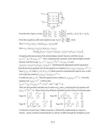
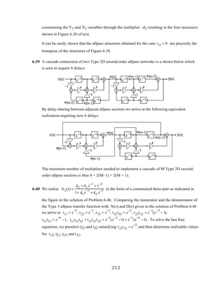
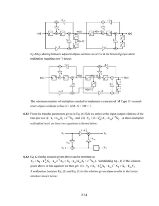
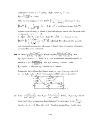
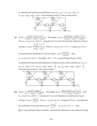
223. z
−1
z
−1
z
−1
x[n]
y[n]
2.01 1.3074
–1.3074 –2.0434
2.0434
–1.55 0.1503 0.4306
(b) H2(z) =
4.1− 1.3667z−1
+ 1.64z−3
− 0.5467z−4
1−1.2z−1 + 0.15 z−2 + 0.13z−3 − 0.015z−4 . Hence,
A4(z) =
−0.015+ 0.13z−1
+ 0.15z−2
−1.2z−3
+ z−4
1−1.2z−1 + 0.15z−2 + 0.13z−3 − 0.015z−4 . Note A4(∞) = k4 = −0.015. Using Eq.
(6.47) we then arrive at A3(z) =
0.112 + 0.1523z−1
−1.1983z−2
+z−3
1−1.1983z−1 + 0.1523z−2 + 0.112z−3 . Note
A3(∞) = k3 = 0.112. Using Eq. (6.47) again we next arrive at
A2(z) =
0.2902 −1.2308z−1
+ z−2
1− 1.2308z−1 + 0.2902z−2 . Note A2(∞) = k2 = 0.2902 . Using Eq. (6.47) we
finally arrive at A1(z) =
−0.9540+ z−1
1− 0.9540 z−1 . Note A1(∞) = k1 = −0.9540. Since ki < 1,
1≤ ki ≤ 4, A4(z) and hence, H2(z) is a stable transfer function.
The feed-forward multipliers αi{ } are determined using the following equations:
α1 = p4 = −0.5467, α2 = p3 − α1d1 = 0.9840, α3 = p2 − α1d2 − α2d1
'
= 1.2611,
α4 = p1 − α1d3 − α2d2
'
−α2d3
"
= 0.1067, and α5 = p0 − α1d4 − α2d3
'
− α2d2
"
− α3d1
"'
= 3.7175,
The lattice and feed-forward multipliers can also be obtained using Program 6_4 yielding
Lattice parameters are
-0.9540 0.2902 0.1120 -0.0150
Feedforward multipliers are
3.7175 0.1067 1.2611 0.9840 -0.5467
z
−1
z
−1
z
−1
x[n]
y[n]
z
−1
–0.015
0.015
0.112
–0.112
0.2902
–0.2902
–0.954
0.954
–0.5467 0.984 1.2611 0.1067 3.7175
219

224. (c) H3(z) =
8.1+ 6.93z−1
− 23.82 z−2
+10.5z−3
1+ 1.52z−1 + 0.18z−2 − 0.1768z−3 . Hence,
A3(z) =
−0.1768+ 0.18z−1
+1.52z−2
+ z−3
1+1.52z−1 + 0.18z−2 − 0.1768 z−3 . Note A3(∞) = k3 = −0.1768 . Using Eq. (6.47)
we then arrive at A2(z) =
0.4632 +1.6019 z−1
+ z−2
1+ 1.6019z−1 + 0.4632z−2 . Note A2(∞) = k2 = 0.4632 . Using Eq.
(6.47) again we next arrive at A1(z) =
1.0948 + z−1
1+1.0948 z−1 . Note A1(∞) = k1 = 1.0948 . Since
k1 >1, A3(z), and hence, H3(z) are unstable transfer functions. Next using Eq. (6.79) we
arrive at the feed-forward multipliers: α1 = 10.5, α2 = −39.78, α3 = 68.7636, and
α4 = −46.8999.
Note that if Program 6_4 is used to realize H3(z), the following error message will appear:
??? Error using ==> tf2latc
The IIR system is unstable
z
−1
z
−1
x[n]
y[n]
z
−1
–0.1768
0.1768
0.4632
–0.4632
1.0948
–1.0948
10.5 –39.78 68.7636 –46.8999
6.52 H(z) =
0.5634(1+ z−1
)(1−1.10166z−1
+z−2
)
(1− 0.683z−1)(1−1.4461z−1 + 0.7957z−2)
.
(a) Direct canonic form - H(z) =
0.05634(1− 0.10166z−1
− 0.10166z−2
+ z−3
)
1− 2.1291z−1 +1.78339z−2 − 0.54346z−3 .
X(z) Y(z)
z–1
z–1
z–1
2.1291
– 1.7833863
– 0.5434631
– 0.10166
– 0.10166
Hardware requirements: # of multipliers = 5, # of two-input adders = 6, # of delays = 3.
(b) Cascade Form
220

225. X(z) Y(z)
z–1
z–1
z
–1
0.683 1.4461
– 0.7957
– 1.0166
0.05634
Hardware requirements: # of multipliers = 5, # of two-input adders = 6, # of delays = 3.
(c) Gray-Markel Form -
z
–1
z
–1
z
–1
X1
α1 α2
α3 α4
Yo
− d3
d3
− d1"
d1"
− d2'
d
2
'
0.05634
d3 = −0.5434631, d2
'
= 0.8881135, d1
"
= − 0.8714813.
α1 = p3 = 1, α2 = p2 − α1d1 = 2.02744, α3 = p1 − α1d2 − α2d1
'
= 1.45224,
α4 = p0 − α1d3 − α2d2
'
− α3d1
"
= 1.00702.
Hardware requirements: # of multipliers = 9, # of two-input adders = 6, # of delays = 3.
(d) Cascaded Lattice Structure -
Using Eqn. (6.152) we obtain H2(z) =
p0
' + p1
' z−1 + p2
' z−2
1+ d1
' z−1 + d2
' z−2 =
1.3136 −1.2213z−1
+ z−2
1−1.4152 z−1 +1.1197z−2 .
and H1(z) =
p0
" + p1
"z−1
1+ d1
"z−1 =
–1.3546 +z−1
1− 0.1015z−1 . The final structure is as shown below:
X1
Yo z
–1
z
–1
z
–1
p0
p3
–d3 −d1"− d2'
p0' p0
"
where p0 = 0.5634, d3 = −0.54346, p3 = 0.5634, p0
'
=1.3136, d2
'
=1.1197,
p0
"
= –1.3546, and d1
"
= – 0.1015.
6.47 (a) A partial fraction expansion of G(z) is of the form G(z) = d +
υi
z − λii=1
N /2
∑ +
υi
*
z − λi
*
i =1
N / 2
∑ . If we
define H(z) =
d
2
+
υi
z − λii=1
N / 2
∑ , then we can write G(z) = H(z) + H*(z), where H*(z) represents the
transfer function obtained from H(z) by conjugating its coefficients.
221

226. (b) In this case, the partial fraction expansion of G(z) is of the form
G(z) = d +
ρi
z − ξi
+
i=1
Nr
∑
υi
z − λii=1
N c
/ 2
∑ +
υi
*
z − λi
*
i=1
Nc
/ 2
∑ , where Nr and Nc are the number of real poles
ξi 's and complex poles λi 's, respectively, with residues ρi 's and υi 's. We can thus decompose
G(z) as G(z) = H(z) + H*(z), where H(z) =
d
2
+
ρi / 2
z − ξi
+
i=1
Nr
∑
υi
z − λii=1
N c
/ 2
∑ .
(c) An implementation of real coefficient G(z) is thus simply a parallel connection of two
complex filters characterized by transfer functions H(z) and H*(z) as indicated in the figure
below:
H(z)
H (z)
*
x[n]
y[n]
= 0
However, for a real valued input x[n], the output of H(z) is the complex conjugate of H*(z). As
a result, two times the real part of the output of H(z) is the desired real-valued sequence y[n]
indicating that single complex filter H(z) is sufficient to realize G(z) as indicated below:
H(z)x[n]
y[n]
2
6.48 From H(z) =
Y(z)
X(z)
=
A + jB
1+ (α + β)z
−1 , we arrive at the difference equation representation
yre[n]+ jyim[n]= –(α + jβ) yre[n− 1]+ jyim[n−1]( )+ Ax[n]+ jB x[n], which is equivalent to a set
of two difference equations involving all real variables and real multiplier coefficients:
yre[n]= –α yre[n−1]+β yim[n −1]+ A x[n], and yim [n] = –βyre[n− 1]– αyim[n −1]+ B x[n].
A realization of H(z) based on the last two equations is shown below:
z–1
z–1
x[n] yre[n]
yim[n]
–α
–α
–β
β
A
B
To determine the transfer function Yre(z)/X(z), we take the z-transforms of the last two
difference equations and arrive at (1+α z
−1
)Yre(z) –β z
−1
Yim(z) = AX(z), and
222

227. βz
−1
Yre(z)+ (1+ αz
−1
)Yim(z) = BX(z). Solving these two equations we get
Yre(z)
X(z)
=
A + (Aα + Bβ)z
−1
1+ 2α z
−1
+ (α
2
+ β
2
)z
−2 , which is seen to be a second-order transfer function.
6.49 An m-th order complex allpass function is given by
Am(z) =
αm
*
+ αm−1
*
z−1
+L+ α1
*
z−(m−1)
+ αm
*
z−m
1+ α1z
−1
+ α2z
−2
+L + αm−1z
−(m−1)
+ αmz
−m .
To generate an (m–1)-th order allpass we use the recursion
Am−1(z) =
Pm−1(z)
Dm−1(z)
= z
Am(z)− km
*
1− kmAm(z)







.
Substituting the expression for Am(z) in the above we obtain after some algebra
Pm−1(z) = z[αm
*
+ αm−1
*
z
−1
+ αm−2
*
z
−2
+L+ α1
*
z
−(m−1)
+ z
−m
− αm
*
(1+ α1z
−1
+ α2z
−2
+L + αm−1z
−(m−1)
+ αmz
−m
)]
= (αm−1
*
− αm
*
α1)+ (αm−2
*
− αm
*
α2)z
−1
+L+ (α1
*
− αm
*
αm−1)z
−(m−2)
+ (1− αm
2
)z
−(m−1)
,
Dm−1(z) = 1+ α1z
−1
+ α2z
−2
+ L+ +αm−1z
−(m−1)
+ αmz
−m
−αm(αm
*
+ αm−1
*
z
−1
+ αm−2
*
z
−2
+L+ +α1
*
z
−(m−1)
+ z
−m
)
= (1− αm
2
)+ (α1 − αmαm−1
*
)z
−1
+ (α2 − αmαm−2
*
)z
−2
+ L+ (αm−1 − αmα1
*
)z
−(m−1)
.
Hence, Am–1(z) is a complex allpass function of order m–1 given by
Am−1(z) =
βm−1
*
+ βm−2
*
z−1
+L +β1
*
z−(m−2)
+ z−(m−1)
1+ β1z
−1
+β2z
−2
+L+ βm−2z
−(m−2)
+βm−1z
−(m−1) ,
where βk =
αk − αmαm−k
*
1− αm
2 , k = 1, 2, . . . , m–1.
To develop a realization of Am(z) we express Am(z) in terms of Am–1(z):
Am(z) =
Y1
X1
=
km
*
− z−1
Am−1(z)
1+ kmz
−1
Am−1(z)
,
and compare it with Eq. (6.73) resulting in the following expressions for the transfer
parameters of the two-pair: t11 = km
*
, t22 = −kmz
−1
, and t12t21 = (1− kmkm
*
)z
−1
. As in the
case of the realization of a real allpass function, there are many possible choices for t12 and t21.
We choose t12 = (1− kmkm
*
)z
−1
, t21 =1. The corresponding input-output relations of the two-
pair Y1 = km
*
X1 + (1− km
*
km )z
−1
X2 = km
*
(X1 − kmz
−1
X2) + z
−1
X2 , and Y2 = X1 − kmz
−1
X2.
A realization of Am(z) based on the above two-pair relations is indicated below:
223

228. Am–1(z)
X1
Y1
– km
z–1
Y2
X2
km
*
Am (z) →
By continuing this process, we arrive at a cascaded lattice realization of a complex allpass
transfer function.
6.50 (a) H1(z) =
2 + 2z
−1
3+ z
−1 =
1
2
1+
1+ 3z
−1
3+ z
−1







 =
1
2
A0(z) + A1(z)( ), where A0(z) = 1 and
A1(z) =
1+ 3z
−1
3+ z
−1 .
(b) H2(z) =
1−z
−1
4+ 2z
−1 =
1
2
1−
2 + 4z
−1
4+ 2z
−1







 =
1
2
A0(z)− A1(z)( ), where A0(z) = 1 and
A1(z) =
2 + 4z
−1
4+ 2z
−1 .
(c) H3(z) =
1− z
−2
4 +2z
−1
+ 2z
−2 =
1
2
1−
2 + 2z
−1
+ 4z
−2
4 + 2z
−1
+ 2z
−2







 =
1
2
A0 (z)− A1(z)( ), where A0(z) = 1
and A1(z) =
2 +2z
−1
+ 4z
−2
4 + 2z
−1
+ 2z
−2 .
(d) H4(z) =
3 + 9z
−1
+ 9z
−2
+ 3z
−3
12 +10z
−1
+ 2z
−2 =
1
2
3+ 9z
−1
+ 9z
−2
+ 3z
−3
(3+ z
−1
)(2 + z
−1
)







 =
1
2
z
−1 1+3z
−1
3+z
−1







 +
1+ 2z
−1
2 +z
−1
















=
1
2
A0(z) + A1(z)( ), where A0(z) = z
−1 1+ 3z
−1
3+ z
−1







 and A1(z) =
1+ 2z
−1
2+ z
−1







 .
6.51 (a) From the equation given we get
y[2l] = h[0]x[2l ]+ h[1]x[2l −1]+ h[2]x[2l − 2]+ h[3]x[2l − 3]+ h[4]x[2l − 4]+ h[5]x[2l − 5], and
y[2l + 1] = h[0]x[2l +1] + h[1]x[2l ]+ h[2]x[2l −1]+ h[3]x[2l − 2] + h[4]x[2l − 3]+ h[5]x[2l − 4].
Rewriting the above two equations in a matrix form we arrive at
y[2l ]
y[2l +1]



 =
h[0] 0
h[1] h[0]




x[2l ]
x[2l +1]



 +
h[2] h[1]
h[3] h[3]




x[2l − 2]
x[2l −1]




+
h[4] h[3]
h[5] h[4]




x[2l − 4]
x[2l − 3]



 +
0 h[5]
0 0




x[2l − 6]
x[2l − 5]



,
which can be alternately expressed as
Yl = H0Xl + H1Xl −1 + H2Xl −2 + H3Xl −3,
224

229. where Yl =
y[2l ]
y[2l +1]



, Xl =
x[2l]
x[2l + 1]



, H0 =
h[0] 0
h[1] h[0]



, H1 =
h[2] h[1]
h[3] h[3]



 ,
H2 =
h[4] h[3]
h[5] h[4]



, and H3 =
0 h[5]
0 0



.
(b) Here y[3l ]= h[0]x[3l]+ h[1]x[3l −1]+ h[2]x[3l − 2]+ h[3]x[3l − 3]+ h[4]x[3l − 4]+ h[5]x[3l − 5],
y[3l +1]= h[0]x[3l + 1]+ h[1]x[3l ]+ h[2]x[3l −1] + h[3]x[3l − 2]+ h[4]x[3l − 3]+ h[5]x[3l − 4], and
y[3l + 2] = h[0]x[3l + 2]+ h[1]x[3l +1]+ h[2]x[3l ]+ h[3]x[3l −1]+ h[4]x[3l − 2] + h[5]x[3l − 3].
Rewriting the above two equations in a matrix form we arrive at
y[3l ]
y[3l +1]
y[3l + 2]








=
h[0] 0 0
h[1] h[0] 0
h[2] h[1] h[0]








x[3l ]
x[3l +1]
x[3l + 2]








+
h[3] h[2] h[1]
h[4] h[3] h[2]
h[5] h[4] h[3]








x[3l − 3]
x[3l − 2]
x[3l − 1]








+
0 h[2] h[1]
0 0 h[2]
0 0 0








x[3l − 6]
x[3l − 5]
x[3l − 4]








,
which can be alternately expressed as Yl = H0Xl + H1Xl −1 + H2Xl −2, where
Yl =
y[3l]
y[3l + 1]
y[3l + 2]








, Xl =
x[3l ]
x[3l +1]
x[3l + 2]








, H0 =
h[0] 0 0
h[1] h[0] 0
h[2] h[1] h[0]








, H1 =
h[3] h[2] h[1]
h[4] h[3] h[2]
h[5] h[4] h[3]








, and
H2 =
0 h[2] h[1]
0 0 h[2]
0 0 0








.
(c) Following a procedure similar to that outlined in Parts (a) and (b) above, we can shw that here
Yl = H0Xl + H1Xl −1 + H2Xl −2, where
Yl =
y[4l ]
y[4l +1]
y[4l + 2]
y[4l + 3]










, Xl =
x[4l]
x[4l + 1]
x[4l + 2]
x[4l + 3]










, H0 =
h[0] 0 0 0
h[1] h[0] 0 0
h[2] h[1] h[0] 0
h[3] h[2] h[1] h[0]










,
H1 =
h[4] h[3] h[2] h[1]
h[5] h[4] h[3] h[2]
0 h[5] h[4] h[3]
0 0 h[5] h[4]










, and H2 =
0 0 0 h[5]
0 0 0 0
0 0 0 0
0 0 0 0










.
6.52 (a) d0 y[2l ]+ d1 y[2l −1]+ d2 y[2l − 2] + d3 y[2l − 3]+ d4 y[2l − 4]
= p0 x[2l] + p1 x[2l −1]+ p2 x[2l − 2]+ p3 x[2l − 3]+ p4 x[2l − 4],
d0 y[2l +1] + d1 y[2l]+ d2 y[2l −1]+ d3 y[2l − 2]+ d4 y[2l − 3]
= p0 x[2l + 1]+ p1 x[2l]+ p2 x[2l −1]+ p3 x[2l − 2] + p4 x[2l − 3],
Rewriting the above two equations in a matrix form we arrive at
d0
0
d1 d0






y[2l]
y[2l +1]



 +
d2 d1
d3 d2






y[2l − 2]
y[2l −1]



 +
d4 d3
0 d4






y[2l − 4]
y[2l − 3]




=
p0
0
p1 p0






x[2l ]
x[2l +1]



 +
p2 p1
p3 p2






x[2l − 2]
x[2l − 1]



 +
p4 p3
0 p4






x[2l − 4]
x[2l − 3]



,
225

230. which can be alternately expressed as D0Yl + D1Yl −1 + D2Yl −2 = P0Xl + P1Xl −1 + P2Xl −1,
where Yl =
y[2l ]
y[2l +1]



, Xl =
x[2l]
x[2l + 1]



, D0 =
d0
0
d1 d0





, D1 =
d2 d1
d3 d2





, D2 =
d4 d3
0 d4





,
P0 =
p0
0
p1 p0





 , P1 =
p2 p1
p3 p2





 , and P2 =
p4 p3
0 p4





 .
(b)
d0
0 0
d1 d0 0
d2 d1 d0










y[3l]
y[3l + 1]
y[3l + 2]








+
d3
d2
d1
d4 d3 d2
0 d4 d3










y[3l − 3]
y[3l − 2]
y[3l −1]








+
0 0 d4
0 0 0
0 0 0








y[3l − 6]
y[3l − 5]
y[3l − 4]








=
p0
0 0
p1 p0 0
p2 p1 p0










x[3l ]
x[3l +1]
x[3l + 2]








+
p3
p2
p1
p4 p3 p2
0 p4 p3










x[3l − 3]
x[3l − 2]
x[3l −1]








+
0 0 p4
0 0 0
0 0 0








x[3l − 6]
x[3l − 5]
x[3l − 4]








,
which can be alternately expressed as D0Yl + D1Yl −1 + D2Yl −2 = P0Xl + P1Xl −1 + P2Xl −1,
where Yl =
y[3l]
y[3l + 1]
y[3l + 2]








, Xl =
x[3l ]
x[3l +1]
x[3l + 2]








, D0 =
d0
0 0
d1 d0 0
d2 d1 d0










, D1 =
d3
d2
d1
d4 d3 d2
0 d4 d3










,
D2 =
0 0 d4
0 0 0
0 0 0







 , P0 =
p0
0 0
p1 p0 0
p2 p1 p0










, P1 =
p3
p2
p1
p4 p3 p2
0 p4 p3










, and P2 =
0 0 p4
0 0 0
0 0 0







 .
(c)
d0 0 0 0
d1
d0
0 0
d2 d1 d0 0
d3
d2
d1
d0












y[4l ]
y[4l +1]
y[4l + 2]
y[4l + 3]










+
d4
d3
d2
d1
0 d4 d3 d2
0 0 d4 d3
0 0 0 d4












y[4l − 4]
y[4l − 3]
y[4l − 2]
y[4l −1]










=
p0 0 0 0
p1
p0
0 0
p2 p1 p0 0
p3
p2
p1
p0












x[4l ]
x[4l +1]
x[4l + 2]
x[4l + 3]










+
p4
p3
p2
p1
0 p4 p3 p2
0 0 p4 p3
0 0 0 p4












x[4l − 4]
x[4l − 3]
x[4l − 2]
x[4l −1]










,
which can be alternately expressed as D0Yl + D1Yl −1 = P0Xl + P1Xl −1, where
Yl =
y[4l ]
y[4l +1]
y[4l + 2]
y[4l + 3]










, Xl =
x[4l]
x[4l + 1]
x[4l + 2]
x[4l + 3]










, D0 =
d0 0 0 0
d1
d0
0 0
d2 d1 d0 0
d3
d2
d1
d0












, D1 =
d4
d3
d2
d1
0 d4 d3 d2
0 0 d4 d3
0 0 0 d4












,
P0 =
p0 0 0 0
p1
p0
0 0
p2 p1 p0 0
p3
p2
p1
p0












, and P1 =
p4
p3
p2
p1
0 p4 p3 p2
0 0 p4 p3
0 0 0 p4












.
6.53 We first rewrite the second-order block-difference equation
D0Yl + D1Yl −1 + D2Yl −2 = P0Xl + P1Xl −1 + P2Xl −1,
as two separate equations: Wl = P0Xl + P1Xl −1 + P2Xl −1, and
Yl = –D0
−1
D1Yl −1 – D0
−1
D2Yl −2 + D0
−1
Wl .
226

231. A cascade realization of the IIR block digital filter based on the above two equations is thus as
shown below:
Wl
YlXl
∆
∆
∆
∆
D0
–1
D
1
D2
P
2
P1
P
0
By interchanging the locations of the two block sections in the above structure we get an
equivalent realization as indicated below:
Yl
Xl
∆
∆
P
2
P1
P0
∆
∆
D
0
–1
D1
D
2
Finally, by delay-sharing the above structure reduces to a canonic realization as shown below:
∆
∆
P
2
P1
P
0
YlXl D
0
–1
D
1
D
2
6.54 By setting αsin θ = ±β in Eq. (6.138), the state-space description of the sine-cosine generator
reduces to
s1[n +1]
s2[n +1]





 =
cosθ ±1
m
β
2
α
2
cosθ










s1[n]
s2[n]





 , which leads to the three-multiplier structure
shown below:
227

232. s2[n]
s1[n]
s1[n +1]s2[n + 1]
z–1 z–1
cosθ cosθ
mβ2
/α2
±1
6.55 By setting α = ±βsinθ in Eq. (6.138), the state-space description of the sine-cosine generator
reduces to
s1[n +1]
s2[n +1]





 = cosθ ±sin
2
θ
m1 cosθ






s1[n]
s2[n]





 , which leads to the three-multiplier structure
shown below:
s2[n]
s1[n]
s1[n + 1]s2[n +1]
z–1 z–1
cosθ cosθ
m1
± sin
2
θ
6.56 Let
β
α
= −
1+ cosθ
sinθ
. Then
α
β
sin θ=
−sin
2
θ
cosθ +1
=
cos
2
θ− 1
cosθ+ 1
= cosθ −1, and, −
β
α
sinθ = cosθ +1.
Substituting these values in Eq. (6.138) we arrive at
s1[n +1]
s2[n +1]





 =
cosθ cosθ −1
cosθ +1 cosθ




s1[n]
s2[n]





 ,
These equations can be alternately rewritten as
s1[n +1]= cosθ s1[n]+ s2[n]( )− s2[n], and s2[n +1] = cosθ s1[n]+ s2[n]( )+ s1[n]. A realization
based on the last two equations results in a single-multiplier structure as indicated below:
s2[n]
s1[n]
s1[n + 1]s2[n + 1]
z–1 z–1
cosθ
–1
6.57
s1[n +1]
s2[n +1]





 =
0
α(C − cosθ)
βsin θ
0 0










s1[n +1]
s2[n +1]





 +
C
α(1− C cosθ)
βsinθ
–
β
α
sinθ cosθ












s1[n]
s2[n]





.
If C = 0, choose α = βsinθ . Then
s1[n +1]
s2[n +1]





 =
0 –cosθ
0 0




s1[n +1]
s2[n +1]





 +
0 1
−1 cosθ




s1[n]
s2[n]





, which can be realized with two
multipliers as shown below:
228

233. s2 [n] s1[n ]s1[n +1]s2 [n +1]
z–1 z–1
cosθ
–cosθ
–1
The above structure can be modified to yield a single multiplier realization as indicated on
next page:
s2[n] s1[n]s1[n +1]s2[n + 1]
z–1 z–1
cosθ
–1
z–1
6.58 If C = 1, then
s1[n +1]
s2[n +1]





 =
0
α(1− cosθ)
βsinθ
0 0










s1[n+1]
s2[n +1]





 +
1
α(1− cosθ)
βsinθ
–
β
α
sinθ cosθ












s1[n]
s2[n]





.
Choose α = βsinθ. This leads to
s1[n +1]
s2[n +1]





 =
0 1− cosθ
0 0




s1[n +1]
s2[n +1]





 +
1 1− cosθ
–1 cosθ




s1[n]
s2[n]





.
A two-multiplier realization of the above equation is shown below:
s2[n] s1[n]s1[n +1]s2[n +1]
z–1 z–1
cosθ
–1
–cosθ1
To arrive at an one-multiplier realization we observe that the two equations describing the sine-
cosine generator are given by s1[n +1]= (1− cosθ)s2[n +1]+ s1[n]+ (1− cosθ)s2[n],and
s2[n +1] = –s1[n]+ cosθs2[n]. Substituting the second equation in the first equation we arrive at
an alternate description in the form
s1[n +1]= –cosθs2[n +1]+ s2[n],
s2[n +1] = –s1[n]+ cosθs2[n].
A realization of above is identical to the single-multiplier structure of Problem 6.64,
6.59 From Figure P6.17(a), the output-input relation of the channel is given by
229

234. Y1(z)
Y2(z)





 =
1 H12(z)
H21(z) 1






X1(z)
X2(z)





.
Likewise, the output-input relation of the channel separation circuit of Figure P6.17(b) is given
by
V1(z)
V2(z)





 =
1 –G12(z)
–G21(z) 1






Y1(z)
Y2(z)





. Hence, the overall system is characterized by
V1(z)
V2(z)





 =
1 –G12(z)
–G21(z) 1






1 H12(z)
H21(z) 1






X1(z)
X2 (z)





 =
1–H21(z)G12(z) H12(z) − G12(z)
H21(z)− G21(z) 1– H12(z)G21(z)






X1(z)
X2 (z)





.
The cross-talk is eliminated if V1(z) is a function of either X1(z) or X2(z), and similarly, if
V2(z) is a function of either X1(z) or X2(z), From the above equation it follows that if H12(z)
= G12(z), and H21(z) = G21(z), then V1(z) = 1– H21(z)G12(z)( )X1(z), and
V2 (z) = 1– H12(z)G21(z)( )X2(z). Alternately, if G12(z) = H21
−1
(z), and G21(z) = H12
−1
(z), then
V1(z) =
H12(z)H21(z) −1
H21(z)







 X2 (z), and V2 (z) =
H12(z)H21(z)−1
H12(z)







 X1(z).
M6.1 (a) H1(z) = (1− 0.3261z−1
)(1− 3.0666z−1
)(1+ 4.748z−1
+ 7.4388z−2
)
×(1−1.0935z−1
+z−2
)(1+ 0.6383z−1
+ 0.1344z−2
) .
(b) H2(z) = (1+ 3.5585z−1
)(1+ 0.281z−1
)(1− z−1
)(1−1.4078z−1
+ 2.0338 z−2
)
×(1+ 0.2604 z−1
+ z−2
)(1− 0.6922 z−1
+ 0.4917z−2
)
M6.2 (a) G(z) =
1.5(1+ 3z−1
+ 4z−2
)(1+ 0.6667z−1
+ 0.3333z−2
)
(1−z−1 + 0.5z−2 )(1−z−1 + 0.3333z−2)
.
(b) G(z) = Ga(z)Gb(z) where Ga(z) =
1.5(1+ 3z−1
+ 4z−2
)
1− z−1 + 0.5z−2 , and
Gb(z) =
1+ 0.6667z−1
+ 0.3333z−2
1− z−1 + 0.3333z−2 . Alternately, we can write G(z) = Gc(z)Gd(z) where
Gc(z) =
1.5(1+ 0.6667z−1
+ 0.3333z−2
)
1−z−1 + 0.5z−2 , and Gd(z) =
1+ 3z−1
+ 4z−2
1− z−1 + 0.3333z−2 .
(c) Parallel form I is obtained using the M-file residuez resulting in the partial fraction
expansion in z−1
of G(z) given by
G(z) = 12 +
−35.25 − j71.25
1−(0.5 − j0.5)z−1 +
−35.25 + j71.25
1− (0.5+ j0.5)z−1 +
30 + j147.22
1− (0.5− j0.2887)z−1 +
30 − j147.22
1− (0.5+ j0.2887)z−1
= 12 +
−70.5− 36 z−1
1− z−1 + 0.5z−2 +
60 + 55z−1
1− z−1 + 0.3333z−2 .
230

235. Parallel form II is obtained using the M-file residue resulting in the partial fraction
expansion in z of G(z) given by
G(z) = 1.5+
(−53.25 + j18)z−1
1− (0.5+ j0.5)z−1 +
(−53.25 − j18)z−1
1−(0.5− j0.5)z−1 +
(57.50 − j64.9519)z−1
1− (0.5+ j0.2887)z−1 +
(57.50 + j64.9519)z−1
1− (0.5− j0.2887)z−1
= 1.5 +
−106.5z−1
+ 35.25z−2
1− z−1 + 0.5z−2 +
115z−1
− 20 z−2
1−z−1 + 0.333z−2 .
M6.3 (a) H(z) =
2(1− 0.6667z−1
+ 0.3333z−2
)(1+ 0.5z−1
+ 0.25z−2
)
(1− 0.5z−1 + 0.5z−2)(1+z−1 + 0.3333z−2 )
.
(b) H(z) = Ha(z)Hb (z) where Ha(z) =
2(1− 0.6667z−1
+ 0.3333z−2
)
1− 0.5z−1 + 0.5z−2 , and
Hb(z) =
1+ 0.5z−1
+ 0.25z−2
1+z−1 + 0.3333z−2 . Alternately, we can write H(z) = Hc(z)dH(z) where
Hc(z) =
2(1− 0.6667z−1
+ 0.3333z−2
)
1+z−1 + 0.3333z−2 , and Hd(z) =
1+ 0.5z−1
+ 0.25z−2
1− 0.5z−1 + 0.5z−2 .
(c) Parallel form I is obtained using the M-file residuez resulting in the partial fraction
expansion in z−1
of H(z) given by H(z) = 1+
0.1622 − j0.286
1− (0.25 − j0.6614)z−1 +
0.1622 + j0.286
1− (0.25 + j0.6614)z−1
+
0.3378 − j1.2093
1+ (0.5+ j0.2887)z−1 +
0.3378 + j1.2093
1+ (0.5− j0.2887)z−1 = 1+
0.3243 − 0.4595z−1
1− 0.5z−1 + 0.5z−2 +
0.6757 − 0.3604 z−1
1+ z−1 + 0.3333z−2 .
Parallel form II is obtained using the M-file residue resulting in the partial fraction
expansion in z of H(z) given by H(z) = 2+
(−0.5135 + j0.1022)z−1
1− (0.25 + j0.6614)z−1 +
(−0.5135 − j0.1022)z−1
1− (0.25 − j0.6614)z−1
+
(−0.1532 − j1.2795)z−1
1+ (0.5− j0.2887)z−1 +
(−0.1532 + j1.2795)z−1
1+ (0.5+ j 0.2887)z−1
= 2 +
−1.027z−1
+ 0.1216z−2
1− 0.5z−1 + 0.5z−2 +
−0.3063z−1
+ 0.5856z−2
1+ z−1 + 0.3333z−2 .
M6.4 Using Program 6_4 we obtain:
Lattice parameters are
-0.8364 0.7980 -0.5143 0.1667
Feedforward multipliers are
63.6358 170.1598 144.1143 57.0000 12.0000
M6.5 Using Program 6_4 we obtain:
231

236. Lattice parameters are
0.3481 0.1801 0.2571 0.1667
Feedforward multipliers are
12.7136 -3.8223 2.5810 -2.0000 4.0000
M6.6 (a) Using Program 6_6 we obtain the following error message:
??? Error using ==> tf2latc
The FIR system has a zero on the unit circle
(b) Using Program 6_6 we obtain the following error message:
??? Error using ==> tf2latc
The FIR system has a zero on the unit circle
M6.7 (a) Using roots we first determine the poles of the denominator of the lowpass transfer
function G(z) which are then paired using the pole interlacing property resulting in the parallel
allpass decomposition given by
G(z) =
1
2
0.1302 − 0.3486z−1
+ z−2
1− 0.3486z−1 + 0.1302z−2 +
−0.0868 + 0.6216 z−1
− 0.6367z−2
+z−3
1− 0.6367z−1 + 0.6216z−2 − 0.0868z−3








.
(b) Hence, the power-complementary highpass transfer function H(z) is given by
H(z) =
1
2
0.1302 − 0.3486z−1
+ z−2
1− 0.3486z−1 + 0.1302z−2 −
−0.0868 + 0.6216 z−1
− 0.6367z−2
+z−3
1− 0.6367z−1 + 0.6216z−2 − 0.0868z−3








=
0.1085(1− 4.9928z−1
+ 9.9891z−2
− 9.9891z−3
+ 4.9928z−4
+ z−5
)
1− 0.9853z−1 + 0.9738z−2 − 0.3864z−3 + 0.1112 z−4 − 0.0113z−5 .
(c)
0 0.2 0.4 0.6 0.8 1
0
0.2
0.4
0.6
0.8
1
ω/π
|H(ejω
)|2
|G(ejω
)|2
|H(ejω
)|2
+ |G(ejω
)|2
232

237. M6.8 (a) Using roots we first determine the poles of the denominator of the highpass transfer
function G(z) which are then paired using the pole interlacing property resulting in the parallel
allpass decomposition given by
G(z) =
1
2
0.5776 + 0.6976 z−1
+ z−2
1+ 0.6976z−1 + 0.5776z−2 −
0.3974 +1.1635z−1
+ 1.0052z−2
+ z−3
1+1.0052z−1 + 1.1635z−2 + 0.3974 z−3








.
(b) Hence, the power-complementary lowpass transfer function H(z) is given by
H(z) =
1
2
0.5776 + 0.6976z−1
+ z−2
1+ 0.6976z−1 + 0.5776z−2 +
0.3974 +1.1635z−1
+1.0052z−2
+z−3
1+1.0052z−1 +1.1635z−2 + 0.3974z−3








=
0.4875(1+ 1.3594z−1
+ 2.2098z−2
+ 2.2098 z−3
+1.3594z−4
+ z−5
)
1+ 1.7028z−1 + 2.4423z−2 +1.7896 z−3 + 0.9492z−4 + 0.2295z−5 .
(c)
0 0.2 0.4 0.6 0.8 1
0
0.2
0.4
0.6
0.8
1
ω/π
|H(e
jω
)|
2
|G(e
jω
)|
2
|G(ejω
)|2
+ |H(ejω
)|2
M6.9 (a) Using roots we first determine the poles of the denominator of the bandpass transfer
function G(z) which are then paired using the pole interlacing property resulting in the parallel
allpass decomposition given by
G(z) =
1
2
0.5874 − 0.5154 z−1
+ z−2
1− 0.5154z−1 + 0.5874 z−2 −
0.6159 + 0.7531z−1
+ z−2
1+ 0.7531z−1 + 0.6159 z−2








(b) Hence, the power-complementary bandstop transfer function H(z) is given by
H(z) =
1
2
0.5874 − 0.5154 z−1
+ z−2
1− 0.5154z−1 + 0.5874 z−2 +
0.6159 + 0.7531z−1
+ z−2
1+ 0.7531z−1 + 0.6159 z−2








= 1.2033
1+ 0.3013z−1
+1.6183z−2
+ 0.3013z−3
+ z−4
1+ 0.2377z−1 + 0.8152 z−2 + 0.1294 z−3 + 0.3618z−4





 .
233

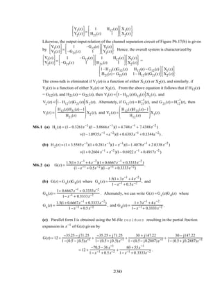
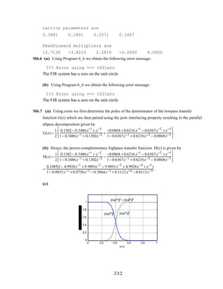
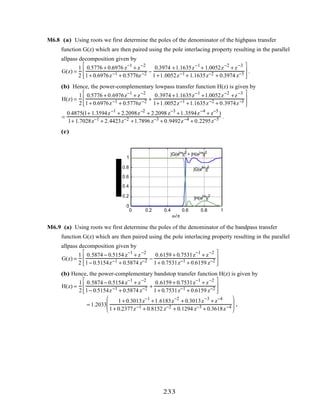
238. (c)
0 0.2 0.4 0.6 0.8 1
0
0.2
0.4
0.6
0.8
1
ω/π
|G(e
jω
)|
2
|H(e
jω
)|
2
|G(e
jω
)|
2
+ |H(e
jω
)|
2
M6.10 The MATLAB program for the simulation of the sine-cosine generator of Problem 6.56 is
given below:
s10 = 0.1; s20 = 0.1; a = 0.9;
y1 = zeros(1,50);y2 = y1;
for n = 1:50;
y1(n) = a*(s10 + s20) - s20;y2(n) = a*(s10 + s20) + s10;
s10 = y1(n);s20 = y2(n);
end
k = 1:1:50;
stem(k-1,y1/abs(y1(7)));axis([0 50 -1.1 1.1]);
xlabel('Time index n');ylabel('Amplitude');
pause
stem(k-1,y2/y2(3));axis([0 50 -1.1 1.1]);
xlabel('Time index n');ylabel('Amplitude');
The plots generated by the above program for initial conditions s1[–1] = s2[–1] = 0.1
are shown below:
The outputs are zero for zero initial conditions. Non-zero initial conditions of equal values
appear to have no effects on the outputs. However, unequal initial conditions have effects on the
amplitudes and phases of the two output sequences.
M6.11 The MATLAB program for the simulation of the sine-cosine generator of Problem 6.57 is
given below:
234

239. s10 = .1; s20 = 1; a = 0.9;
y1 = zeros(1,50);y2 = y1;
for n = 1:50;
y1(n) = -s20 + a*s10;y2(n) = -a*y1(n) + s10;
s10 = y1(n);s20 = y2(n);
end
k = 1:1:50;
stem(k-1,y1/y1(11));axis([0 50 -1.1 1.1]);
xlabel('Time index n');ylabel('Amplitude');
pause
stem(k-1,y2/y2(14));axis([0 50 -1.1 1.1]);
xlabel('Time index n');ylabel('Amplitude');
The plots generated by the above program for initial conditions s1[–1] = s2[–1] = 0.1 are
shown below:
The outputs are zero for zero initial conditions. Non-zero initial conditions of equal values
appear to have no effects on the outputs. However, unequal initial conditions have effects on the
amplitudes and phases of the two output sequences.
M6.12 Since the single multiplier sine-cosine generator of Problem 6.58 is identical to the single-
multiplier structure of Problem 6.64, the simulation program given above in the solution of
Problem M6.12 also holds here.
235

240. Chapter 7 (2e)
7.1 δp = 1−10−αp
/10
and δs = 10−αs
/10
.
(a) αp = 0.15 and αs = 41. Hence δp = 1−10−0.15/ 20
= 0.017121127 and
δs = 10−41/ 20
= 0.0089125.
(b) αp = 0.23 and αs = 73. Hence, δp = 1−10−0.035 / 20
= 0.0261322146 and
δs = 10−73/ 20
= 0.000223872.
7.2 αp = −20 log10(1− δp ) and αs = − 20log10(δs ).
(a) δp = 0.01 and δs = 0.01. Hence, αp = −20 log10(1− 0.01) = 0.0873 dB and
αs = − 20log10(0.01) = 40 dB.
(b) δp = 0.035 and δs = 0.023. Hence, αp = −20 log10(1− 0.035) = 0.3094537 dB and
αs = − 20log10(0.023) = 32.76544 dB.
7.3 G(z) = H2(z) or equivalently, G(e
jω
) = H
2
(e
jω
). G(e
jω
) = H
2
(e
jω
) = H(e
jω
)
2
. Let δp and
δs denote the passband and stopband ripples of H(e
jω
), respectively. Also, let δp,2 = 2δp,
and δs,2 denote the passband and stopband ripples of G(e
jω
), respectively. Then
δp,2 = 1− (1−δp)
2
, and δs,2 = (δs )
2
. For a cascade of M sections, δp,M = 1− (1− δp )
M
,and
δs,M = (δs)
M
.
7.4
HLP(e
jω
)
ω
ωp ωs
π
–ωp–ωs
–π
δs
1+ δp
1– δp
0 ω
HHP(e
jω
)
π– π
δs
1 + δp
1 – δp
π − ωpπ −ωs–(π – ωs )– (π – ωp )
0
Therefore, the passband edge and the stopband edge of the highpass filter are given by
ωp,HP = π − ωp , and ωs,HP = π − ωs, respectively.
7.5
236

241. HLP(e
jω
)
ω
ωp ωs
π
–ωp–ωs
–π
δs
1+ δp
1 –δp
0
ω
G(e
jω
)
π–π
δs
1+ δp
1– δp
0 ωo
ωo +ωsωo + ω p
ωo − ω p
ωo
− ω s
Note that G(z) is a complex bandpass filter with a passband in the range 0 ≤ ω ≤ π . Its
passband edges are at ωp,BP = ωo ± ωp, and stopband edges at ωs,BP = ωo ± ωs. A real
coefficient bandpass transfer function can be generated according to
GBP(z) = HLP(e
jωoz) + HLP (e
– jωo z) which will have a passband in the range 0 ≤ ω ≤ π and
another passband in the range –π ≤ ω ≤ 0. However because of the overlap of the two spectra
a simple formula for the bandedges cannot be derived.
7.6 (a) hp(t) = ha (t) ⋅ p(t) where p(t) = δ(t − nT)
n= −∞
∞
∑ . Thus, hp(t) = ha (nT)δ(t − nT)
n=−∞
∞
∑ .
We also have, g[n] = ha (nT). Now, Ha (s) = ha (t) e
−st
−∞
∞
∫ dt and
Hp(s) = hp(t)e
−st
−∞
∞
∫ dt = ha(nT)δ(t − nT)e
−st
−∞
∞
∫ dt
n= −∞
∞
∑ = ha (nT)e
−snT
n=−∞
∞
∑ .
Comparing the above expression with G(z) = g[n]z
−n
n= −∞
∞
∑ = ha(nT)z
−n
n=−∞
∞
∑ , we conclude
that G(z) = Hp(s)
s=
1
T
ln z
.
We can also show that a Fourier series expansion of p(t) is given by p(t) =
1
T
e
− j(2πkt/T)
.
k= −∞
∞
∑
Therefore, hp(t) =
1
T
e
− j(2πkt/T)
k=−∞
∞
∑





 ha(t) =
1
T
ha (t)
k= −∞
∞
∑ e
− j(2πkt/T)
. Hence,
Hp(s) =
1
T
Ha
k=−∞
∞
∑ s + j
2πkt
T




. As a result, we have
(1): G(z) =
1
T
Ha
k= −∞
∞
∑ s + j
2πkt
T



 s=
1
T
ln z
.
(b) The transformation from s-plane to z-plane is given by z = e
sT
. If we express
s = σo + jωo, then we can write z = re
jω
= e
σoT
e
jΩoT
. Therefore,
237

242. z =
< 1, for σo < 1,
= 1, for σo = 1,
> 1, for σo > 1.





Or in other words, a point in the left-half s-plane is mapped onto a
point inside the unit circle in the z-plane, a point in the right-half s-plane is mapped onto a
point outside the unit circle in the z-plane, and a point on the jω -axis in the s-plane is mapped
onto a point on the unit circle in the z-plane. As a result, the mapping has the desirable
properties enumerated in Section 7.1.3.
(c) However, all points in the s-plane defined by s = σo + jωo ± j
2πk
T
, k = 0,,1,2,K, are
mapped onto a single point in the z-plane as z = e
σoT
e
j(Ωo ±
2πk
T
) T
= e
σoT
e
jΩoT
. The
mapping is illustrated in the figure below
1
σ −1
jΩ zIm
zRe
z -plane-planes
T
3π
π
T
– T
3π
– π
T
Note that the strip of width 2π/T in the s-plane for values of s in the range −π / T ≤ Ω ≤ π / T
is mapped into the entire z-plane, and so are the adjacent strips of width 2π/T. The mapping is
many-to-one with infinite number of such strips of width 2π/T.
It follows from the above figure and also from Eq. (1) that if the frequency response
Ha (jΩ) = 0 for Ω ≥
π
T
, then G(e
jω
) =
1
T
Ha( j
ω
T
), for ω ≤ π, and there is no aliasing.
(d) For z = e
jω
= e
jΩT
. Or equivalently, ω = ΩT.
7.7 Ha(s) =
A
s + α
. Then ha (t) = Ae−αt
µ(t) where µ(t) is the unit step function. Hence,
g[n]= ha(nT) = Ae−αnT
µ[n]. Thus, G(z) = A e−αnT
z−n
n=0
∞
∑ =
A
1− e−αTz−1 , provided e−αT
< 1.
7.8 From Problem 7.7 we recall that if Ha(s) =
A
s + α
then G(z) =
A
1− e
−αT
z
−1 . We can express
Ha(s) =
λ
λ
2
+ (s + β)
2 =
1
2j
1
s +β − jλ





 −
1
2j
1
s +β + jλ





 . Hence,
238

243. G(z) =
1
2j
1
1− e−(β−jλ)T
z−1
−
1
1− e−(β+jλ)T
z−1





 =
1
2j
−e
−βT
e
−jλT
z
−1
+ e
−βT
e
jλT
z
−1
(1− e−(β− jλ)T
z−1
)(1− e−(β+ jλ)T
z−1
)








=
1
2j
z
−1
e
−βT
(e
jλT
− e
−jλT
)
1− 2z−1
e−βT
cos(λT)+ e−2βT
z−2








=
z
−1
e
−βT
sin(λT)
1− 2z−1
e−βT
cos(λT)+ e−2βT
z−2
=
ze
−βT
sin(λT)
z2
− 2ze−βT
cos(λT)+ e−2βT
.
7.9 Ha(s) =
s + β
λ
2
+ (s + β)
2 =
1
2
1
s + β + jλ





 +
1
2
1
s + β − jλ





 . Hence
G(z) =
1
2
1
1− e−(β+ jλ)T
z−1
+
1
1− e−(β−jλ)T
z−1





 =
1
2
1− e
−βT
e
jλT
z
−1
+ 1− e
−βT
e
−jλT
z
−1
1− 2z−1
e−βT
cos(λT)+ e−2βT
z−2








=
1− z
−1
e
−βT
cos(λT)
1− 2z−1
e−βT
cos(λT) + e−2βT
z−2
=
z
2
− ze
−βT
cos(λT)
z2
− 2ze−βT
cos(λT) + e−2βT
.
7.10 Assume ha(t) is causal. Now, ha (t) = Ha(s)est
∫ ds. Hence g[n] = ha(nT) = = Ha(s)e
snT
∫ ds.
Therefore,
G(z) = g[n]z
−n
n=0
∞
∑ = Ha(s)e
snT
z
−n
∫n=0
∞
∑ ds = Ha (s) z
−n
n=0
∞
∑ e
snT
∫ ds =
Ha(s)
1− e
sT
z
−1∫ ds .
Hence G(z) = Residues
Ha(s)
1− e
sT
z
−1






all polesof Ha
(s)
∑ .
7.11 Ha(s) =
A
s + α
. The transfer function has a pole at s = − α. Now
G(z) = Residue
ats=–α
A
(s + α)(1− e
sT
z
−1
)








=
A
1− e
sT
z
−1
s=–α
=
A
1− e
−αT
z
−1 .
7.12 (a) Applying partial-fraction expansion we can express
Has) =
16(s + 2)
(s + 3)(s2 + 2s + 5)
= 16
−1/ 8
s + 3
+
0.0625 − j0.1875
s +1− j2
+
0.0625 + j0.1875
s + 1+ j2








= 16
− 1
8
s + 3
+
1
8
s + 7
8
s2 + 2s + 5












=
−2
s + 3
+
2s +14
(s + 1)2 + 22 =
−2
s + 3
+
2(s +1)
(s +1)2 + 22
6× 2
(s +1)2 + 22 .
Using the results of Problems 7.7, 7.8 and 7.9 we thus arrive at
G(z) = −
2
1− e−3Tz−1 +
2 z2
− ze−2T
cos(2T)( )
z2 − 2z e−2 T cos(2T)+ e−4 T +
6ze−2T
sin(2T)
z2 − 2z e−2 T cos(2T)+ e−4T . For T = 0.2,
239

244. we then get Ga(z) = −
2
1− e−0.6z−1 +
2 z2
− ze−0.4
cos(0.4)( )
z2 − 2z e−0.4 cos(0.4) + e−0.8 +
6z e−0.4T
sin(0.4)
z2 − 2z e−0.4 cos(0.4)+ e−0.8
= −
2
1− 0.5488z−1 +
2 z2
− 0.6174z( )
z2 −1.2348z + 0.4493
+
1.5662 z
z2 −1.2348z + 0.4493
= −
2
1− 0.5488z−1 +
2 −1.2348z−1
1− 1.2348z−1 + 0.4493z−2 +
1.5662z−1
1−1.2348z−1 + 0.4493z−2
= −
2
1− 0.5488z−1 +
2 + 0.3314 z−1
1− 1.2348z−1 + 0.4493z−2
(b) Applying partial-fraction expansion we can express
Hb(s) =
4s2
+10s +8
(s2 + 2s + 3)(s +1)
=
1
s +1
+
3
2
− j
1
2
s +1− j 2
+
3
2
+ j
1
2
s +1+ j 2
=
1
s +1
+
3s + 5
s2 + 2s + 3
=
1
s +1
+
3(s +1)
(s +1)2 + ( 2)2 +
2( 2)
(s +1)2 + ( 2)2 .
Using the results of Problems 7.7, 7.8 and 7.9 we thus arrive at
Gb(z) =
1
1− e−T z−1 +
3(z2
− ze−T
cos( 2T)
z2 − 2z e−T cos( 2T) + e−2T +
2 ze−T
sin( 2T)( )
z2 − 2ze−T cos( 2T)+ e−2T
=
1
1− e−0.2z−1 +
3 z2
− z e−0.2
cos(0.2 2)( )
z2 − 2ze−0.2 cos(0.2 2) + e−0.4 +
2 ze−0.2
sin(0.2 2)( )
z2 − 2z e−0.2 cos(0.2 2)+ e−0.4
=
1
1− e−0.2z−1 +
3 1− e−0.2
cos(0.2 2)z−1
( )
1− 2e−0.2 cos(0.2 2)z−1 + e−0.4z−2 +
2 e−0.2
sin(0.2 2)( )z−1
1− 2e−0.2 cos(0.2 2)z−1 + e−0.4z−2
=
1
1− 0.81873z−1 +
3− 2.3585z−1
1−1.5724 z−1 + 0.67032z−2 +
0.32314z−1
1−1.5724z−1 + 0.67032z−2
=
1
1− 0.81873z−1 +
3− 2.03545z−1
1−1.5724 z−1 + 0.67032z−2 .
(c) Applying partial-fraction expansion we can express
Hc(s) =
3s3
+ 7s2
+10s + 7
(s2 + s +1)(s2 + 2s + 3)
=
−1.8s + 0.6
s2 + s +1
+
4.8s + 5.2
s2 + 2s + 3
=
−1.8(s + 0.5)
(s + 0.5)2 +( 3 / 2)2 +
3( 3/ 2)
(s + 0.5)2 + ( 3 / 2)2 +
4.8(s +1)
(s +1)2 + ( 2)2 +
0.2828( 2)
(s +1)2 +( 2)2
Using the results of Problems 7.7, 7.8 and 7.9 we thus arrive at
Gc(z) =
−1.8 z2
− ze−0.5T
cos(0.866T)( )
z2 − 2ze−0.5T cos(0.866T) + e−T +
3 ze−0.5T
sin(0.866T)
z2 −2z e−0.5T cos(0.866T)+ e−T
+
4.8 z2
− ze−T
cos( 2 T)( )
z2 − 2ze−T cos( 2 T)+ e−2T +
0.2828ze−T
sin( 2T)
z2 − 2ze−T cos( 2 T)+ e−2T
240

245. =
−1.8z2
+ 4.6811z
z2 − 9.36226z + 0.8187
+
0.2955z
z2 − 9.36226z + 0.8187
+
4.8z2
+ 3.77376z
z2 −1.5724z + 0.67032
+
0.071414 z
z2 −1.5724z + 0.67032
=
−1.8z2
+ 4.9766z
z2 − 9.36226z + 0.8187
+
4.8z2
+3.845174z
z2 −1.5724 z + 0.67032
.
7.13 (a) Comparing Ga(z) with Eq. (7.148) we can write
Ga(z) =
2
1− e−0.9z−1 +
3
1− e−1.2z−1 =
2
1− e−αTz−1 +
3
1− e−βTz−1
. Hence, α = 3 and β = 4.
Therefore, Ha(s) =
2
s + 3
+
3
s + 4.
(b) Comparing with Eq. (7.152) we observe βT = 0.6 and λT = 0.9. For T = 0.3 we get
β = 1/3 and λ = 3. Thus, Ha(s) =
s + 1
3
(s + 1
3
)2 + 9
.
7.14 (a) Ha(s) = Ga(z)
z=
1+s
1−s
=
5
1+s
1−s






2
+ 4
1+ s
1− s





 −1
8
1+ s
1− s






2
+ 4
1+ s
1− s






=
12 s
7s2 +16s +12
.
(b) Hb(s) = Gb (z)
z=
1+s
1−s
=
8
1+ s
1− s






3
+ 3
1+ s
1− s






2
+ 3
1+ s
1− s





 +1








3
1+ s
1− s





 + 1





 7
1+ s
1− s






2
+ 6
1+ s
1− s





 + 3








=
7s3
+ 21s2
+ 21s +15
(2s + 4)(4s2 + 8s + 16)
.
7.15 For the impulse invariance design ωp = ΩpT = 2π × 0.5×103
× 0.5×10−3
= 0.5π . For the
bilinear transformation method design ωp = 2tan−1
ΩpT
2







 = 2tan−1
πFpT( )= 2 tan−1
(0.25π) =
0.4238447331π.
7.16 For the impulse invariance design 2πFp =
ωp
T
=
0.3π
10−4 or fp = 1.5 kHz. For the bilinear
transformation method design fp = 104
tan(0.15π)/ π = 1.62186 kHz.
7.17 The passband and the stopband edges of the analog lowpass filter are assumed to Ωp = 0.25π
and Ωs = 0.55π. The requirements to be satisfied by the analog lowpass filter are thus
20 log10 Ha(j0.25π) ≥ −0.5 dB and 20 log10 Ha(j0.55π) ≤ −15 dB.
241

246. From αp = 20log10( 1+ ε2
) = 0.5 we obtain ε2
= 0.1220184543. From αs = 10 log10(A2
) = 15
we obtain A2
= 31.6227766. From Eq. (5.??), the inverse discrimination ratio is given by
1
k1
=
A2
−1
ε
= 15.841979 and from Eq. (5.??) the inverse transition ratio is given by
1
k
=
Ωs
Ωp
= 2.2. Substituting these values in Eq. (5.??) we obtain
N =
log10(1/ k1)
log10(1/ k)
=
log10(15.841979)
log10(2.2)
= 3.503885. We choose N = 4.
From Eq. (5.??) we have
Ωp
Ωc








2N
= ε2
. Substituting the values of Ωp , N, and ε2
we get
Ωc =1.3007568(Ωp ) = 1.021612.
Using the statement [z,p,k] = buttap(4) we get the poles of the 4-th order Butterworth analog
filter with a 3-dB cutoff at 1 rad/s as p1 = −0.3827 + j0.9239, p2 = −0.3827 − j 0.9239,
p3 = −0.9239 + j0.3827, and p4 = −0.9239 − j0.3827. Therefore
Han(s) =
1
(s − p1)(s − p2 )(s − p3 )(s − p4 )
=
1
(s2 + 0.7654 s +1)(s2 +1.8478s +1)
.
Next we expand Han(s) in a partial-fraction expansion using the M-file residue and arrive at
Han(s) =
−0.9238729s − 0.7071323
s2 + 0.7654 s +1
+
0.9238729s + 1.7071323
s2 +1.8478s + 1
. We next denormalize Han(s) to
move the 3-dB cutoff frequency to Ωc =1.021612 using the M-file lp2lp resulting in
Ha(s) = Han
s
1.021612






=
−0.943847s − 0.738039
s2 + 0.781947948s +1.0437074244
+
0.943847s +1.78174665
s2 +1.887749436s +1.0437074244
=
−0.943847s − 0.738039
(s + 0.390974)2 + (0.9438467)2 +
0.943847s +1.78174665
(s + 0.94387471)2 + (0.39090656)2
Making use of the M-file bilinear we finally arrive at
G(z) =
−0.943847 z2
+ 0.68178386z
z2 −1.363567724z + 0.4575139
+
0.943847 z2
− 0.25640047z
z2 − 0.77823439 z + 0.1514122
CHECK
7.18 For no aliasing T ≤
π
Ωc
. Figure below shows the magnitude responses of the digital filters
H1(z) and H2(z).
242

247. ωω
H1(e
jω
) H2(e
jω
)
1
2
0 0–π –ππ π
(a) The magnitude responses of the digital filters G1(z) and G2(z) are shown below:
ωω
1
0 0–π –ππ π
3/2
G2(e
jω
)G1( e
jω
)
(b) As can be seen from the above G1(z) is a multi-band filter, whereas, G2(z) is a
highpass filter.
7.19 a) Ha(s) =
Ak
s − αkk =0
R
∑ . Hence ha (t) = L −1 Ha(s)
s






= L −1 Ak
s(s − αk)
k =0
R
∑








.
Thus ha (t) = L −1 Ak
αk
1
s − αk
−
1
s








k =0
R
∑








=
Ak
αkk =0
R
∑ e
αk
t
−1( )µ(t).
Hence gµ[n]= ha(nT) =
Ak
αkk =0
R
∑ e
αk
nT
−1( )µ(nT). As a result,
Gµ(z) = gµ[n]z
−n
n=−∞
∞
∑ =
Ak
αk
1
1− e
αk
T
z
−1 −
1
1− z
−1






k=0
R
∑ =
Ak
αk
z
−1
(e
αk
T
−1)
(1− e
αk
T
z
−1
)(1− z
−1
)








k=0
R
∑ .
Now the transfer function G(z), which is the z-transform of the impulse response g[n], is
related to the z-transform of the step response gµ[n] by G(z) = (1− z
−1
)Gµ (z). Hence
G(z) =
Ak
αk
z
−1
(e
αk
T
−1)
1− e
αk
T
z
−1








k=0
R
∑ .
(b) Now,
Ha(jω)
jω
≈ 0 if ω ≥
1
2T
. Consider the digital transfer function obtained by
sampling F(s) =
Ha(s)
s
. Now this digital transfer function would correspond to the z-
transform of the sampled step response of Ha(s). Thus
Gµ(e
jω
) =
1
T
F(j
ω
T
+ j
2πk
T
)
k=−∞
∞
∑ =
1
T
F(j
ω
T
) =
Ha(jω / T)
jω
..
243

248. Since G(z) = (1− z
−1
)Gµ (z), hence G(ejωT
) = (1− e−jωT
)Gµ (ejωT
) = (1− e−jωT
)
Ha(jω)
jωT
.
Since ωT <<1, therefore 1− e
−jωT
≈ jωT . Thus, G(e
jωT
) ≅ Ha (jω).
7.20 The mapping is given by s =
1
T
(1 − z
−1
) or equivalently, by z =
1
1 − sT
. For
s = σo + jΩo, z =
1
1 − σoT − jΩoT
. Therefore, z
2
=
1
(1− σoT)2
+ (ΩoT) 2
. Hence, z < 1,
for σo < 0. As a result, a stable Ha (s) results in a stable H(z) after the transformation.
However, for σo = 0, z
2
=
1
1+ (ΩoT) 2
which is equal to 1 only for Ωo = 0. Hence, only the
point Ωo = 0 on the jΩ-axis in the s-plane is mapped onto the point z = 1 on the unit circle.
Consequently, this mapping is not useful for the design of digital filters by analog filter
transformation.
7.21 Ha(s) is causal and stable and Ha(s) ≤ 1 ∀ s, Now, G(z) = Ha(s)
s=
2
T
1− z
−1
1+ z
−1








. Thus, G(z)
is causal and stable. Now,
G(e
jω
) = Ha(s)
s=
2
T
1−e
−jω
1+e
−jω








= Ha(s)
s= j
2
T
tan(ω / 2)
= Ha j
2
T
tan(ω / 2)





 . Therefore,
G(e
jω
) = Ha j
2
T
tan(ω / 2)





 ≤1 for all values of ω. Hence, G(z) is a BR function.
7.22 Ha(jΩ) =
jBΩ
(Ωo
2 − Ω2 ) + jBΩ
. Thus, Ha(jΩ) =
BΩ
(Ωo
2 − Ω2 )2 + B2Ω2
. It can be seen that
Ha(j0) = 0, Ha(j∞) = 0 and Ha(jΩ0) =
BΩo
B2Ωo
2
=1. Hence Ha(s) is an analog bandpass
transfer function.
Applying bilinear transformation to Ha(s) we get
G(z) = Ha(s)
s=
z−1
z+1
=
B
z −1
z +1






z −1
z +1






2
+ B
z −1
z + 1





 + Ωo
2
=
B(z2
−1)
(z −1)2 + B(z2 −1) + (z +1)2
=
B(z2
−1)
(1+ B+ Ωo
2 )z2 − 2(1− Ωo
2)z + +(1− B + Ωo
2 )
=
B
1+ B + Ωo
2 ⋅
1− z−2
1−
2(1− Ωo
2)
1+ B + Ωo
2








z−1 +
1− B + Ωo
2
1+ B + Ωo
2








z−2
. From Eqs. (7.36) we have
244

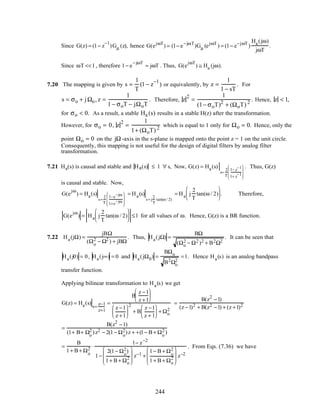
249. α =
1− B + Ωo
2
1+ B + Ωo
2 and β =
1− Ωo
2
1+ Ωo
2 . Now 1+ α =1+
1− B + Ωo
2
1+ B + Ωo
2 =
2(1+ Ωo
2 )
1+ B + Ωo
2 and
1− α =1−
1− B + Ωo
2
1+ B + Ωo
2 =
2B
1+ B + Ωo
2 . Hence, G(z) =
1− α
2
⋅
1− z−2
1−β(1+ α)z−1 + α z−2 which is the
same as that given in Eq. (4.113).
7.23 G(z) =
1 + α
2
⋅
1 − 2βz
−1
+ z
−2
1 −β(1 + α)z−1
+ αz−2
. For β = cosω0 the numerator of G(z) becomes
1 − 2cosω0z
−1
+ z
−2
= (1 − e
jω0
z
−1
)(1 − e
− jω0
z
−1
) which has roots at z = e
± jω0
. The
numerator of G(z
N
) is then given by (1 − e
jω0
z
−N
)(1 − e
− jω0
z
−N
) whose roots are obtained
by solving the equation z
N
= e
± jω0
, and are given by z = e
j(2πn±ω0)/N
, 0 ≤ n ≤ N −1.
Hence G(z
N
) has N complex conjugate zero pairs located on the unit circle at angles of
2πn ± ω0
N
radians, 0 ≤ n ≤ N −1.
ω0 = π / 2, there are 2N equally spaced zeros on the unit circle starting at ω = π / 2N.
7.24 (a) H(z) =
1
2
1 + A4 (z)[ ] =
N(z)
D(z)
where
A4(z) =
α1 −β1(1+ α1)z
−1
+ z
−2
1− β1(1+ α1)z−1
+α1z−2






α2 − β2(1 + α2)z
−1
+ z
−2
1− β2(1 + α2)z−1
+ α2 z−2





 . Therefore,
N(z) =
1
2
[ α1 −β1(1 + α1) z
−1
+ z
−2
( )α2 − β2(1 + α2)z
−1
+ z
−2
( )
+ 1 − β1(1 + α1)z
−1
+ α1 z
−2
( )1− β2(1 + α2)z
−1
+ α2 z
−2
( )]
=
1+ α1α2
2
{1 −
(1+ α1)(1 + α2)(β1 + β2)
1+ α1α2
z
−1
+
2[α1 + α2 + β1β2(1 + α1)(1 + α2)]
1 + α1α2
z
−2
−
(1 + α1)(1 + α2)(β1 + β2)
1+ α1α2
z
−3
+ z
−4
} which is seen to be a mirror-image
polynomial. We can express N(z) = a(1 + b1z
−1
+ b2z
−2
+ b1z
−3
+ z
−4
), where
(1): b1 = −
(1 + α1)(1 + α2)(β1 +β2 )
1 + α1α2
, (2): b2 =
2[α1 + α2 + β1β2(1 + α1)(1 + α2)]
1 + α1α2
, and
(b) (3): a =
1 + α1α2
2
.
(c) for z = e
jω
, we can write
N(e
jω
) = a(1 + b1e
−jω
+ b2e
− j2ω
+ b1e
− j3ω
+ e
− j4ω
) = ae
− j2ω
(b2 + 2b1cosω + 2cos2ω).
245

250. Now N(e
jωi
) = 0, for i = 1, 2. For i = 1 we get (4): b2 + 2b1cosω1 + 2 cos2ω1 = 0, and for
i = 2 we get (5): b2 + 2b1cosω2 + 2cos 2ω2 = 0. Solving Eqs. (4) and (5) we get
(6): b1 = −2(cosω1 + cosω2), and (7): b2 = 2(2cosω1 cosω2 +1).
From Eqs. (1) and (6) we have (8):
(1 + α1)(1 +α2)(β1 +β2 )
1 + α1α2
= 2(cosω1 + cosω2), and
from Eqs. (2) and (7) we have
(9):
2[α1 + α2 +β1β2(1 + α1)(1+ α2 )]
1+ α1α2
= 2(2cosω1 cosω2 +1). Substituting
α1 =
1 − tan(B1 / 2)
1 + tan(B1 / 2)
and α2 =
1 − tan(B2 / 2)
1 + tan(B2 / 2)
, and after rearrangement we get
(10): β1 +β2 = (cosω1 + cosω2) 1 + tan
B1
2




tan
B2
2









 =
∆
θ1, and
(11): β1β2 = 1+ tan
B1
2




tan
B2
2









 cosω1 cosω2 + tan
B1
2




tan
B2
2




=
∆
θ2.
The above two nonlinear equations can be solved resulting in
β1 =
θ1 ± θ1
2
− 4θ2
2
and β2 =
θ2
β1
.
(d) For the double notch filter with the following specifications: ω1 = 0.3π, ω2 = 0.5π,
B1 = 0.1π, and B2 = 0.15π, we get the following values for the parameters of the notch filter
transfer function: α1 = 0.7265, α2 = 0.6128, β1 = 0.5397, and β2 = 0.0705.
0 0.2 0.4 0.6 0.8 1
0
0.2
0.4
0.6
0.8
1
Ω
7.25 A zero (pole) of HLP(z) is given by the factor (z − zk ). After applying the lowpass-to-
lowpass transformation, this factor becomes
ˆz − α
1− α ˆz
− zk , and hence the new location of the
zero (pole) is given by the roots of the equation
246

251. ˆz − α − zk + α zk
ˆz = (1+ αzk )ˆz − (α + zk ) = 0 or ˆzk =
α + zk
1+ αzk
. For zk = −1,
ˆzk =
α −1
1− α
= −1.
7.26 The lowpass-to-bandpass transformation is given by z →
− b+ a ˆz − ˆz2
1− a ˆz + bˆz2 where a =
2αβ
β +1
and
b =
β −1
β +1
. A zero (pole) of HLP(z) is given by the factor (z − zk ). After applying the
lowpass-to-bandpass transformation, this factor becomes
− b + a ˆz − ˆz2
1− a ˆz + b ˆz2 − zk , and hence the new
location of the zero (pole) of the bandpass transfer function is given by the roots of the
equation (1+ bzk )z2
− a(1+ zk )z + (b+ zk ) = 0, or z2
−
a(1+ zk)
1+ bzk
z +
b + zk
1+ bzk
= 0, whose solution
is given by ˆzk =
a(1+ zk )
2(1+ bzk)
±
a(1+ zk )
2(1+ bzk)








2
−
b + zk
1+ bzk







 . For zk = −1, ˆzk = ±1.
7.27 For ωc = 0.42π and ˆω c = 0.57π we have α =
sin
ωc
− ˆω c
2






sin
ωc + ˆω c
2






=
sin(−0.075π)
sin(0.495π)
= −0.233474. Thus,
HLP(ˆz) = GLP (z)
z−1=
ˆz−1−α
1−αˆz−1
=
0.223 1+
ˆz−1
− α
1− α ˆz−1






2
1− 0.2952
ˆz−1 −α
1− α ˆz−1





 + 0.187
ˆz−1 − α
1− α ˆz−1






2
=
0.223(1− α)
2
(1+ ˆz
−1
)
2
(1+ 0.2952 α + 0.187α2
) +[−2α − 0.2952(1 + α2
) − 0.374α]ˆz−1
+(α2
+ 0.2952α + 0.187)ˆz−2
=
0.33929(1 + ˆz
−1
)
2
0.94127 + 0.24298 ˆz−1
+ 0.17259 ˆz−2
247

252. 0 0.2 0.4 0.6 0.8 1
-40
-30
-20
-10
0
ω/π
GLP
(z)
H
LP
(z)
7.28 For ωc = 0.42π and ˆω c = 0.61π we have α = −
cos
ωc
+ ˆω c
2






cos
ωc + ˆω c
2






= −
cos(0.515π)
cos(−0.95π)
= −0.0492852.
HHP(ˆz) = GLP (z)
z−1=−
ˆz−1 +α
1+αˆz−1
=
0.223 1−
ˆz−1
+ α
1+ α ˆz−1






2
1+ 0.2952
ˆz−1 + α
1+ α ˆz−1





 + 0.187
ˆz−1 + α
1+ α ˆz−1






2
=
0.223(1− α)2
(1− ˆz−1
)2
(1+ 0.2952α + 0.187α2) +[2α + 0.2952(1+ α2 )+ 0.374α]ˆz−1 +(α2 + 0.2952α + 0.187)ˆz−2
=
0.20156(1− ˆz−1
)2
1.015 + 0.41292 ˆz−1 + 0.20398ˆz−2 .
0 0.2 0.4 0.6 0.8 1
-40
-30
-20
-10
0
ω/π
HHP
(z) GLP
(z)
7.29 Since the passband edge frequencies are not specified, we assume the desired 3-dB bandwidth
of the bandpass filter HBP(z) is ˆω c2 − ˆω c1 = ωc,where ωc is the 3-dB cutoff frequency of
GLP(z) .
248

253. Moreover, the desired center frequency ˆω c is related to the passband edge frequencies through
ˆω c = ˆωc1
ˆω c2 or ˆω c
2
= ˆω c1
ˆωc 2. Hence,
( ˆω c2 + ˆω c1)
2
= ( ˆω c2 − ˆω c1)
2
+ 4 ˆω c2
ˆω c1 = ωc
2
+ 4 ˆω c
2
or ˆω c2 + ˆω c1 = ωc
2
+ 4 ˆω c
2
.
From Eq. (7.48) the lowpass-to-bandpass transformation is given by
z
−1
→ −z
−1 z
−1
− α
1 − αz−1
=
αz
−1
−z
−2
1− αz−1
, where α =
cos
ˆω c2 + ˆω c1
2






cos
ˆω c2 − ˆω c1
2






=
cos
ωc
2
+ 4 ˆω c
2
2








cos
ωc
2




.
For ωc = 0.42π and ˆω c = 0.45π, α = 0.013564 Then, HBP(z) = GLP(z)
z −1
→
δz
−1
−z
−2
1−δ z−1
=
0.223(1 − z
−2
)
2
1+ (−2α − 0.2952α)z−1
+ [α2
+ 0.2952(1 + α2
) + 0.187α2
]z−2
+(−0.2952α − 0.374α) z−3
+ 0.187z−4
=
0.1494(1 − z
−2
)
2
1− 0.036718z−1
+ 0.70738z−2
− 0.018832z−3
+ 0.3407z−4
.
0 0.2 0.4 0.6 0.8 1
-40
-30
-20
-10
0
ω/π
GLP
(z)
HBP
(z)
7.30 ωp = 0.6π, and ˆω p = 0.5π. Thus, α =
sin
ωp
− ˆω p
2








sin
ωp + ˆω p
2








=
sin 0.05π( )
sin(0.55π)
= 0.15838444.
Therefore, HHP(z) = GHP (z) z−1
→
z−1−α
1−αz−1
=
N(z)
D(z)
where
N(z) = 0.0916(1+ α)
3
(1 − z
−1
)
3
= 0.14238(1 − z
−1
)
3
and
D(z) = (1− 0.7601α + 0.7021α2
− 0.2088α3
)
+ [−3α + 0.7601(1+ 2α2
)− 0.7021(2α + α3
)+ 0.6264α2
]z−1
249

254. + [3α2
− 0.7601(2α + α3
)+ 0.7021(1+ 2α2
)− 0.6264α]z−2
+ (−α3
+ 0.7601α2
− 0.7021α+ 0.2088)z−3
= 0.896395 + 0.113602498z−1
+ 0.469574z−2
+ 0.1126927z−3
.
0 0.2 0.4 0.6 0.8 1
-25
-20
-15
-10
-5
0
5
ω /π
GHP
(z)HHP
(z)
7.31 HBP(z) =
0.136728736(1− z
−2
)
1 − 0.53353098z−1
+ 0.726542528z−2
. The lowpass-to-lowpass transformation is
given by z
−1
→
z
−1
− α
1 − αz−1
where α =
sin
ωo − ˆωo
2






sin
ωo + ˆω o
2






where ωo = 0.4π and ˆω o = 0.5π.
Thus, α = –0.15838.
GLP(z) = HLP(z) z
−1
=
z−1
−α
1−α z
−1
=
0.136728736 1 −
z−1
− α
1− α z
−1






2







1− 0.5335098
z−1
− α
1 − αz−1





 + 0.726542528
z−1
− α
1 − αz−1






2
=
0.136728736(1 − α)
2
(1 + ˆz
−1
)
2
(1+ 0.533531α + 0.72654253α2
) +[−2α − 0.533531(1 + α2
) −1.4531α]ˆz−1
+(α2
+ 0.533531 α + 0.72654253)ˆz−2
=
0.1333(1− ˆz
−2
)
0.93372 + 2.7299 ×10−9
× ˆz−1
+ 0.66713ˆz−2
.
250

255. 0 0.2 0.4 0.6 0.8 1
-25
-20
-15
-10
-5
0
5
ω /π
GBP
(z)HBP
(z)
7.32 The notch filter designed in Example 7.8 has notch frequency at ωo = 2π
60
400





 = 0.3π and its
transfer function is given by GBS(z) =
0.940809 −1.105987z
−1
+ 0.94089z
−2
1−1.105987z−1
+ 0.881618 z−2
. The desired
notch frequency of the transformed filter is ˆω o = 2π
100
400





 = 0.5π . The lowpass-to-lowpass
transformation to be used is given by z
−1
→
z
−1
− α
1 − αz−1
where α =
sin
ωo − ˆωo
2






sin
ωo + ˆω o
2






=
– 0.32492. The desired transfer function is thus given by
HBS(z) = GBS(z) z−1
=
z−1
−α
1−α z
−1
=
0.940809 −1.105987
z−1
− α
1− α z
−1





 + 0.94089
z−1
− α
1 − αz
−1






2
1−1.105987
z−1
− α
1 − αz−1





 + 0.881618
z−1
− α
1 − αz−1






2
=
(0.940809 +1.105987α + 0.940809 α2
) + [−3.7632α −1.105987(1 + α2
)]z−1
+(0.940809α2
+1.105987α + 0.940809)z−2
(1 +1.105987α + 0.940809α2
) + [−2 α −1.105987(1 + α2
) − 1.7632α]z−1
+(α2
+1.105987α + 0.881618)z−2
=
0.68078 + 3.4367 ×10
−7
z
−1
+ 0.68078z
−2
0.73997 + 3.4367 ×10−7
z−1
+ 0.62783z−2
.
251

256. 0 0.2 0.4 0.6 0.8 1
-25
-20
-15
-10
-5
0
5
ω /π
GBS
(z) HBS
(z)
7.33 GHP(z) =
0.0916(1− z−1
)3
1+ 0.7601z−1 + 0.7021z−2 + 0.2088z−3 . Now ωp = 0.6π, and ˆω p = 0.5π. Thus,
α = −
cos
ωp
+ ˆω p
2








cos
ωp − ˆω p
2








= −
cos(0.55π)
cos(0.05π)
= 0.15838444. Therefore,
HHP(z) = GHP(z) z
−1
→−
z−1
−α
1−α z
−1
=
N(z)
D(z)
, where N(z) = 0.0916(1+ α)3
(1+ z−1
)3
, and
D(z) = (1− 0.7601α + 0.7021α2
− 0.2088α3
)
+ [−3α + 0.7601(1+ 2α2
)− 0.7021(2α + α3
)+ 0.6264α2
]z−1
+ [3α2
− 0.7601(2α + α3
)+ 0.7021(1+ 2α2
)− 0.6264α]z−2
+ (−α3
+ 0.7601α2
− 0.7021α + 0.2088)z−3
0 0.2 0.4 0.6 0.8 1
-25
-20
-15
-10
-5
0
5
ω/π
GHP
(z)HLP
(z)
7.34 The ideal L-band digital filter HML(z) with an ideal frequency response given by HML(e
jω
)
= Ak for ωk−1 ≤ ω ≤ ωk , k = 1,2,K,L, can be considered as sum of L ideal bandpass filters
with cutoff frequencies at ωc1
k
= ωk −1 and ωc2
k
= ωk, where ωc1
0
= 0 and ωc2
L
= π. Now from
Eq. (7.90) the impulse response of a bandpass filter is given by hBP[n] =
sin(ωc2n)
πn
−
sin(ωc1n)
πn
. Therefore , hBP
k
[n]= Ak
sin(ωkn)
πn
−
sin(ωk−1n)
πn





. Hence,
252

257. hML[n] = hBP
k
[n]
k=1
L
∑ = Ak
sin(ωk n)
πn
−
sin(ωk−1n)
πn






k =1
L
∑
= A1
sin(ω1n)
πn
−
sin(0n)
πn





 + Ak
sin(ωkn)
πn
k =2
L −1
∑ − Ak
sin(ωkn)
πn
−
sin(ωk−1n)
πn






k=2
L −1
∑
+AL
sin(ωLn)
πn
−
sin(ωL−1n)
πn






= A1
sin(ω1n)
πn
+ Ak
sin(ωkn)
πn
− Ak
sin(ωk−1n)
πn
k=2
L−1
∑
k=2
L−1
∑ − AL
sin(ωL−1n)
πn
= Ak
sin(ωkn)
πn
− Ak
sin(ωk−1n)
πn
k=2
L
∑
k=1
L −1
∑ .
Since ωL = π, sin(ωLn) = 0. We add a term AL
sin(ωLn)
πn
to the first sum in the above
expression and change the index range of the second sum, resulting in
hML[n] = Ak
sin(ωkn)
πn
− Ak+1
sin(ωkn)
πn
k =1
L−1
∑
k=1
L
∑ .
Finally, since AL+1 = 0, we can add a term AL+1
sin(ωLn)
πn
to the second sum. This leads to
hML[n] = Ak
sin(ωkn)
πn
− Ak +1
sin(ωk n)
πn
= (Ak − Ak +1)
sin(ωkn)
πn
k=1
L
∑
k=1
L
∑
k=1
L
∑ .
7.35 HHT(e
jω
) =
j, −π < ω < 0,
−j, 0 < ω < π.



Therefore,
hHT[n]=
1
2π
HHT(e
jω
)e
jωn
dω
−π
0
∫ +
1
2π
HHT(e
jω
)e
jωn
dω
0
π
∫
=
1
2π
je
jωn
dω
−π
0
∫ −
1
2π
je
jωn
dω
0
π
∫ =
2
2πn
1− cos(πn)( ) =
2sin
2
(πn / 2)
πn
if n ≠ 0.
For n = 0, hHT[0] =
1
2π
jdω
−π
0
∫ −
1
2π
jdω
0
π
∫ = 0.
Hence, hHT[n]=
0, if n = 0,
2sin
2
(πn/ 2)
πn
, if n ≠ 0.




Since hHT[n]= − hHT[−n] and the length of the truncated impulse response is odd, it is a Type
3 linear-phase FIR filter.
253

258. From the frequency response plots given above, we observe the presence of ripples at the
bandedges due to the Gibbs phenomenon caused by the truncation of the impulse
response.
7.36 H x[n]{ }= hHT[n − k]x[k]
k =−∞
∞
∑ .
Hence F H x[n]{ }{ } = HHT(e
jω
)X(e
jω
) =
jX(ejω
), −π < ω < 0,
−jX(e
jω
), 0 < ω < π.




(a) Let y[n]= H H H H x[n]{ }{ }{ }{ }. Hence Y(e
jω
) =
j4
X(ejω
), −π < ω < 0,
(–j)
4
X(e
jω
), 0 < ω < π,




= X(e
jω
).
Therefore, y[n] = x[n].
(b) Define g[n]= H x[n]{ }, and h*[n]= x[n]. Then H x[l]{ }x[l ]
l =–∞
∞
∑ = g[l ]h*[l ]
l =–∞
∞
∑ .
But from the Parseval's' relation in Table 3.2, g[l ]h*[l ]
l =–∞
∞
∑ =
1
2π
G(e
jω
)
– π
π
∫ G(e
jω
)dω.
Therefore, H x[l]{ }x[l ]
l =–∞
∞
∑ =
1
2π
HHT(e
jω
)
−π
π
∫ X(e
jω
)X(e
– jω
)dω where
HHT(e
jω
) =
j, −π < ω < 0,
−j, 0 < ω < π.



Since the integrand HHT(e
jω
)X(e
jω
)X(e
– jω
) is an odd
function of ω , HHT(e
jω
)
−π
π
∫ X(e
jω
)X(e
– jω
)dω = 0. As a result, H x[l]{ }x[l ]
l =–∞
∞
∑ = 0.
7.37 HDIF(e
jω
)= jω. Hence,
hDIF[n] =
1
2π
jωe
jωn
−π
π
∫ dω=
j
2π
ω e
jωn
−π
π
∫ dω =
j
2π
ωe
jωn
jn
+
e
jωn
n
2







 −π
π
. Therefore,
hDIF[n] =
cos(πn)
n
−
sin(πn)
πn
2 =
cos(πn)
n
, if n ≠ 0. For n = 0, hDIF[0] =
1
2π
jω dω
−π
π
∫ = 0.
254

259. Hence, hDIF[n] =
0, n = 0,
cos(πn)
n
, | n| > 0.




Since hDIF[n] = – hDIF[–n], the truncated impulse
response is a Type 3 linear-phase FIR filter.
The magnitude responses of the above differentiator for several values of M are given below:
7.38 N = 2M + 1. ˆhHP[n] =
1−
ωc
π
, for n = M,
–
sin ωc(n− m)( )
π(n − m)
, if n ≠ M, 0 ≤ n < N,
0. otherwise.










Now ˆHHP(z) + ˆHLP (z) = ˆhHP[n]z
−n
n=−∞
∞
∑ + ˆhLP[n]z
−n
n=−∞
∞
∑ = ˆhHP[n]z
−n
n =0
N−1
∑ + ˆhLP[n]z
−n
n =0
N−1
∑
= ˆhHP [n]+ ˆhLP[n]( )z
−n
n =0
N −1
∑ .
But ˆhHP[n] + ˆhLP[n] = ˆhHP[n]+ ˆhLP[n]=
0, 0≤ n ≤ N –1, n ≠ M,
1, n = M,



,
Hence, ˆHHP(z) + ˆHLP (z) = z
–M
,i.e. the two filters are delay-complementary.
255

260. 7.39 HLLP(e
jω
) =
ω, ω < ωc
,
0, otherwise.



Therefore,
hLLP[n]=
1
2π
− ωejωn
dω
−ωc
0
∫ + ωejωn
dω
0
ωc
∫










=
1
2π
−
ωejωn
jn
+
ejωn
n2








–ωc
0
+
ω ejωn
jn
+
ejωn
n2








0
ωc










=
1
2π
ωce
jωc
n
−ωce
−jωc
n
jn
+
e
jωc
n
+ e
−jωc
n
− 2
n
2







 =
ωc
πn
sin(ωcn) +
cos(ωcn)−1
π n
2 .
7.40 HBLDIF(e
jω
) =
ω, ω < ωc
,
0, otherwise.



Hence,
hBLDIF[n]=
1
2π
ωe
jωn
dω
−ωc
ωc
∫ =
1
2π
ωe
jωn
jn
+
e
jωn
n
2








−ωc
ωc










=
1
2π
ωcejωcn + ωce−jωcn
jn
+
e jωc
n
− e−jωc
n
n2








= – j
ωc
πn
cos(ωcn) + j
1
πn2 sin(ωcn).
7.41 From Eq. (2.181) y(nT) = y (n−1)T( )+ x(τ)dτ
(n −1)T
nT
∫ = y (n− 1)T( )+ T ⋅x (n− 1)T( ) which reduces to
y[n] = y[n −1]+ T⋅x[n −1]. Hence, the corresponding transfer function is given by
HR(z) =
Tz−1
1− z−1 . From Eq. (2.99) y[n] = y[n −1]+
T
2
x[n]+ x[n− 1]( ). Hence, the corresponding
transfer function is given by HT(z) =
T
2
⋅
1+ z−1
1− z−1 . From the plot given below it can be seen that
the magnitude response of Hint(z) lies between that of HR(z) and HT(z).
0.2 0.4 0.6 0.8 1
0
0.5
1
1.5
ω/π
H
int
(z)
HR(z)
H
T
(z)
7.42 HN(z) =
3
4
HR(z) +
1
4
HR(z) . From the plot given below it can be seen that the magnitude
response of HN(z) lies between that of HR(z) and HT(z), and is much closer to that of
Hint(z) .
256

261. 0.2 0.4 0.6 0.8 1
0
0.5
1
1.5
ω/π
H
int
(z)
HR
(z)
H
T
(z)
H
N
(z)
7.43 HN(z) =
3
4
z
−1
1− z−1





 +
1
8
1+ z
−1
1− z−1





 =
1+ 7 z
−1
8(1 − z−1
)
. Its inverse is given by H(z) =
8(1 − z
−1
)
1+ 7z−1
,
which is unstable as it has a pole at z = –7. A stable transfer function with the same magnitude
response is obtained by multiplying H(z) with an allpass function (1 + 7z
−1
) / (7 +z
−1
)
resulting in HIIR(z) =
8(1 − z
−1
)
1+ 7z−1
⋅
1+ 7z
−1
7 + z−1
=
8(1− z
−1
)
7 +z−1
, A plot of the ideal differentiator
Hdif (z) with a frequency response given by Eq. (7.68) and that of the IIR differentiator
HIIR(z) is given below. As can be seen the magnitude response of HIIR(z) is very close to
that Hdif (z) .
0 0.2 0.4 0.6 0.8 1
0
0.5
1
1.5
2
2.5
3
ω /π
Hdif
(z)
HIIR
(z)
7.44 The frequency response of a causal ideal notch filter can thus be expressed as
Hnotch(e
jω
) =
(
Hnotch(ω)e
jθ(ω)
where
(
Hnotch(ω) is the amplitude response which can be
expressed as
(
Hnotch(ω) =
1, 0 ≤ ω < ωo
−1, ωo ≤ ω < π.



It follows then that
(
Hnotch(ω) is related to the
amplitude response
(
HLP(ω) of the ideal lowpass filter with a cutoff at ωo through
(
Hnotch(ω) = ±2
(
HLP(ω) −1[ ]. Hence, the impulse response of the ideal notch filter is given
by hnotch[n] = ±2 hLP[n]) − δ[n][ ], where hLP[n] =
sin(ωon)
πn
, −∞ < n < ∞. The
257

262. magnitude responses of a length 41 notch filter with a notch frequency at ωo = 0.4π and its
associated length-41 lowpass filter are shown below.
0 0.2 0.4 0.6 0.8 1
0
0.5
1
1.5
ω /π
ωo
= 0.4π
7.45 (a) See Section 10.5.2
(b) D = 100/11. h[n] =
D − k
n − k



k=0
k≠n
16
∏ , 0 ≤ n ≤ 16.
h[0] = –8.8187e-07, h[1] = 1.5854e-05, h[2] = –1.3567e-04,
h[3] = 7.3708e-04, h[4] = –2.8661e-03, h[5] = 8.5600e-03,
h[6] = –2.0771e-02, h[7] = 4.3863e-02, h[8] = –4580e-02, h[9] = 1.0089e+00,
h[10] = 7.0620e-02, h[11] = –1.8343e-02, h[12] = 5.0156e-03,
h[13] = –1.1485e-03, h[14] = 1.9597e-04, h[15] = –2.1708e-05, h[16] = 1.1604e-06.
0 0.2 0.4 0.6 0.8 1
8
8.5
9
9.5
10
ω /π
Ideal
Lagrange
7.46 Note that the desired delay D = 9.0909. Hence N = 9 is the order of the allpass transfer
function. The allpass fractional delay are thus given by A(z) =
z−9
D(z−1
)
D(z)
where
D(z) = 1− 0.81081z−1
+ 0.031901z−2
− 0.012872z−3
+ 0.0045589z−4
− 0.0013236z−5
+ 2.9767 ×10−4
z−6
− 4.829 × 10−5
z−7
− 5.0088 × 10−6
z−8
+ 2.489× 10−7
z−9
.
258

263. 0 0.2 0.4 0.6 0.8 1
8
8.5
9
9.5
10
ω/π
Ideal
Allpass
7.47 (a) x[n] = s[n] + Ak
k= 0
M
∑ sin(kωon + φk ) = s[n] + r[n], where s[n] is the desired signal and
r[n] = Ak
k=0
M
∑ sin(k ωon + φk ) is the harmonic interference with fundamental frequency ωo .
Now, r[n − D] = Ak
k=0
M
∑ sin kωo(n − D) + φk[ ]) = Ak
k=0
M
∑ sin(k ωon + φk − 2πk) = r[n].
(b) y[n] = x[n] − x[n − D] = s[n]+ r[n]− s[n − D] − r[n − D] = s[n] + r[n] − s[n − D] − r[n]
= s[n] − s[n − D]. Hence, y[n] does not contain any harmonic disturbances.
(c) Hc (z) =
1 − z
−D
1 − ρD
z−D
. Thus,
Hc (e
jω
) =
1 − e
− jDω
1 − ρD
e− jDω
=
1 − cos(Dω)( )+ jsin(Dω)
1− ρD
cos(Dω)( )+ jρD
sin(Dω)
. Then
Hc (e
jω
) =
2 1 − cos(Dω)( )
1 − 2ρD
cos(Dω) + ρ2D
. A plot of Hc (e
jω
) for ωo = 0.22π and ρ = 0.99 is
shown below:
-1 -0.5 0 0.5 1
0
0.5
1
1.5
ω /π
(d)
259

264. x[n] y[n]
+–
z–D
7.48 Hc (z) =
P(z)
Q(z)
=
1 − N(z)
1 − (0.985)(100/11)
N(z)
where the coefficients of N(z) are as given in
Problem 7.45 solution. The transfer function coefficients in ascending powers of z
−1
are
given by
Numerator Coefficients
Columns 1 through 5
1.0000e+00 -1.5854e-05 1.3567e-04 -7.3708e-04 2.8661e-03
Columns 6 through 10
-8.5600e-03 2.0771e-02 -4.3863e-02 9.4580e-02 -1.0089e+00
Columns 11 through 15
-7.0620e-02 1.8343e-02 -5.0156e-03 1.1485e-03 -1.9597e-04
Columns 16 through 17
2.1708e-05 -1.1604e-06
Denominator Coefficients
Columns 1 through 5
1.0000e+00 -1.3819e-05 1.1826e-04 -6.4246e-04 2.4981e-03
Columns 6 through 10
-7.4611e-03 1.8104e-02 -3.8232e-02 8.2439e-02 -8.7934e-01
Columns 11 through 15
-6.1554e-02 1.5988e-02 -4.3717e-03 1.0010e-03 -1.7081e-04
Columns 16 through 17
1.8921e-05 -1.0114e-06
-1 -0.5 0 0.5 1
0
0.5
1
1.5
ω/π
ρ = 0.985
260

265. 7.49 Hc (z) =
P(z)
Q(z)
=
D(z) − z
−9
D(z
−1
)
D(z) − (0.99)(100/11)
z−9
D(z−1
)
where
P(z) = 1− 0.81086 z
−1
+ 0.031949z
−2
− 0.01317z
−3
+ 0.0058825z
−4
− 0.0058825z
−5
+ 0.01317z
−6
− 0.031949z
−7
+ 0.0810869z
−8
−z
−9
, and
Q(z) = 1 − 0.81086z
−1
+ 0.031945z
−2
− 0.013144z
−3
+ 0.0057669z
−4
− 0.0054844z
−5
+ 0.012046z
−6
− 0.029164z
−7
+ 0.074006 z
−8
−0.91268z
−9
,
-1 -0.5 0 0.5 1
0
0.5
1
1.5
ω/π
ρ = 0.99
7.50 HLP(e
jω
) =
1, −ωp
≤ ω ≤ ωp
,
1−
ω − ωp
ωs − ωp








, ωp
< ω ≤ ωs
,
1+
ω + ωp
ωs
− ωp







 , − ωs < ω ≤ ωp,
0, elsewhere.












Now, for n ≠ 0, hLP[n] =
1
2π
HLP(e
jω
)e
jωn
dω
−π
π
∫
=
1
2π
e
jωn
dω
−ωp
ω p
∫ + 1−
ω − ωp
∆ω







 e
jωn
dω + 1+
ω + ωp
∆ω







 e
jωn
dω
−ωs
−ωp
∫
ωp
ωs
∫












=
1
2π
e
jωn
dω
−ωs
ωs
∫ −
ω − ωp
∆ω
e
jωn
dω +
ω + ωp
∆ω
e
jωn
dω
−ωs
−ωp
∫
ωp
ωs
∫












=
1
2π
2sin(ωsn)
πn
−
1
∆ω
(ω − ωp )ejωn
jn
+
ejωn
n2









 ωp
ωs
+
1
∆ω
(ω +ωp )ejωn
jn
+
ejωn
n2









 – ωs
– ωp












=
1
2π
2sin(ωsn)
πn
−
1
∆ω
∆ωejωs
n
jn
+
ejωs
n
− ejωp
n
n2 +
−∆ωe−jωs
n
jn
−
e−jω p
n
− e−jωs
n
n2
















261

266. =
1
2π
2sin(ωsn)
πn
−
2
∆ω
∆ωsin(ωsn)
n
+
cos(ωsn)− cos(ωpn)
n2
















=
1
∆ω
cos(ωpn)
πn
2 −
cos(ωsn)
πn
2








=
1
∆ω
cos((ωc − ∆ω / 2)n)
πn
2 −
cos((ωc + ∆ω / 2)n)
πn
2






=
2sin(∆ωn/ 2)
∆ωn
sin(ωcn)
πn
.
Now for n = 0, hLP[0] =
1
2π
HLP (e
jω
)dω
−π
π
∫ =
1
2π
(area under the curve)
=
1
2π
2 ωs + ωp( )
2
=
ωc
π
.
Hence, hLP[n] =
ωc
π
, if n = 0,
2sin(∆ωn / 2)
∆ωn
sin(ωcn)
πn
, if n ≠ 0.






An alternate approach to solving this problem is as follows. Consider the frequency
response G(ejω
) =
dHLP (ejω )
dω
=
0, −ωp
≤ ω ≤ ωp
,
–
1
∆ω
, ωp
< ω < ωs
,
1
∆ω
, −ωs < ω < −ωp,
0, elsewhere.









Its inverse DTFT is given by
g[n]=
1
2π
G(ejω
)ejωn
dω
–π
π
∫ =
1
2π
1
∆ω
–ωs
–ωp
∫ ejωn
dω −
1
2π
1
∆ω
ωp
ωs
∫ ejωn
dω
=
1
2π∆ω
−ωs
−ωp
ejωn
jn
−
ωp
ωs
ejωn
jn










=
1
jπn∆ω
cos(ωpn) − cos(ωsn)( ).
Thus, hLP[n] =
j
n
g[n] =
1
πn2 ∆ω
cos(ωpn)− cos(ωsn)( )
=
1
πn2 ∆ω
cos ωc −
∆ω
2





 n





 − cos ωs +
∆ω
2





 n














=
2sin(∆ωn/ 2)
∆ωn
⋅
sin(ωcn)
πn
, for n ≠ 0.
For n = 0, hLP[n] =
ωc
π
.
7.51 Consider the case when the transition region is approximated by a second order spline. In
this case the ideal frequency response can be constructed by convolving an ideal, no-
262

267. transition-band frequency response with a triangular pulse of width ∆ω = ωs − ωp , which in
turn can be obtained by convolving two rectangular pulses of width ∆ω / 2. In the time
domain this implies that the impulse response of a filter with transition band approximated by
a second order spline is given by the product of the impulse response of an ideal low pass
filter with no transition region and square of the impulse response of a rectangular pulse.
Now,
HLP(ideal)[n] =
sin(ωcn)
πn
and Hrec[n] =
sin(∆ωn/ 4)
∆ωn/ 4
. Hence, HLP[n]= HLP(ideal)[n] Hrec[n]( )2
.
Thus for a lowpass filter with a transition region approximated by a second order spline
hLP[n] =
ωc
π
, if n = 0,
sin(∆ωn/ 4)
∆ωn / 4






2 sin(ωc
n)
πn
, otherwise.







Similarly the frequency response of a lowpass filter with the transition region specified by a
P-th order spline can be obtained by convolving in the frequency domain an ideal filter with
no transition region with P rectangular pulses of width ∆ω /P. Hence,
HLP[n]= HLP(ideal)[n] Hrec[n]( )P
, where the rectangular pulse is of width ∆ω /P. Thus
hLP[n] =
ωc
π
, if n = 0,
sin(∆ωn/ 2P)
∆ωn / 2P






P sin(ωc
n)
πn
, otherwise.







7.52 Consider another filter with a frequency response G(e
jω
) given by
G(e
jω
) =
0, 0 ≤ ω ≤ ωp
,
−π
2∆ω
sin
π(ω − ωp
)
∆ω







, ωp < ω ≤ ωs,
−π
2∆ω
sin
π(ω + ωp)
∆ω







, −ωs
≤ ω ≤ −ωp
,
0, elsewhere.











Clearly G(e
jω
) =
dH(e
jω
)
dω
. Now,
g[n] =
1
2π
G(e
jω
)e
jωn
dω
−π
π
∫ =
−π
8π∆ωj
e
j
π(ω−ωp)
∆ω






e
jωn
dω
ωp
ωs
∫ − e
−j
π(ω−ω p)
∆ω






e
jωn
dω
ωp
ωs
∫






+ e
j
π(ω+ωp )
∆ω






e
jωn
dω
−ωs
−ωp
∫ − e
−j
π(ω+ωp )
∆ω






e
jωn
dω
−ωs
−ωp
∫





263

268. =
−1
8∆ωj
e
(−jπωp
/ ∆ω) e
jωs
(n+π / ∆ω)
− e
jω p
(n+π/ ∆ω)
j(n + π / ∆ω)










− e
(jπωp
/ ∆ω) e
jωs
(n −π / ∆ω)
− e
jωp
(n−π / ∆ω)
j(n− π / ∆ω)















+e
(jπωp
/ ∆ω) e
−jω p
(n+π/ ∆ω)
− e
−jωs
(n+π/ ∆ω)
j(n + π / ∆ω)










− e
(−jπωp
/ ∆ω) e
−jωp
(n −π/ ∆ω)
− e
−jωs
(n −π / ∆ω)
j(n − π / ∆ω)















=
−1
4∆ωj
−sin(ωs n) − sin(ωp n)
(n + π / ∆ω)
−
−sin(ωsn)− sin(ωpn)
(n − π / ∆ω)







 =
sin(ωsn)+ sin(ωpn)( )
4∆ωj
−2π / ∆ω
n
2
− π
2
/ ∆ω
2








=
sin(ωcn)cos(∆ωn / 2)
∆ωj
1
π 1−(∆ω / π)
2
n
2

















.
Now h[n] =
j
n
g[n]. Therefore, h[n] =
cos(∆ωn / 2)
1− (∆ω/ π)
2
n
2






sin(ωcn)
πn





.
7.53 Let wR[n] =
1
k
, Since the convolution of two length N sequences produces a sequence of
length 2N– 1, therefore 2N –1 = 2M + 1 which gives N = M + 1. Therefore, wR[n] =
1
k
,
–
M
2
≤ n ≤
M
2
. Now, w[n] = wR[n] * wR[n] =
1
k2
M +1− n( ), −M ≤ n ≤ M,
0, elsewhere,




or
w[n] =
M +1
k
2 1−
n
M +1





 , −M ≤ n ≤ M,
0, elsewhere.





,
Now
M +1
k
2 =1 which yields k = M +1 . Hence a Bartlett window of length 2M + 1 is
obtained by the linear convolution of 2 length M + 1 rectangular windows scaled by a factor
of
1
M + 1
each. The DTFT ΨBART(e
jω
) of the Bartlett window is thus given by
ΨBART(e
jω
) = ΨR(e
jω
)( )
2
=
1
M +1
sin2 ω(M+1)
2( )
sin
2 ω
2( )
, where ΨR(e
jω
) is the DTFT of the
rectangular window. Hence ΨBART(e
jω
) = 0 at ω = ±
2π
M +1
, ±
4π
M +1
, ......
Therefore ∆ML,BART =
4π
M +1
. It should be noted that the main lobe width given here is for a
Bartlett window of length 2M + 1 = 2N – 1 as compared to that of a rectangular window of
length N = M + 1. The maximas of the DTFT ΨBART(e
jω
) of the Bartlett window occur at the
same location as the DTFT ΨR(e
jω
) of the rectangular window. Since ΨBART(e
jω
) =
ΨR(e
jω
)( )
2
, it follows then Asl ,BART = 2× Asl ,R = 2 ×13.3= 26.6 dB.
264

269. 7.54 wGC[n] = α + βcos
2πn
2M + 1





 + γ cos
4πn
2M +1











wR[n]
= α + 2β e
j
2πn
2M+1




+ e
−j
2πn
2M+1














+ 2γ e
j
4πn
2M+1




+ e
−j
4πn
2M+1
























wR[n]
Hence, ΨGC (e
jω
) = α ΨR(e
jω
) + 2β ΨR e
j ω−
2π
2M+1














+ 2βΨR e
j ω+
2π
2M+1














+ 2γ ΨR e
j ω−
4π
2M+1














+ 2γ ΨR e
j ω+
4π
2M+1














.
For the Hann window : α = 0.5, β = 0.5 and γ = 0. Hence
ΨHANN(e
jω
) = 0.5ΨR(e
jω
) + ΨR e
j ω−
2π
2M+1














+ ΨR e
j ω+
2π
2M+1














= 0.5
sin
(2M +1)ω
2






sin(ω/ 2)
+
sin (2M +1)
ω
2
−
π
2M +1












sin
ω
2
−
π
2M +1






+
sin (2M +1)
ω
2
+
π
2M +1












sin
ω
2
+
π
2M +1






.
For the Hamming window α = 0.54, β = 0.46, and γ = 0. Hence
ΨHAMMING(e
jω
) = 0.54 ΨR(e
jω
) + 0.92 ΨR e
j ω−
2π
2M+1














+0.92ΨR e
j ω+
2π
2M+1














.
= 0.54
sin
(2M +1)ω
2






sin(ω/ 2)
+ 0.92
sin (2M +1)
ω
2
−
π
2M +1












sin
ω
2
−
π
2M +1






+ 0.92
sin (2M + 1)
ω
2
+
π
2M + 1












sin
ω
2
+
π
2M +1






..
For the Blackmann window α = 0.42, β = 0.5 and γ = 0.08
ΨBLACK (e
jω
) = 0.54ΨR(e
jω
) +ΨR e
j ω−
2π
2M+1














+ WR e
j ω+
2π
2M+1














+ 0.16 ΨR e
j ω−
4π
2M+1














+ 0.16 ΨR e
j ω−
4π
2M+1














= 0.42
sin
(2M +1)ω
2






sin(ω/ 2)
+
sin (2M +1)
ω
2
−
π
2M +1












sin
ω
2
−
π
2M +1






+
sin (2M +1)
ω
2
+
π
2M +1












sin
ω
2
+
π
2M +1






265

270. + 0.16
sin (2M +1)
ω
2
−
2π
2M +1












sin
ω
2
−
2π
2M + 1






+ 0.16
sin (2M +1)
ω
2
−
2π
2M +1












sin
ω
2
−
2π
2M +1






.
7.55 (a) N = 1 and hence, xa(t) = α0 + α1t. Without any loss of generality, for L = 5, we first
fit the data set {x[k]}, −5 ≤ k ≤ 5, by the polynomial xa(t) = α0 + α1t with a minimum mean-
square error at t = –5, –4, . . . , 0, 1, . . , 5, and then replace x[0] with a new value x[0] =
xa(0) = α0 .
Now, the mean-square error is given by e(α0,α1) = x[k]− α0 – α1k{ }2
k=−5
5
∑ . We set
∂ε(α0,α1)
∂α0
= 0 and
∂ε(α0,α1)
∂α1
= 0 which yields 11α0 + α1 k
k=−5
5
∑ = x[k],
k=−5
5
∑ and
α0 k
k=−5
5
∑ + α1 k2
k =−5
5
∑ = k x[k].
k =−5
5
∑
From the first equation we get x[0] = α0 =
1
11
x[k]
k =−5
5
∑ . In the general case we thus have
x[n] = α0 =
1
11
x[n − k]
k=−5
5
∑ , which is a moving average filter of length 11.
(b) N = 2 and hence, xa(t) = α0 + α1t + α2t2
. Here, we fit the data set {x[k]}, −5 ≤ k ≤ 5, by
the polynomial xa(t) = α0 + α1t + α2t2
with a minimum mean-square error at t = –5, –4, . . . ,
0, 1, . . , 5, and then replace x[0] with a new value x[0] = xa(0) = α0 . The mean-square
error is now given by ε α0,α1,α2( )= x[k]− α0 −α1k − α2k2
( )
2
k =−5
5
∑ . We set
∂ε(α0,α1,α2)
∂α0
= 0,
∂ε(α0,α1,α2)
∂α1
= 0, and
∂ε(α0,α1,α2)
∂α2
= 0, which yields
11α0 +110α2 = x[k],
k=−5
5
∑ 110α1 = kx[k],
k =−5
5
∑ 110α0 + 1958α2 = k2
x[k].
k =−5
5
∑ From the first
and the third equations we then get
α0 =
1958 x[k]
k=−5
5
∑ −110 k2
x[k]
k =−5
5
∑
(1958 ×11) −(110)2 =
1
429
89 − 5k2
( )
k =−5
5
∑ x[k].
Hence, here we replace x[n] with a new value x[n] = α0 which is a weighted combination of
the original data set {x[k]}, −5 ≤ k ≤ 5:
x[n] =
1
429
89 − 5k2
( )
k=−5
5
∑ x[n − k]
=
1
429
(−36 x[n+ 5]+ 9x[n + 4]+ 44 x[n + 3]+ 69x[n + 2] +84 x[n +1]+ 89 x[n]
266

271. + 84x[n −1]+ 69x[n − 2]+ 44x[n − 3]+ 9x[n − 4]− 36x[n − 5]).
(c) The impulse response of the FIR filter of Part (a) is given by
h1[n]=
1
11
1 1 1 1 1 1 1 1 1 1 1{ },
whereas, the impulse response of the FIR filter of Part (b) is given by
h1[n]=
1
429
−36 9 44 69 84 89 84 69 44 9 −36{ }.
The corresponding frequency responses are given by
H1(ejω
) =
1
11
e−jωk
k =−5
5
∑ , and H2(ejω
) =
1
429
89− 5k2
( )e−jωk
k=−5
5
∑ .
A plot of the magnitude responses of these two filters are shown below from which it can be
seen that the filter of Part (b) has a wider passband and thus provides smoothing over a larger
frequency range than the filter of Part (a).
7.56 y[n] =
1
320
{– 3x[n – 7] – 6x[n – 6] – 5x[n – 5] + 3x[n – 4] + 21x[n – 3] + 46x[n – 2]
+ 67x[n – 1] + 74x[n] + 67x[n + 1] + 46x[n + 2] + 21x[n + 3]
+ 3x[n + 4]5x[n + 5] – 6x[n + 6] – 3x[n + 7] }.
Hence,
Y(e
jω
)
X(e
jω
)
=
1
320
−3e
−j7ω
− 6e
−j6ω
− 5e
−j5ω
+ 3e
−j4ω
+ 21e
−j3ω
+ 46 e
−j2ω
+ 67e
−jω
+ 74{
+ 67e
jω
+ 46e
j2ω
+ 21e
j3ω
+ 3e
j4ω
− 5e
j5ω
− 6e
j6ω
− 3e
j7ω
}.
Thus, H(e
jω
) =
Y(e
jω
)
X(e
jω
)
=
1
160
74{ + 67cosω + 46cos(2ω) + 21cos(3ω) + 3cos(4ω)
–5cos(5ω) –6cos(6ω) –3cos(7ω)}.
The magnitude response of the above FIR filter is plotted below (solid line marked 's') along
with that of the FIR filter of Part (b) of Problem 7.25 (dashed line marked '(b)'). Note that
both filters have roughly the same passband but the Spencer's filter has very large attenuation
in the stopband and hence it provides better smoothing than the filter of Part (b).
267

272. 7.57 (a) L = 3. P(x) = α1x+ α2x
2
+ α3x
3
. Now P(0) = 0 is satisfied by the way P(x) has been
defined. Also to ensure P(1) = 1 we require α1 + α2 + α3 = 1. Choose m = 1 and n = 1,
Since
dP(x)
dx x=0
= 0, hence α1 + 2α2x + 3α3x
2
x=0
= 0, implying α1 = 0. Also since
dP(x)
dx x=1
= 0 , hence α1 + 2α2 + 3α3 = 0 . Thus solving the three equations:
α1 + α2 + α3 = 1, α1 = 0, and α1 + 2α2 + 3α3 = 0
we arrive at α1 = 0, α2 = 3, and α3 = –2. Therefore, P(x) = 3x
2
–2x
3
.
(b) L = 4. Hence, P(x) = α1x+ α2x
2
+ α3x
3
+ α4x
4
. Choose m = 2 and n = 1 (alternatively
one can choose m = 1 and n = 2 for better stopband performance ). Then,
P(1) = 1 ⇒ α1 + α2 + α3 + α4 =1,
dP(x)
dx x=0
= 0 ⇒ α1 + 2α2x + 3α3x
2
+ 4α4x
3
x=0
= 0,
d
2
P(x)
dx
2 x=0
= 0 ⇒ 2α2 + 6α3x +12α4x
2
x =0
= 0,
dP(x)
dx x=1
= 0 ⇒ α1 + 2α2 + 3α3 + 4α4 = 0 .
Solving the above simultaneous equations we get α1 = 0, α2 = 0, α3 = 4, and α4 = –3.
Therefore, P(x) = 4x
3
− 3x
4
.
(c) L = 5. Hence P(x) = α1x+ α2x
2
+ α3x
3
+ α4x
4
+ α5x
5
. Choose m = 2 and n = 2.
Following a procedure similar to that in parts (a) and (b) we get α1 = 0, α2 = 0, α3 = 10,
α4 = –15, and α5 = 6.
268

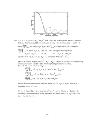
273. 7.58 From Eq. (7.102) we have
(
H(ω) = c[k]sin(
k=1
M
∑ ωk). Now
(
H(π − ω) = c[k]sin (ω − π)k( )
k=1
M
∑ = − c[k]sin(
k=1
M
∑ ωk) cos(πk) = c[k](−1)
k+1
sin(
k=1
M
∑ ωk).
Thus,
(
H(ω) =
(
H(π − ω) implies c[k]sin(
k=1
M
∑ ωk) = c[k](−1)
k+1
sin(
k=1
M
∑ ωk), or equivalently,
1 − (−1)
k+1
( )c[k]sin(
k=1
M
∑ ωk) = 0 which in turn implies that c[k] = 0 for k = 2, 4, 6, .... .
But from Eq. (7.103) we have c[k] = 2 h[M − k], 1 ≤ k ≤ M. Or, h[k] =
1
2
c[M − k]. For k
even, i.e., k = 2R, h[2R] =
1
2
c[M − 2R] = 0 if M is even.
7.59 (a) H[k] = H(e
jωk
) = H(e
j2πk /M
), 0 ≤ k ≤ M −1. Thus, h[n] =
1
M
H[k]WM
− kn
k=0
M−1
∑ ,
where WM = e
− j@π/M
.
Now, H(z) = h[n]z
− n
n= 0
M−1
∑ =
1
M
H[k]
k=0
M−1
∑
n=0
M−1
∑ WM
− kn
z
−n
=
1
M
H[k] WM
− kn
z
−n
n=0
M−1
∑






k=0
M−1
∑ .
We can write WM
− kn
z
−n
n=0
M−1
∑ = WM
− kn
z
−n
n=0
∞
∑ − WM
− kn
z
−n
n=M
∞
∑
= WM
− kn
z
− n
n=0
∞
∑ − WM
−kM
z
−M
WM
− kn
z
− n
n=0
∞
∑ = 1 − z
−M
( ) WM
− kn
z
−n
n= 0
∞
∑ =
1− z
−M
1 − WM
− k
z−1
.
Therefore, H(z) =
1 − z
−M
M
H[k]
1 − WM
−k
z−1
k=0
M−1
∑ .
(b)
269

274. H[0]
M
H[1]
M
H[M− 1]
M
x[n] y[n]
1
1− z−1
1
1− z−1e j2π/ M
1
1− z−1e j2π(M−1)/ M
1− z−M
(c) On the unit circle
7.60 (a) For Type 1 FIR filter, H(e
jω
) = e−j
ω(M−1)
2 H(e
jω
) . Since in frequency sampling
approach we sample the DTFT H(e
jω
) at M points given by ω =
2πk
M
, k = 0,1,K,M −1,
therefore H[k]= H(ej2πk / M
) = Hd (ej2πk / M
) e−j2πk(M−1)/ 2M
, k = 0,1,K,M −1. Since the
filter is of Type 1, (M – 1) is even, thus ej2π(M−1) /2
=1. Moreover, h[n] being real,
H(ejω
) = H*(ejω
). Thus, H(ejω
) = ejω(M−1)/ 2
H(ejω
),, π ≤ ω < 2π. Hence,
H[k]=
Hd(ej2πk / M
) e−j2πk(M−1)/ 2M
, k = 0,1,2,K,
M−1
2
,
Hd(ej2πk / M
) ej2π(M−k)(M−1)/ 2M
, k =
M+1
2
,
M+3
2
,K,M −1.





(b) For Type 2 FIR filter
H[k]=
Hd
(ej2πk / M) e−j2πk(M−1)/ 2M, k = 0,1,2,K,
M
2
−1,
0, k =
M
2
,
Hd(ej2πk / M
) ej2πk(M−k)(M−1) /2M
k =
M
2
+ 1,K,M −1.







7.61 (a) The frequency spacing between two consecutive samples is given by
2π
17
= 0.11765π, and
hence the desired passband edge ωp = 0.5π is between the frequency samples at
ω =
2π × 4
17
= 0.47059π and ω =
2π × 5
17
= 0.58824π. From Eq. (7.174) the specified DFT
samples are thus given by
H[k] =
e−j(2π /17)8
, k = 0,1,K,4,12,K,16,
0, k = 5,K,11.




(b) A 17-point inverse DFT of the above DFT samples yields the impulse response coefficients
given below in ascending powers of z
−1
:
Columns 1 through 5
270

275. 4.3498e-03 6.0460e-03 -2.9166e-02 8.1624e-03 5.7762e-02
Columns 6 through 10
-6.4003e-02 -7.9934e-02 3.0267e-01 5.8824e-01 3.0267e-01
Columns 11 through 15
-7.9934e-02 -6.4003e-02 5.7762e-02 8.1624e-03 -2.9166e-02
Columns 16 through 17
6.0460e-03 4.3498e-03
0 0.2 0.4 0.6 0.8 1
0
0.5
1
1.5
ω/π
0 0.2 0.4 0.6 0.8 1
-60
-50
-40
-30
-20
-10
0
ω /π
7.62 (a) ωp = 0.3π. For M = 37, the frequency spacing between two consecutive frequency
samples is
2π
37
= 0.054054π. Hence, the desired passband edge of the lowpass filter is between
the frequency sample at ω =
2π × 5
37
= 0.27027π and ω =
2π × 6
37
= 0.3243243π . N = 37, and
Hd (e
jω
) =
1, 0< ω ≤ 0.3π,
0, 0.3π < ω ≤ 1.7π,
1, 1.7π < ω ≤ 2π.





Therefore, H[k]=
e−j(2πk / 37)18, 0 ≤ k < 6,
0, 6 ≤ k < 32,
ej(2π(37−k)/ 37)18, 32 ≤ k ≤ 36.






Hence, H[k]=
e−j(2πk / 37)18
, k = 0,1,K,5,32,33,K,36,
0, k = 6,7,K,31.




(b) A 37-point inverse DFT of the above DFT samples yields the impulse response coefficients
given below in ascending powers of z
−1
:
Columns 1 through 5
-2.4155e-02 -4.6049e-03 1.9130e-02 2.8037e-02 1.4205e-02
Columns 6 through 10
-1.2467e-02 -3.1027e-02 -2.5234e-02 3.0533e-03 3.3261e-02
Columns 11 through 15
3.9919e-02 1.2162e-02 -3.4815e-02 -6.5556e-02 -4.5430e-02
271

276. Columns 16 through 20
3.5732e-02 1.5291e-01 2.5623e-01 2.9730e-01 2.5623e-01
Columns 21 through 25
1.5291e-01 3.5732e-02 -4.5430e-02 -6.5556e-02 -3.4815e-02
Columns 26 through 30
1.2162e-02 3.9919e-02 3.3261e-02 3.0533e-03 -2.5234e-02
Columns 31 through 35
-3.1027e-02 -1.2467e-02 1.4205e-02 2.8037e-02 1.9130e-02
Columns 36 through 37
-4.6049e-03 -2.4155e-02
0 0.2 0.4 0.6 0.8 1
0
0.5
1
1.5
ω/π
0 0.2 0.4 0.6 0.8 1
-80
-60
-40
-20
0
20
ω/π
7.63 By expressing cos(ωn) = Tn(cos ω),where Tn(x) is the n-th order Chebyshev polynomial in
x, we first rewrite Eq. (7.96) in the form:
(
H(ω) = a[n]cos(ωn)
n =0
M
∑ = αn
n =0
M
∑ cos
n
(ω).
Therefore, we can rewrite Eq. (7.118) repeated below for convenience
P(ωi )
(
H(ωi ) − D(ωi )[ ]= (−1)
i
ε, 1≤ i ≤ M + 2,
in a matrix form as
1 cos(ω1
) L cosM
(ω1
) 1/ P(ω1
)
1 cos(ω2 ) L cos
M
(ω2) –1/ P(ω2)
M M O M M
1 cos(ωM+1) L cos
M
(ωM+1) (–1)
M
/ P(ωM+1)
1 cos(ωM+2
) L cosM
(ωM+2
) (–1)M+1
/ P(ωM+2
)


















α0
α1
M
αM
ε
















=
D(ω1
)
D(ω2 )
M
D(ωM+1)
D(ωM+2
)
















.
Note that the coefficients {αi} are different from the coefficients {a[i]} of Eq. (7.96). To
determine the expression of ε we use Cramer's rule arriving at ε =
∆ε
∆
, where
272

277. ∆ = det
1 cos(ω1
) L cosM
(ω1
) 1/P(ω1
)
1 cos(ω2
) L cosM
(ω2
) –1/ P(ω2
)
M M O M M
1 cos(ωM+1) L cos
M
(ωM+1) (–1)
M
/ P(ωM+1)
1 cos(ωM+2) L cos
M
(ωM+2) (–1)
M+1
/ P(ωM+2)




















, and
∆ε = det
1 cos(ω1
) L cosM
(ω1
) D(ω1
)
1 cos(ω2
) L cosM
(ω2
) D(ω2
)
M M O M M
1 cos(ωM+1) L cos
M
(ωM+1) D(ωM+1)
1 cos(ωM+2) L cos
M
(ωM+2) D(ωM+2)




















.
Expanding both determinants using the last column we get ∆ε = bi
i=1
M+2
∑ D(ωi+1), and
∆ = bi
i =1
M+2
∑
(−1)
i −1
P(ωi )
, where
bi = det
1 cos(ω1) cos
2
(ω1) L cos
M
(ω1)
1 cos(ω2) cos
2
(ω2) L cos
M
(ω2)
M M M O M
1 cos(ωi−1) cos
2
(ωi−1) L cos
M
(ωi−1)
1 cos(ωi+1) cos
2
(ωi+1) L cos
M
(ωi+1)
M M M O M
1 cos(ωM+2
) cos2
(ωM+2
) L cosM
(ωM+ 2
)


























.
The above matrix is seen to be a Vandermonde matrix and is determinant is given by
bi = (cosωk
k≠l, k>l
k,l ≠i
∏ −cosωl).
Define ci =
bi
br
r=1
r≠i
M+2
∏
. It can be shown by induction that ci =
1
cosωi − cosωnn=1
n≠i
M+2
∏ . Therefore,
ε =
biD(ωi)
i =1
M+2
∑
bi
(−1)
i
P(ωi
)
i=1
M+2
∑
=
c1D(ω1) + c2D(ω2) +L+ cM+2D(ωM+2 )
c1
P(ω1
)
−
c2
P(ω2
)
+ L+
cM+2(−1)
M+1
P(ωM+2
)
.
7.64 It follows from Eq. (7.67) that the impulse response of an ideal Hilbert transformer is an
antisymmetric sequence. If we truncate it to a finite number of terms between −M ≤ n ≤ M the
impulse response is of length (2M + 1) which is odd. Hence the FIR Hilbert transformer
obtained by truncation and satisfying Eq. (7.143) cannot be satisfied by a Type 4 FIR filter.
273

278. 7.65 (a) X(z) = x[n]z
−n
n=0
N−1
∑ . X(
(
z) = X(z)
z−1
=
−α+
(
z
−1
1−α
(
z−1
= x[n]
−α +
(
z
−1
1− α
(
z−1






n=0
N−1
∑
n
=
P(
(
z)
D(
(
z)
,
where P(
(
z) = p[n]
(
z
−1
n=0
N−1
∑ = x[n](1− α
(
z
−1
n=0
N−1
∑ )
N−1−n
(−α +
(
z
−1
)
n
, and
D(
(
z) = d[n]
(
z
−1
n=0
N−1
∑ = (1 − α
(
z
−1
)
N−1
.
(b)
(
X[k] = X(
(
z) (
z=e
j2πk/ N =
P(
(
z)
D(
(
z) (
z =ej2πk/N
=
(
P[k]
(
D[k]
, where
(
P[k] = P(
(
z) (
z=e
j2πk/ N is the
N-point DFT of the sequence p[n] and
(
D[k] = D(
(
z) (
z =e
j2πk/N is the N-point DFT of the
sequence d[n].
(c) Let P = p[0] p[1] K p[N −1][ ]T
and X = x[0] x[1] K x[N − 1][ ]T
. Without
any loss of generality, assume N = 4 in which case
P(
(
z) = p[n]
(
z
−n
n=
3
∑ = x[0] − ax[1] + a
2
x[2] − a
3
x[3]( )
+ −3ax[0] + (1 + 2a
2
)x[1] − a(2 + a
2
)x[2] + 3a
2
x[3]( )(
z
−1
+ 3a
2
x[0]− a(2 + a
2
)x[1] + (1 + 2a
2
)x[2] −3ax[3]( )(
z
−2
+ −a
3
x[0]a
2
x[1]− ax[2] +ax[3]( )(
z
−3
. Equating like powers of
(
z
−1
we can write
P = Q⋅X or
p[0]
p[1]
p[2]
p[3]












=
1 −α α2
−α3
−3α 1+ 2α2
−α(2 + a2
) 3α2
3α2
−α(2 + a2
) 1 + 2α2
−3α
−α3
α2
−α 1














x[0]
x[1]
x[2]
x[3]












. It can be seen that the
elements qr,s , 0 ≤ r,s ≤ 3 , of the 4 × 4 matrix Q can be determined as follows:
(i) The first row is given by q0,s = (−α)
s
,
(ii) The first column is given by qr,0 =
3
Cr(−α)
r
=
3!
r!(3 − r)!
(−α)
r
, and
(iii) the remaining elements can be obtained using the recurrence relation
qr,s = qr−1,s−1 − α qr,s−1 + αqr−1.s.
In the general case, we only change the computation of the elements of the first column using
the relation qr,0 =
N−1
Cr (−α)
r
=
(N −1)!
r!(N −1− r)!
(−α)
r
,
274

279. M7.1 Using the M-file buttap we first design a 4-th order analog Bessel filter whose transfer
function is given by H(z) =
1
s4 + 3,1239s3 + 4.3916s2 + 3.2011s +1
. A partial-fraction expansion
of H(z) using the M-file residue yields H(z) = −
1.0393s + 1.8470
s2 +1.3144s +1.1211
+
1.0393s + 2.3615
s2 +1.8095s + 8.9199
where we have used the M-file residue again to combine the complex conjugate pole-pairs.
INCOMPLETE
M7.2 Given specifications: Fp = 4 kHz, Fs = 20 kHz, FT = 80 kHz, αp = 0.5 dB and αs = 45 dB.
Using Eqs. (7.7) and (7.8) we obtain the normalized bandedges as ωp = 0.1π = 0.31416 and
ωs = 0.5π =1.5708. Let T = 2. From Eq. (7.26), the bandedges of the analog prototype are
Ωp = tan(ωp / 2) = 0.15838 and Ωs = tan(ωs / 2) =1 From Eq. (5.29) the inverse transition ratio
is
1
k
=
Ωs
Ωp
= 6.31375.
20 log10
1
1 + ε
2





 = −0.5 which yields ε2
= 0.1220184. Similarly, 20 log10
1
A





 = − 45 which
yields A2
= 31622.7766. From Eq. (5.5.30 the inverse discrimination ratio is given by
1
k1
=
A2
–1
ε2 =
31621.7766
0.12201845
= 509.073363. Hence, from Eq. (5.33), the order of the lowpass
Butterworth filter is given by N =
log10(1/ k1)
log10(1/ k)
=
log10(509.073363)
log10(6.3137515)
= 3.38226. We choose N = 4
as the order. Next we determine the 3-dB cutoff frequency Ωc by meeting exactly the
stopband edge specifications. From Eq. (5.??a), we have Ωs / Ωc( )8
= A2
−1= 31621.7766 or
Ωc =
Ωs
(A2 −1)1/ 8 = 0.273843Ωs = 0.273843.
Using buttap we determine the normalized analog Butterworth transfer function of 4-th
order with a 3-dB cutoff frequency at Ωc =1 which is
Han(s) =
1
(s2 + 0.76536686 s +1)(s2 +1.847759s +1)
. We denormalize Han(s) to move Ωc to
0.273843 leading to Ha(s) = Han
s
0.273843






=
1
s
0.273843






2
+ 0.76536686
s
0.273843





 +1








s
0.273843






2
+1.847759
s
0.273843





 +1








=
0.005625
(s2 + 0.2096s + 0.075)(s2 + 0.5059958678s + 0.075)
.
275

280. Applying bilinear transformation to Ha(s) using the M-file bilinear we finally arrive at
G(z) =
0.0027696(1+ z−1
)4
(1−1.440137z−1 + 0.67367274 z−2 )(s2 −1.1701485365z−1 + 0.3599z−2 )
.
Plots of the gain and phase responses of this transfer function are shown below.
0 0.2 0.4 0.6 0.8 1
-60
-50
-40
-30
-20
-10
0
ω/π
0 0.2 0.4 0.6 0.8 1
-8
-6
-4
-2
0
ω/π
M7.3 The modified Program P7_3 is given below:
format short e
Fp = input('Passband edge frequency in Hz = ');
Fs = input('Stopband edge frequency in Hz = ');
FT = input('Sampling frequency in Hz = ');
Rp = input('Passband ripple in dB = ');
Rs = input('Stopband minimum attenuation in dB = ');
Wp = 2*Fp/FT;Ws = 2*Fs/FT;
[N, Wn] = buttord(Wp, Ws, Rp, Rs)
[b,a] = butter(N,Wn);
disp('Numerator polynomial'); disp(b)
disp('Denominator polynomial'); disp(a)
[h,w] = freqz(b,a,512);
plot(w/pi,20*log10(abs(h)));grid;axis([0 1 -60 5]);
xlabel('omega/pi');ylabel('Phase, radians')
Pause
plot (w/pi,unwrap(angle(h)));grid;axis([0 1 -8 1]);
xlabel('omega/pi');ylabel('Phase, radians')
The numerator and the denominator coefficients of the lowpass transfer function obtained are
given by
Numerator polynomial
2.7690e-03 1.1076e-02 1.6614e-02 1.1076e-02
2.7690e-03
Denominator polynomial
1.0000e+00 -2.6103e+00 2.7188e+00 -1.3066e+00
2.4246e-01
Plots of the gain and phase responses by running this program are shown below.
276

281. 0 0.2 0.4 0.6 0.8 1
-60
-50
-40
-30
-20
-10
0
ω/π
0 0.2 0.4 0.6 0.8 1
-8
-6
-4
-2
0
ω/π
M7.4 Given specifications: ωp = 0.1π = 0.31416 ωs = 0.5π =1.5708.
20 log10 G(e j0.1π
) ≥ –0.5, and 20 log10 G(e j0.5π
) ≤ –45.
Impulse Invariance Method: Let T = 1. Assume no aliasing. Then the specifications of
Ha(s) is same as that of G(z), i.e.
Ωp = 0.1π, Ωs = 0.5π, 20 log10 Ha(j0.1π) ≥ –0.5, and 20 log10 Ha(j0.5π) ≤ –45. Now,
20 log10
1
1 + ε
2





 = −0.5 which yields ε
2
= 0.12202. Similarly, 20 log10
1
A





 = − 45
which yields A2
= 31622.7766. From Eq. (5.30) the inverse discrimination ratio is given by
1
k1
=
A2
–1
ε2 =
31621.7766
0.12201845
= 509.073363. From Eq. (5.29) the inverse transition ratio is
given by
1
k
=
0.5π
0.1π
= 5. Hence, from Eq. (5.33), the order of the lowpass Butterworth filter is
given by N =
log10(1/ k1)
log10(1/ k)
=
log10(509.073363)
log10(5)
= 3.8725. We choose N = 4 as the order. Next
we determine the 3-dB cutoff frequency Ωc by meeting exactly the stopband edge
specifications. From Eq. (5.32b), we have Ωs / Ωc( )8
= A2
−1= 31621.7766 or
Ωc =
Ωs
(A2 −1)1/ 8 = 0.273843Ωs = 0.273843 × 0.5π = 0.43015.
Using the statement [B,A] = butter(4,0.43105, 's') we determine the analog
Butterworth transfer function Ha(s) of 4-th order with a 3-dB cutoff frequency at
Ωc = 0.43105. Ha(s) is then transformed into a digital transfer function using the statement
[num,den]=impinvar(B,A,1); which yields
G(z) =
0.0043063z−1
+ 0.012898z−2
+ 0.0024532z−4
1− 2.8879z−1 + 3.2407 z−2 −1.6573z−3 + 0.3242 z−4 . A plot of its gain response is shown
below. It can be seen that the filter meets the given specifications
277

282. 0 0.2 0.4 0.6 0.8 1
-60
-50
-40
-30
-20
-10
0
ω /π
0 0.05 0.1
-1
-0.5
0
0.5
ω/π
Passband Details
M7.5 Given specifications: ωp = 0.1π = 0.31416 ωs = 0.5π =1.5708.
20 log10 G(e j0.1π
) ≥ –0.5, and 20 log10 G(e j0.5π
) ≤ –45.
Impulse Invariance Method: Let T = 1. Assume no aliasing. Then the specifications of
Ha(s) is same as that of G(z), i.e.
Ωp = 0.1π, Ωs = 0.5π, 20 log10 Ha(j0.1π) ≥ –0.5, and 20 log10 Ha(j0.5π) ≤ –45. Now,
20 log10
1
1 + ε
2





 = −0.5 which yields ε
2
= 0.12202. Similarly, 20 log10
1
A





 = − 45
which yields A2
= 31622.7766. From Eq. (5.30) the inverse discrimination ratio is given by
1
k1
=
A2
–1
ε2 =
31621.7766
0.12201845
= 509.073363. From Eq. (5.29) the inverse transition ratio is
given by
1
k
=
0.5π
0.1π
= 5. Hence, from Eq. (5.41), the order of the lowpass Type 1 Chebyshev
filter is given by N =
cosh−1(1/ k1)
cosh−1(1/ k)
=
cosh−1
(509.073363)
cosh−1(5)
= 3.0211. Hence we choose N = 4.
The MATLAB code fragments used are:
[z,p,k] = cheb1ap(4,0.5);
[B,A] = zp2tf(z,p,k);
[BT,AT] = lp2lp(B,A,0.1*pi);
[num,den] = impinvar(BT,AT,1);
278

283. 0 0.1 0.2 0.3 0.4
-50
-40
-30
-20
-10
0
ω/π
Impulse Invariance Method
0 0.5 1
-8
-6
-4
-2
0
ω/π
Impulse Invariance Method
Bilinear Transformation Method: Let T = 2. From Eq. (7.26), the bandedges of the analog
prototype are Ωp = tan(ωp / 2) = 0.15838 and Ωs = tan(ωs / 2) =1 From Eq. (5.29) the
inverse transition ratio
1
k
=
Ωs
Ωp
= 6.31375.
20 log10
1
1 + ε
2





 = −0.5 which yields ε2
= 0.1220184. Similarly, 20 log10
1
A





 = − 45 which
yields A2
= 31622.7766. From Eq. (5.5.30 the inverse discrimination ratio is given by
1
k1
=
A2
–1
ε2 =
31621.7766
0.12201845
= 509.073363. Hence, from Eq. (5.41), the order of the lowpass
Type 1 Chebyshev filter is given by N =
cosh
−1
(1 / k1)
cosh−1
(1 / k)
=
cosh
−1
(509.073363)
cosh−1
(6.31375)
= 2.7379.
Hence we choose N = 3. The MATLAB code fragments used are
[z,p,k] = cheb1ap(3,0.5);
[B,A] = zp2tf(z,p,k);
[BT,AT] = lp2lp(B,A,0.15838);
[num,den] = bilinear(BT,AT,0.5);
0 0.1 0.2 0.3 0.4
-50
-40
-30
-20
-10
0
ω/π
Bilinear Transformation Method
0 0.5 1
-5
-4
-3
-2
-1
0
ω/π
Bilinear Transformation Method
Note: Both designs meet the specifications. However, the bilinear transformation method meets
with a filter of lower order.
279

284. M7.6 The only change to Program 7_2 is given by the statement
[b,a] = cheby1(N,Rp,Wn);
0 0.1 0.2 0.3 0.4 0.5
-50
-40
-30
-20
-10
0
ω/π
0 0.2 0.4 0.6 0.8 1
-5
-4
-3
-2
-1
0
ω/π
M7.7 The code fragments used are
Wp = input('Passband edge frequency = ');
Ws = input('Stopband edge frequency = ');
Rp = input('Passband ripple in dB = ');
Rs = input('Stopband minimum attenuation in dB = ');
[N, Wn] = cheb1ord(0.1*pi, 0.5*pi, 0.5, 45, 's');
[B, A] = cheby1(N, 0.5, Wn,'s');
[num, den] = impinvar(B,A,1);
0 0.1 0.2 0.3 0.4
-50
-40
-30
-20
-10
0
ω/π
0 0.5 1
-8
-6
-4
-2
0
ω/π
M7.8 Impulse Invariance Method: From Exercise M7.5 we have the inverse selectivity parameter
1
k
=
Ωs
Ωp
=
0.5π
0.1π
= 5, and the inverse discrimination ratio given by
1
k1
=
A2
–1
ε2 = 509.073363.
From Eq. (5.51) we have N ≅
2log10(4 / k1)
log10(1/ρ)
where k' = 1− k2
, ρo =
1− k'
2(1+ k' )
, and
ρ = ρo + 2(ρo)5
+15(ρo )9
+150(ρo)13
, which yields N = 2.5519. We choose N = 3.
The code fragments used are:
[z,p,k] = ellipap(3,0.5,45);
[B,A] = zp2tf(z,p,k);
[BT,AT] = lp2lp(B,A,0.1*pi);
[num,den] = impinvar(BT,AT,1);
280

285. 0 0.1 0.2 0.3 0.4
-50
-40
-30
-20
-10
0
ω/π
Impulse Invariance Method
0 0.5 1
-8
-6
-4
-2
0
ω/π
Impulse Invariance Method
Bilinear Transformation Method: From Exercise M7.5, we have Ωp = tan(ωp / 2) = 0.15838
and Ωs = tan(ωs / 2) =1, the inverse transition ratio
1
k
=
Ωs
Ωp
= 6.31375, and the inverse
discrimination parameter
1
k1
=
A2
–1
ε2 =
31621.7766
0.12201845
= 509.073363. Using the formula of
Eq. (5.51) we get N = 2.3641. We choose N = 3.
The code fragments used are:
[N,Wn]=ellipord(0.1*pi,0.5*pi,0.5,45,'s');
[z,p,k] = ellipap(3,0.5,45);
[B,A] = zp2tf(z,p,k);
[BT,AT] = lp2lp(B,A,0.15838);
[num,den] = bilinear(BT,AT,0.5);
0 0.1 0.2 0.3 0.4
-50
-40
-30
-20
-10
0
ω/π
Bilinear Transformation Method
0 0.5 1
-5
-4
-3
-2
-1
0
ω/π
Bilinear Transformation Method
Note that the filter designed using the impulse invariance method does not meet the
specifications due to aliasing. However, if the order N is increased to 4 from 3, it will meet the
specifications.
M7.9 No modifications to Program P7_1 are necessary. Using this program we get the same results
as indicated in the second part of the solution to Problem M7.8
M7.10 Digital highpass filter specifications: Fp = 325 kHz, Fs = 225 kHz, FT = 1 MHz, αp =
0.5 dB, and αs = 50 dB.
281

286. (a) Using Eqs. (7.7) and (7.8) we have ωp =
2πFp
FT
= 2.042 and ωs =
2πFs
FT
=1.4137. Next
using Eq. (7.26), we get ˆΩ p = tan
ωp
2







 = 1.6319 and ˆΩ s = tan
ωs
2





 = 0.85408.
Analog highpass filter specifications: ˆΩ p = 1.6319 radians, ˆΩ s = 0.85408. αp = 0.5 dB, and αs
= 50 dB.
(b) For the prototype analog lowpass filter we choose Ωp = 1. From Eq. (5.60) we then get
Ωs =
ˆΩ p
ˆΩ s
=1.9106.
Analog lowpass filter specifications: Ωp = 1 radians, Ωs = 1.9106 radians, αp = 0.5 dB, and
αs = 50 dB.
Code fragments used are:
[N,Wn] = ellipord(1, 1.9106, 0.5, 50, 's');
[B,A] = ellip(N, 0.5, 50, Wn,'s');
[BT,AT] = lp2hp(B,A,1.6319);
[num,den] = bilinear(BT,AT,0.5);
0 0.2 0.4 0.6 0.8 1
-60
-50
-40
-30
-20
-10
0
ω/π
0.6 0.7 0.8 0.9 1
-0.8
-0.6
-0.4
-0.2
0
0.2
ω/π
Passband Details
(c) Analog lowpass transfer function coefficients:
Numerator
0 0.020293 8.8818e-16 0.15580 1.1102e-15 0.25555
Denominator
1 1.1594 2.0159 1.4100 0.88880 0.25555
Analog highpass transfer function coefficients:
Numerator
1 7.2050e-15 1.62360 1.5710e-14 0.56317 7.2908e-15
282

287. Denominator
1 5.6757 14.694 34.282 32.175 45.289
Digital highpass transfer function coefficients:
Numerator
0.023939 -0.037066 0.059191 -0.059191 0.037066 -0.023939
Denominator
1 2.4079 3.3102 2.6346 1.2535 0.28079
M7.11 Digital bandpass filter specifications: Fp1 = 560 Hz, Fp2 = 780 Hz, Fs1 = 375 Hz,
Fs2 = 1000 Hz, FT = 2500 Hz, αp = 1.2 dB, and αs = 25 dB.
(a) Using Eqs. (7.7) and (7.8) we have ωp1 =
2πFp1
FT
= 0.448π = 1.4074 ,
ωp2 =
2πFp2
FT
= 0.624π =1.9604, ωs1 =
2πFs1
FT
= 0.3π = 0.94248, and
ωs2 =
2πFs2
FT
= 0.8π = 2.5133. Next using Eq. (7.26), we get ˆΩ p1 = tan
ωp1
2







 = 0.84866,
ˆΩ p2 = tan
ωp2
2







 =1.4915, ˆΩ s1 = tan
ωs1
2





 = 0.50953, , and ˆΩ s2 = tan
ωs2
2





 = 3.0777 . The
passband width is Bw = ˆΩ p2 − ˆΩ p1 = 0.64287. Now ˆΩ o
2
= ˆΩ p2
ˆΩ p1 = 1.2658 and
ˆΩ s2
ˆΩ s1 = 1.5682 ≠ ˆΩ p2
ˆΩ p1. Hence we adjust the lower stopband edge to
ˆΩ s1 =
ˆΩ p2
ˆΩ p1
ˆΩ s2
= 0.41128. Note ˆΩ o = 1.1251.
Analog bandpass filter specifications: ˆΩ p1 = 0.84866 radians, ˆΩ p2 = 1.4915 radians,
ˆΩ s1 = 0.41128 radians, ˆΩ s2 = 3.0777 radians, αp = 1.2 dB, and αs = 25 dB.
(b) For the prototype analog lowpass filter we choose Ωp = 1. From Eq. (5.62) we then get
Ωs =
ˆΩ o
2 − ˆΩ s1
2
ˆΩ s1 ⋅Bw
=
1.2658 − 0.16915
0.41477× 0.64287
= 4.1477 .
Analog lowpass filter specifications: Ωp = 1 radians, Ωs = 4.1477 radians, αp = 1.2. dB,
and αs = 25 dB.
Code fragments used are:
[N,Wn] = cheb2ord(1, 4.1477, 1.2, 25, 's');
[B,A] = cheby2(N, 25, Wn,'s');
[BT,AT] = lp2bp(B,A,1.1251, 0.64287);
[num,den] = bilinear(BT,AT,0.5);
283

288. 0 0.2 0.4 0.6 0.8 1
-60
-50
-40
-30
-20
-10
0
ω/π
0.4 0.45 0.5 0.55 0.6 0.65
-2
-1.5
-1
-0.5
0
ω/π
Passband Details
(c) Analog lowpass transfer function coefficients:
Numerator
0.056234 -2.2204e-16 1.8260
Denominator
1 1.8565 1.8260
Analog bandpass transfer function coefficients:
Numerator
0.056234 -2.2204e-16 0.89703 -8.8818e-16 0.090108
Denominator
1 1.1935 3.2864 1.5108 1.6024
Digital bandpass transfer function coefficients:
Numerator
0.12142 0.015768 -0.10660 0.015768 0.12142
Denominator
1 0.35425 1.0522 0.20655 0.37058
M7.12 Digital bandstop filter specifications: Fp1 = 500 Hz, Fp2 = 2125 Hz, Fs1 = 1050 Hz,
Fs2 = 1400 Hz, FT = 5000 Hz, αp = 2 dB, and αs = 40 dB.
(a) Using Eqs. (7.7) and (7.8) we have ωp1 =
2πFp1
FT
= 0.2π = 0.62832,
ωp2 =
2πFp2
FT
= 0.85π = 2.6704, ωs1 =
2πFs1
FT
= 0.42π = 1.3195, and
284

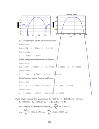
289. ωs2 =
2πFs2
FT
= 0.56π = 1.7593. Next using Eq. (7.26), we get ˆΩ p1 = tan
ωp1
2







 = 0.32492,
ˆΩ p2 = tan
ωp2
2







 = 4.1653, ˆΩ s1 = tan
ωs1
2





 = 0.77568,, and ˆΩ s2 = tan
ωs2
2





 =1.2088. The
stopband width is Bw = ˆΩ s2 − ˆΩ s1 = 0.43311. Now ˆΩ o
2
= ˆΩs2
ˆΩ s1 = 0.93764 and
ˆΩ p2
ˆΩ p1 = 1.3534 ≠ ˆΩ s2
ˆΩ s1. Hence we adjust the lower passband edge to
ˆΩ p1 =
ˆΩ s2
ˆΩ s1
ˆΩ p2
= 0.22511. Note ˆΩ o = 0.96832.
Analog bandstop filter specifications: ˆΩ p1 = 0.22511 radians, ˆΩ p2 = 4.1653 radians,
ˆΩ s1 = 0.41128 radians, ˆΩ s2 =1.2088 radians, αp = 2 dB, and αs = 40 dB.
(b) For the prototype analog lowpass filter we choose Ωs = 1. From Eq. (5.65) we then get
Ωp =
ˆΩ p1 ⋅Bw
ˆΩ o
2
− ˆΩ p1
2 =
0.22511× 0.43311
0.93764− 0.10557
= 0.16913.
Analog lowpass filter specifications: Ωs = 1 radians, Ωp = 0.16913 radians, αp = 2 dB, and αs
= 40 dB.
Code fragments used are:
[N,Wn] = buttord(0.16913, 1, 2, 40, 's');
[B,A] = butter(N, Wn,'s');
[BT,AT] = lp2bs(B,A,0.96832, 0.43311);
[num,den] = bilinear(BT,AT,0.5);
0 0.2 0.4 0.6 0.8 1
-30
-25
-20
-15
-10
-5
0
5
ω/π
(c) Analog lowpass transfer function coefficients:
Numerator
0 0 0 0.010001
Denominator
285

290. 1 0.43089 0.092835 0.010001
Analog bandstop transfer function coefficients:
Numerator
Columns 1 through 6
1 -1.5044e-16 2.8129 -2.8211e-16 2.6375 -1.3226e-16
Column 7
0.82435
Denominator
Columns 1 through 6
1 4.0206 10.895 15.664 10.216 3.5348
Column 7
0.82435
Digital bandstop transfer function coefficients:
Numerator
Columns 1 through 6
0.15762 -0.030434 0.47481 -0.060910 0.47481 -0.030434
Column 7
0.15762
Denominator
Columns 1 through 6
10 -0.094374 -0.0641472 -0.017232 0.33514 -0.010173
Column 7
-0.0061388
M7.13 The impulse response coefficients of the truncated FIR highpass filter with cutoff frequency
at 0.4π can be generated using the following MATLAB statements:
n = -M:M;
num = -0.4*sinc(0.4*n);
num(M+1) = 0.6;
The magnitude responses of the truncated FIR highpass filter for two values of M are shown
below:
286

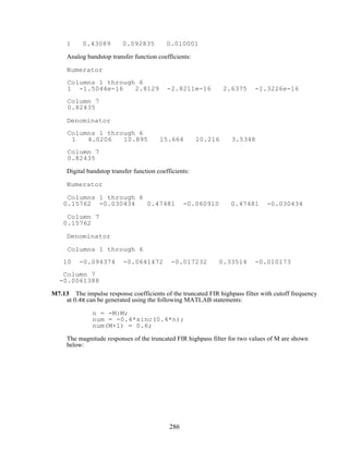
291. M7.14 The impulse response coefficients of the truncated FIR bandpass filter with cutoff frequencies
at 0.7π and 0.3π can be generated using the following MATLAB statements:
n = -M:M;
num = 0.7*sinc(0.7*n) - 0.3*sinc(0.3*n);
The magnitude responses of the truncated FIR bandpass filter for two values of M are shown
below:
M7.15 The impulse response coefficients of the truncated Hilbert transformer can be generated
using the following MATLAB statements:
n = 1:M;
c = 2*sin(pi*n/2).*sin(pi*n/2);b = c./(pi*n);
num = [-fliplr(b) 0 b];
The magnitude responses of the truncated Hilbert transformer for two values of M are shown
below:
287

292. M7.16 For notch filter design using the Hamming window, the following MATLAB program can be
used:
fc = input('Normalized notch angular frequency = ');
N = input('Desired notch filter order = ');% must be an even
integer
M = N/2;
n=-M:1:M;
t = fc*n;
lp = fc*sinc(t);
b = 2*[lp(1:M) (lp(M+1)-0.5) lp((M+2):N+1)];
bw = b.*hamming(N+1)';
[h2,w]=freqz(bw,1,512);
plot(w/pi,abs(h2));axis([0 1 0 1.2]);
xlabel('omega/pi');ylabel('Amplitude');
title(['omega = 'num2str(fc), ', Filter order =
',num2str(N)])
For a notch filter of length 41 with a notch frequency at 60-Hz and operating at a 400-Hz
sampling rate, the normalized angular notch frequency is given by ωo = 0.3π. The
magnitude response of the designed filter is shown below:
0 0.2 0.4 0.6 0.8 1
0
0.2
0.4
0.6
0.8
1
1.2
ω/π
ω = 0.3, Filter order = 40
M7.17 The desired function D(x) = 2.2x3
−3x2
+ 0.5 is defined for −3 ≤ x ≤ 3.5. We wish to
approximate D(x) by a quadratic function a2 x
2
+ a1 x+ a0 by minimizing the peak value of
288

293. the absolute error D(x)− a2 x
2
−a1 x− a0 . Since there are four unknowns a0, a1, a2 and ε ,
we need four extremal points on x in the range −3 ≤ x ≤ 3.5, which we arbitrarily choose as x1
= –3, x2 = –2, x3 = 1 and x4 = 3.5. We then solve the four linear equations
a0 + a1 xl + a2 xl
2
− (−1)
l
ε = D(xl ), l =1,2,3,4, which lead to
1 −3 9 1
1 −2 4 −1
1 1 1 1
1 3.5 1.225 −1










a0
a1
a2
ε












=
−85.9
−29.1
−0.3
−58.075










.
Its solution yields a0 = −1.6214, a1 = 18.229, a2 = −1.5857, and ε = −15.321. Figure (a) below
shows the plot of the error E1(x) = 2.2x3
− 1.4143x2
−18.229x + 2.1214 along with the values
of the error at the chosen extremal points.
The next set of extremal points are those points where E1(x) assumes its maximum absolute
values. These extremal points are given by x1 = –3, x2 = –1.454, x3 = 1.89 and x4 = 3.5. The
new values of the unknowns are obtained by solving
1 −3 9 1
1 −1.454 2.1141 −1
1 1.89 3.5721 1
1 3.5 1.225 −1










a0
a1
a2
ε












=
−85.9
−12.605
4.6365
5.8075










whose solution yields a0 = −7.0706, a1 = −17.021,, a2 = −1.3458, and ε = −18.857. Figure (b)
below shows the plot of the error E2(x) = 2.2x3
− 1.6542x2
−17.021x + 4.3685 along with the
values of the error at the chosen extremal points. This time the algorithm has converged as ε is
also the maximum value of the absolute error.
-2 0 2
-20
-10
0
10
20
x
-2 0 2
-20
-10
0
10
20
x
(a) (b)
M7.18 From Eqs. (7.7) and (7.8), the normalized bandedges are given by ωp = 0.2π and
ωs = 0.4π. Therefore, ωc = 0.3π and ∆ω = 0.2π.
(a) Using Eq. (7.77) and Table 7.2, the estimated order of the FIR filter for designing using
the Hamming window is given by N = 2M where M = 3.32π/∆ω = 16.6. We therefore
choose M = 17 or equivalently, N = 34. The MATLAB program used to generate the
windowed filter coefficients are
n = -17:17;
num = 0.4*sinc(0.4*n);
wh = hamming(35);
289

294. b = num.*wh';
0 10 20 30
-0.1
0
0.1
0.2
0.3
0.4
Time index n
Impulse Response Coefficients
0 0.2 0.4 0.6 0.8 1
-60
-40
-20
0
ω/π
Filter Designed Using Hamming Window
(b) For designing the FIR filter using the Hann window, we obtain from Eq. (7.77) and
Table 7.2, M = 3.11π/∆ω = 15.55. We choose M = 16, and hence N = 32.
0 10 20 30
-0.1
0
0.1
0.2
0.3
0.4
Time index n
Impulse Response Coefficients
0 0.2 0.4 0.6 0.8 1
-60
-40
-20
0
ω/π
Filter Designed Using Hann Window
(c) For designing the FIR filter using the Blackman window, we obtain from Eq. (7.77) and
Table 7.2, M = 5.56π/∆ω = 27.8. We choose M = 28, and hence N = 56.
0 10 20 30 40 50
-0.1
0
0.1
0.2
0.3
0.4
Time index n
Impulse Response Coefficients
0 0.2 0.4 0.6 0.8 1
-80
-60
-40
-20
0
ω/π
Filter Designed Using Blackman Window
The filter designed using the Hann window meets the specifications with a smaller length.
M7.19 From Eqs. (7.7) and (7.8), the normalized bandedges are given by ωp = 0.2π and
ωs = 0.4π. Therefore, ωc = 0.3π and ∆ω = 0.2π.
290

295. Substituting αs = 40 in Eq. (7.85) we obtain β = 3.3953. Next, substituting the value of
αs = 40 and ∆ω = 0.2π in Eq. (7.86) we obtain N = 22.289. We choose the next higher even
integer value of 24 as the filter order N, and hence M = 12. The code fragments used for the
design are given below:
n = -N/2:N/2;
num = 0.4*sinc(0.4*n);
wh = kaiser(N+1,3.3953);
b = num.*wh';
0 5 10 15 20 25
-0.1
0
0.1
0.2
0.3
0.4
Time index n
Impulse Response Coefficients
0 0.2 0.4 0.6 0.8 1
-60
-50
-40
-30
-20
-10
0
ω/π
M7.20 ωp = 0.3π , ωs = 0.5π , and αs = 40 dB. Thus, ωc =
ωp + ωs
2
= 0.4π, and
∆ω = ωs − ωp = 0.2π. From Table 7.2 we observe that Hann window is appropriate for the filter
design as it meets the minimum stopband attenuation requirement with a filter of lowest order.
From Eq. (7.77) and Table 7.2, we get M =
3.11π
∆ω
=
3.11π
0.2π
= 15.55. We choose M = 16
implying a filter of order N = 32.
Code fragments used in the design are given below:
n = -16:1:16;
lp = 0.4*sinc(0.4*n);
wh = hanning(33);
b = lp.*wh';
0 10 20 30
-0.1
0
0.1
0.2
0.3
0.4
Time index n
Impulse Response Coefficients
0 0.2 0.4 0.6 0.8 1
-60
-50
-40
-30
-20
-10
0
ω/π
Lowpass Filter Designed Using Hann Window
291

296. M7.21 ωp = 0.3π , ωs = 0.5π , and αs = 40 dB. Thus, ωc = 0.4π, and ∆ω = 0.2π. Using Eq. (7.82)
we estimate the filter order N = 2M which is given by N =
2.065× 40 − 16.4
2.285(0.2π)
= 45.859. Hence we
choose N = 46, i.e. M = 23.
Code fragments used for the design are:
n = -23:1:23;
lp = 0.4*sinc(0.4*n);
wh =chebwin(47,40);
b = lp.*wh';
0 0.2 0.4 0.6 0.8 1
-60
-50
-40
-30
-20
-10
0
ω/π
Filter Designed Using Dolph-Chebyshev Window
M7.22 Code fragments used for the design are:
n = -16:1:16;
b = fir1(32,0.4,hanning(33));
0 10 20 30
-0.1
0
0.1
0.2
0.3
0.4
Time index n
Impulse Response Coefficients
0 0.2 0.4 0.6 0.8 1
-60
-50
-40
-30
-20
-10
0
ω/π
Filter Designed Using fir1 with Hanning Window
M7.23 N = 29;
for k = 1:N+1
w = 2*pi*(k-1)/30;
if(w >= 0.5*pi & w <= 1.5*pi) H(k)= 1;
else H(k) = 0;
end
if(w <= pi) phase(k) = i*exp(-i*w*N/2);
else phase(k) = -i*exp(i*(2*pi-w)*N/2);
end
end
H = H.*phase;
292

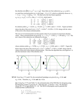
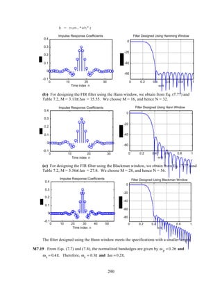
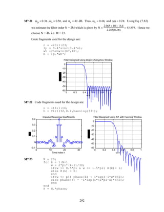
297. f = ifft(H);
[FF,w] = freqz(f,1,512);
k = 0:N;
subplot(211)
stem(k,real(f));
xlabel('Time index n'); ylabel('Amplitude')
subplot(212)
plot(w/pi,20*log10(abs(FF)));
xlabel('omega/pi'); ylabel('Gain, dB');
axis([0 1 -50 5]); grid on
0 10 20 30
-0.5
0
0.5
Time index n
0 0.2 0.4 0.6 0.8 1
-50
-40
-30
-20
-10
0
ω/π
M7.24 % Length = 41 and bandpass, hence Type 3 filter
N = 40; L = N+1;
for k = 1:L
w = 2*pi*(k-1)/L;
if (w >= 0.3*pi & w <= 0.5*pi) H(k) = i*exp(-
i*w*N/2);
elseif (w >= 1.5*pi & w <= 1.7*pi) H(k) =
-i*exp(i*(2*pi-w)*N/2);
else H(k) = 0;
end
end
f = ifft(H);
[FF,w] = freqz(f,1,512);
k = 0:N;
subplot(211);
stem(k,real(f));
xlabel('Time index n'); ylabel('h[n]');
subplot(212);
plot(w/pi,20*log10(abs(FF)));
ylabel(Gain, dB'); xlabel('omega/pi');
axis([0 1 -50 5]); grid;
293

298. 0 10 20 30 40
-0.2
-0.1
0
0.1
0.2
Time index n
0 0.2 0.4 0.6 0.8 1
-50
-40
-30
-20
-10
0
ω/π
M7.25 N=36; L=N+1;
for k = 0:36
if(k <= 5 | k>=32) H(k+1) = exp(-i*2*pi*k/L*18);
elseif (k == 6 | k == 31) H(k+1) = 0.5*exp(-
i*2*pi*k/L*18);
end
end
f = ifft(H);
[FF,w] = freqz(f,1,512);
k = 0:N;
subplot(211);
stem(k,real(f));axis([0 36 -0.1 0.4]);
xlabel('Time index n'); ylabel(h[n]);
subplot(212);
plot(w/pi,20*log10(abs(FF)));
xlabel('omega/pi'); ylabel('Gain, dB');
axis([0 1 -70 5]);grid;
0 10 20 30
-0.1
0
0.1
0.2
0.3
0.4
Time index n
0 0.2 0.4 0.6 0.8 1
-60
-40
-20
0
ω /π
M7.26 N = 36; L=N+1;
for k = 0:36
if(k <= 5 | k >= 32) H(k+1) = exp(-i*2*pi*k/L*18);
elseif (k ==6 | k == 31) H(k+1) = 2/3*exp(-i*2*pi*k/L*18);
elseif (k ==7 | k == 30) H(k+1) = 1/3*exp(-i*2*pi*k/L*18);
end
end
f = ifft(H);
[FF,w] = freqz(f,1,512);
k = 0:N;
294

299. subplot(211);
stem(k,real(f));
xlabel('Time index n'); ylabel('Amplitude');
subplot(212);
plot(w/pi,20*log10(abs(FF)));
xlabel('omega/pi'); ylabel(Gain, dB');
axis([0 1 -70 5]); grid;
0 10 20 30
-0.1
0
0.1
0.2
0.3
0.4
Time index n
0 0.2 0.4 0.6 0.8 1
-60
-40
-20
0
ω/π
M7.27 ωc = 0.3π and ∆ω = 0.2π.
(a) Hamming Window: From Exercise M7.18(a) we have M = 17. Code fragment used for
the design are:
b = fir1(2*M,0.3);
0 10 20 30 40
-0.1
0
0.1
0.2
0.3
Time index n
Impulse Response Coefficients
0 0.2 0.4 0.6 0.8 1
-60
-40
-20
0
ω/π
Filter Designed Using Hamming Window
(b) Hann Window: From Exercise M7.18(b) we have M = 16. Code fragment used for
the design are:
b = fir1(2*M,0.3, hanning(2*M+1));
295

300. 0 10 20 30
-0.1
0
0.1
0.2
0.3
0.4
Time index n
Impulse Response Coefficients
0 0.2 0.4 0.6 0.8 1
-60
-40
-20
0
ω/π
Filter Designed Using Hann Window
(c) Blackman Window: From Exercise M7.18(c) we have M = 28. Code fragment used for
the design are:
b = fir1(2*M,0.3, blackman(2*M+1));
0 10 20 30 40 50
-0.1
0
0.1
0.2
0.3
0.4
Time index n
Impulse Response Coefficients
0 0.2 0.4 0.6 0.8 1
-80
-60
-40
-20
0
ω/π
Filter Designed Using Blackman Window
(d) Kaiser Window: ωp = 0.2π , ωs = 0.4π , αs = 40 dB. Thus,
δs = 10−αs
/ 2
= 10−2
= 0.01. Code fragments used for the design are:
[N,Wn,beta,type] = kaiserord([0.2 0.4],[1 0], [0.01 0.01]);
b = fir1(N,0.3,kaiser(N+1,beta));
0 5 10 15 20
-0.1
0
0.1
0.2
0.3
0.4
Time index n
Impulse Response Coefficients
0 0.2 0.4 0.6 0.8 1
-60
-40
-20
0
ω/π
Filter Designed Using Kaiser Window
296

301. M7.28 ωp = 0.6π, ωs = 0.45π, αp = 0.2 dB and αs = 45 . Thus, ∆ω = 0.15π and
ωc =
0.6π + 0.45π
2
= 0.525π.
(a) Hamming Window: From Table 7.2 and Eq. (7.77) we have
M =
3.32π
∆ω
=
3.32π
0.15π
= 22.133, We choose M = 23, i.e. filter order N = 2M = 46.
Code fragment used is:
b = fir1(2*M,0.525,'high');
0 10 20 30 40
-0.4
-0.2
0
0.2
0.4
0.6
Time index n
Impulse Response Coefficients
0 0.2 0.4 0.6 0.8 1
-60
-40
-20
0
ω/π
Filter Designed Using Hammimg Window
(b) Hann Window: From Table 7.2 and Eq. (7.77) we have M =
3.11π
∆ω
=
3.11π
0.15π
= 20.733.
We choose M = 21, i.e. filter order N = 2M = 42.
Code fragment used is:
b = fir1(2*M,0.525,'high',hanning(2*M+1));
0 10 20 30 40
-0.4
-0.2
0
0.2
0.4
0.6
Time index n
Impulse Response Coefficients
0 0.2 0.4 0.6 0.8 1
-60
-40
-20
0
ω/π
Filter Designed Using Hann Window
(c) Blackman Window: From Table 7.2 and Eq. (7.77) we have
M =
5.56π
∆ω
=
5.56π
0.15π
= 37.067. We choose M = 38, i.e. filter order N = 2M = 76.
Code fragment used is:
297

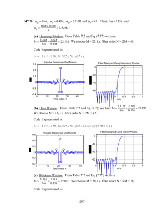
302. b = fir1(2*M,0.525,'high',blackman(2*M+1));
0 20 40 60
-0.4
-0.2
0
0.2
0.4
0.6
Time index n
Impulse Response Coefficients
0 0.2 0.4 0.6 0.8 1
-80
-60
-40
-20
0
ω/π
Filter Designed Using Blackman Window
(d) Kaiser Window: ωp = 0.6π , ωs = 0.45π , αs = 45 dB. Thus, ωc = 0.525π and
δs = 10−αs
/ 20
=10−2.25
= 0.0056234. Code fragments used for the design are:
ds = 0.0056234;
[N,Wn,beta,type]=kaiserord([0.45 0.6],[1 0],[ds ds]);
N = N+1;% For highpass filter, order must be even
b = fir1(N,0.525,'high',kaiser(N+1,beta));
0 10 20 30
-0.4
-0.2
0
0.2
0.4
0.6
Time index n
Impulse Response Coefficients
0 0.2 0.4 0.6 0.8 1
-80
-60
-40
-20
0
ω/π
Filter Designed Using Kaiser Window
M7.29 ωp1 = 0.55π , ωp2 = 0.7π , ωs1 = 0.45π , ωs2 = 0.8π , αp = 0.15 and αs = 40 . Thus,
∆ω1 = ωp1 − ωs1 = 0.1π and ∆ω2 = ωs2 − ωp2 = 0.1π = ∆ω1.
(a) Hamming Window: From Table 7.2 and Eq. (7.77) we have
M =
3.32π
∆ω1
=
3.32π
0.1π
= 33.2 We choose M = 34, i.e. filter order N = 2M = 68.
Code fragment used is:
b = fir1(2*M,[0.5 0.75]);
298

303. 0 20 40 60
-0.2
-0.1
0
0.1
0.2
0.3
Time index n
Impulse Response Coefficients
0 0.2 0.4 0.6 0.8 1
-60
-40
-20
0
ω/π
Filter Designed Using Hamming Window
(b) Hann Window: From Table 7.2 and Eq. (7.77) we have M =
3.11π
∆ω
=
3.11π
0.1π
= 31.1.
We choose M = 32, i.e. filter order N = 2M = 64.
Code fragment used is:
b = fir1(2*M,[0.5 0.75],hanning(2*M+1));
0 20 40 60
-0.2
-0.1
0
0.1
0.2
0.3
Time index n
Impulse Response Coefficients
0 0.2 0.4 0.6 0.8 1
-60
-40
-20
0
ω/π
Filter Designed Using Hann Window
(c) Blackman Window: From Table 7.2 and Eq. (7.77) we have
M =
5.56π
∆ω1
=
5.56π
0.1π
= 55.6. We choose M = 56, i.e. filter order N = 2M = 12.
ωc1 =
ωp1 + ωs1
2
=
0.55π + 0.45π
2
= 0.5π and ωc2 =
ωp2 + ωs2
2
=
0.7π + 0.8π
2
= 0.75π.
Code fragment used is:
b = fir1(2*M,[0.55 0.7],blackman(2*M+1));
299

304. 0 20 40 60 80 100
-0.1
0
0.1
0.2
Time index n
Impulse Response Coefficients
0 0.2 0.4 0.6 0.8 1
-80
-60
-40
-20
0
ω/π
Filter Designed Using Blackman Window
(d) Kaiser Window: ωp1 = 0.55π , ωp2 = 0.7π , ωs1 = 0.45π , ωs2 = 0.8π , αp = 0.15 and
αs = 40 . Thus, δp = 10−αp
/ 20
=10−0.075
= 0.98288 and δs = 10−αs
/ 20
=10−2
= 0.01.
Code fragments used for the design are:
[N,Wn,beta,type]= kaiserord([0.55 0.7],[1 0],[0.98288 0.01]);
b = fir1(N,[0.5 0.75],kaiser(N+1,beta));
0 10 20 30
-0.2
-0.1
0
0.1
0.2
0.3
Time index n
Impulse Response Coefficients
0 0.2 0.4 0.6 0.8 1
-60
-40
-20
0
ω/π
Filter Designed Using Kaiser Window
M7.30 From Eq. (7.7), the normalized crossover frequency ωc =
2π ×10
80
= 0.25π The delay-
complementary FIR lowpass and highpass filter coefficients of length 27 are then generated
using the MATLAB statements:
d1 = fir1(26,0.7854);
d2 = -d1;d2(14) = 1 - d1(14);
The gain responses of the two filters are as indicated below:
300

305. 0 0.2 0.4 0.6 0.8 1
-60
-40
-20
0
ω/π
H
LP
(z)H
HP
(z)
M7.31 The filter coefficients of the FIR lowpass and the highpass, and their delay-complementary
FIR bandpass filter are generated using the MATLAB program:
c = hanning(31);
d1 = fir1(30,0.15873,c);
d2 = fir1(30,0.40816,'high',c);
d3 = -d1-d2;d3(16) = 1 - d1(16) - d2(16);
The gain responses of the three FIR filters are as given below:
0 0.2 0.4 0.6 0.8 1
-60
-40
-20
0
20
ω/π
HLP
(z) HBP
(z) HHP
(z)
M7.32 The filter coefficients are generated using the MATLAB program:
fpts = [0 0.4 0.42 0.7 0.721 1];
mval = [0.5 0.5 0.3 0.3 1.0 1.0];
b = fir2(80,fpts,mval);
The gain response of the multiband FIR filter is as given below:
301

306. 0 0.2 0.4 0.6 0.8 1
0.2
0.4
0.6
0.8
1
1.2
ω/π
M7.33 The filter was also designed by using remezord to estimate the filter order and then using
remez to determine the filter coefficients. To this end the MATLAB program used is given
below:
Rp = 0.1; Rs = 40; FT = 20;
f = [2 4]; m = [1 0];
dev = [(10^(Rp/20) -1)/(10^(Rp/20) +1) 10^(-Rs/20)];
[N, fo, mo, wo] = remezord(f, m, dev, FT);
b = remez(N,fo,mo,wo);
The filter obtained using the above program is of length 20, but its gain response did not meet
the specifications. The specifications were met when the filter order was increased to 22.
0 0.2 0.4 0.6 0.8 1
-60
-40
-20
0
ω/π
M7.34 The filter was also designed by using remezord to estimate the filter order and then using
remez to determine the filter coefficients. To this end the MATLAB program used is given
below:
Rp = 0.2; Rs = 45;
f = [0.45 0.65]; m = [1 0];
dev = [(10^(Rp/20) -1)/(10^(Rp/20) +1) 10^(-Rs/20)];
[N, fo, mo, wo] = remezord(f, m, dev);
b = remez(N,fo,mo,wo);
The filter obtained using the above program is of length 27, but its gain response did not
meet the specifications. The specifications were met when the filter order was increased to 30.
302

307. 0 0.2 0.4 0.6 0.8 1
-60
-40
-20
0
ω/π
M7.35 The code fragments used to design the FIR bandpass filter are:
Rp = 0.15; Rs = 40;
f = [0.45 0.55 0.7 0.8]; m = [0 1 0];
dev = [10^(-Rs/20) (10^(Rp/20) -1)/(10^(Rp/20) +1) 10^(-
Rs/20)];
[N, fo, mo, wo] = remezord(f, m, dev);
b = remez(N,fo,mo,wo);
The filter obtained using the above program is of length 40, but its gain response did not
meet the specifications. The specifications were met when the filter order was increased to 41.
0 0.2 0.4 0.6 0.8 1
-60
-40
-20
0
ω/π
M7.36 The code fragment used to design a length-32 differentiator is given below.
b = remez(31,[0 1],[0 pi],'differentiator');
The magnitude response of the differentiator designed is shown below:
303

308. 0 0.2 0.4 0.6 0.8 1
0
0.5
1
1.5
2
2.5
3
ω/π
M7.37 The code fragments used to design the 26-th order Hilbert transformer are:
f = [0.01 0.078 0.08 0.92 0.94 1];
m = [0 0 1 1 0 0];
wt = [1 60 1];
b = remez(28,f,m,wt,'hilbert');
Note that the passband and the stopbands have been weighted to reduce the ripple in the
passband. The magnitude response of the Hilbert transformer designed is shown below:
0 0.2 0.4 0.6 0.8 1
0
0.2
0.4
0.6
0.8
1
ω/π
M7.38 The code fragment used for the design is
b = firls(31,[0 0.9],[0 0.9*pi],'differentiator');
0 0.2 0.4 0.6 0.8 1
0
0.5
1
1.5
2
2.5
3
ω/π
304

309. M7.39 From the given specifications
ωs
M
= 0.2π . We also require
ωs
M
≤
2π − ωs
M
, for no overlap to
occur in H(ejMω
) (see Figure P7.3(b) ). Hence 0.2π ≤
2π
M
− 0.2π which implies M ≤ 5.
We choose M = 4. Hence specifications for H(z) are ωp = 0.6π , ωs = 0.8π, δp = 0.001 and
δs = 0.001. Substituting these values in Eq. (7.15), we arrive at the estimated value of the
FIR filter length as N = 33.
Specifications for F(z) are ωp = 0.15π, ωs = 0.3π , δp = 0.001 and δs = 0.001. Hence, from
Eq. (7.15), the estimated length of F(z) is N = 43.
Therefore the total number of multiplications required per output sample is
33
2
+ 43( )×
1
2
=
30. (The division by 2 is due to the fact that H(z) and F(z) are linear phase filters. )
On the other hand for a direct single stage implementation, we note that the specifications of
G(z) are: wp = 0.15π, ws = 0.2π, dp = 0.002, ds = 0.001. Hence, the filter length of G(z)
from Eq. (7.15) is 121. Therefore the total number of multiplications required per output
sample is 121/2 = 61.
0 0.2 0.4 0.6 0.8 1
-60
-40
-20
0
20
ω/π
H(zM
)F(z)
0 0.2 0.4 0.6 0.8 1
-60
-40
-20
0
ω/π
G(z)
M7.40 From the specified stopband edge ωs = 0.14π, we get the estimated order N pf the RRS
prefilter H(z) as N ≅
2π
ωs
=14.2857. We choose N = 15. Next using the following two
MATLAB functions we design the equalizer F(z) and the overall cascaded filter H(z)F(z).
% Plotting function
% plots the result of using an equalizer of length InpN
function[N] = plotfunc(InpN) ;
% Creating filters
Wfilt = ones(1,InpN);
Efilt = remezfunc(InpN, Wfilt);
% Plot running sum filter response
%figure(1)
Wfilt = Wfilt/sum(Wfilt);
[hh,w]=freqz(Wfilt,1,512);
plot(w/pi,20*log10(abs(hh)));
axis([0 1 -50 5]); grid;
xlabel('omega/pi'); ylabel('Gain, dB');
title('Prefilter H(z)');
305

310. % Plot equalizer filter response
%figure(2)
pause
[hw,w]=freqz(Efilt,1,512);
plot(w/pi,20*log10(abs(hw)));
axis([0 1 -50 5]); grid;
xlabel('omega/pi'); ylabel('Gain, dB');
title('Equalizer F(z)');
% Plot cascaded filter response
%figure(3)
pause
Cfilt = conv(Wfilt, Efilt);
[hc,w]=freqz(Cfilt,1,512);
plot(w/pi,20*log10(abs(hc)));
axis([0 1 -80 5]); grid;
title('Cascaded filter H(z)F(z)');
ylabel('G(omega), dB'); xlabel('omega/pi');
% Plot filter coefficients
%figure(4)
pause
%subplot(2,1,1);
n1 = 0:length(Wfilt)-1;
stem(n1,Wfilt);
xlabel('Time index n');ylabel('Amplitude');
title('Prefilter coefficients');
pause
%subplot(2,1,2);
n2 = 0:length(Efilt)-1;
stem(n2,Efilt);
xlabel('Time index n');ylabel('Amplitude');
title('Equalizer coefficients');
% Remez function using 1/P(z) as desired amplitude
% and P(z) as weighting
function [N] = remezfunc(Nin, Wfilt);
% Nin : number of tuples in the remez equalizer filter
% Wfilt : the prefilter
a = [0:0.001:0.999]; % The accuracy of the computation
w = a.*pi;
wp = 0.042*pi; % The passband edge
ws = 0.14*pi; % The stopband edge
i = 1;
n = 1;
for t = 1 : (length(a)/2)
if w(2*t) < wp
pas(i) = w(2*t - 1);
pas(i+1) = w(2*t);
i = i + 2;
end;
if w(2*t-1) > ws
sto(n) = w(2*t-1);
sto(n+1) = w(2*t);
n = n + 2;
end;
end;
w = cat(2, pas, sto);
bi = length(w)/2; % bi gives the number of subintervals
for t1 = 1:bi
306

311. bw(t1) = (w(2*t1) + w(2*t1-1))/2;
W(t1) = Weight(bw(t1), Wfilt,ws);
end;
W = W/max(W);
for t2 = 1:length(w)
G(t2) = Hdr(w(t2), Wfilt, wp);
end;
G = G/max(G);
N = remez(Nin, w/pi, G, W);
% Weighting function
function[Wout] = Weight (w, Wfilt, ws);
K = 22.8;
L = length(Wfilt);
Wtemp = 0;
Wsum = 0;
for k = 1:L
Wtemp = Wfilt(k)*exp((k-1)*i*w);
Wsum = Wsum + Wtemp;
end;
Wout = abs(Wsum);
if w > ws
Wout = K*max(Wout);
end;
% Desired function
function[Wout] = Hdr (w, Wfilt, ws);
if w <= ws
L = length(Wfilt);
Wtemp = 0;
Wsum = 0;
for k = 1:L
Wtemp = Wfilt(k)*exp(i*(k-1)*w);
Wsum = Wsum + Wtemp;
end;
Wsum = abs(Wsum);
Wout = 1/Wsum;
else Wout = 0;
end;
0 0.2 0.4 0.6 0.8 1
-50
-40
-30
-20
-10
0
ω/π
Prefilter H(z)
0 0.2 0.4 0.6 0.8 1
-50
-40
-30
-20
-10
0
ω /π
Equalizer F(z)
307

312. 0 0.2 0.4 0.6 0.8 1
-80
-60
-40
-20
0
Cascaded filter H(z)F(z)
ω/π
0 5 10 15
0
0.02
0.04
0.06
0.08
Time index n
Prefilter coefficients
0 5 10 15
0
0.02
0.04
0.06
0.08
0.1
Time index n
Equalizer coefficients
308

313. Chapter 8 (2e)
8.1
z–1
z–1
z–1
–1
–1
α0
α1
α2
α3
β1
β2
β3
x[n] y[n]
w5[n]
w4[n]
w3[n]
w2 [n]
w1[n]
Analysis yields w1[n]= α1 β1 w1[n −1]+ x[n]− w3[n],
w2[n] = β3w4[n −1],
w3[n]= β2w5[n −1],
w4[n] = α3w2[n]+ w3[n],
w5[n] = α2w3[n]− w2[n]+ β1 w1[n −1],
y[n] = α0x[n]+ β1 w1[n −1].
In matrix form the above set of equations is given by:
w1[n]
w2
[n]
w3
[n]
w4[n]
w5[n]
y[n]


















=
0 0 −1 0 0 0
0 0 0 0 0 0
0 0 0 0 0 0
0 α3
1 0 0 0
0 −1 α2 0 0 0
0 0 0 0 0 0
















w1[n]
w2
[n]
w3
[n]
w4[n]
w5[n]
y[n]


















+
α1β1 0 0 0 0 0
0 0 0 β3
0 0
0 0 0 0 β2
0
0 0 0 0 0 0
β1 0 0 0 0 0
β1 0 0 0 0 0


















w1[n −1]
w2
[n −1]
w3
[n −1]
w4[n −1]
w5[n −1]
y[n −1]


















+
x[n]
0
0
0
0
α0 x[n]
















Here the F matrix is given by
F =
0 0 −1 0 0 0
0 0 0 0 0 0
0 0 0 0 0 0
0 α3
1 0 0 0
0 −1 α2 0 0 0
0 0 0 0 0 0
















Since the F matrix contains nonzero entries above the main diagonal, the above set of equations
are not computable.
8.2 A computable set of equations of the structure of Figure P8.1 is given by
w2[n] = β3 w4[n −1],
w3[n]= β2 w5[n −1],
309

314. w1[n]= α1β1 w1[n −1]− w3[n]+ x[n],
w4[n] = α3w2[n]+ w3[n],
w5[n] = α2w3[n]− w2[n]+ β1 w1[n −1],
y[n] = α0x[n]+ β1 w1[n −1].
In matrix form the above set of equations is given by:
w2[n]
w3
[n]
w1[n]
w4[n]
w5[n]
y[n]


















=
0 0 0 0 0 0
0 0 0 0 0 0
0 −1 0 0 0 0
α3
1 0 0 0 0
−1 α2 0 0 0 0
0 0 0 0 0 0
















w2[n]
w3
[n]
w1[n]
w4[n]
w5[n]
y[n]


















+
0 0 0 β3 0 0
0 0 0 0 β2 0
0 0 α1
β1
0 0 0
0 0 0 0 0 0
0 0 β1 0 0 0
0 0 β1 0 0 0


















w1[n −1]
w2
[n −1]
w3
[n −1]
w4[n −1]
w5[n −1]
y[n −1]


















+
0
0
x[n]
0
0
α0 x[n]
















Here the F matrix is given by
F =
0 0 0 0 0 0
0 0 0 0 0 0
0 −1 0 0 0 0
α3
1 0 0 0 0
−1 α2 0 0 0 0
0 0 0 0 0 0
















Since the F matrix does not contain nonzero entries above the main diagonal, the new set of
equations are computable.
8.3
z–1
z–1
z–1
–1
α0
α1
α2
α3
β1
β2
β3
x[n] y[n]
w5[n]
w4[n]
w3[n]
w2[n]
w1[n]
w6
[n]
–1
Analysis yields w1[n]= x[n]− α2 w3[n]+ w2[n],
w2[n] = α1 β1w1[n −1],
w3[n]= α1 w1[n]− α3 w5[n]+ w4[n],
w4[n] = α2 β2w3[n −1],
w5[n] = α2 w3[n]+ w6[n],
w6[n] = α3 β3w5[n− 1],
310

315. y[n] = α0x[n]+ α1w1[n].
In matrix form
w1
[n]
w2[n]
w3[n]
w4
[n]
w5
[n]
w6[n]
y[n]




















=
0 1 −α2 0 0 0 0
0 0 0 0 0 0 0
α1 0 0 1 −α3 0 0
0 0 0 0 0 0 0
0 0 α2
0 0 0 1
0 0 0 0 0 0 0
α1 0 0 0 0 0 0




















w1
[n]
w2[n]
w3[n]
w4
[n]
w5
[n]
w6[n]
y[n]




















+
0 0 0 0 0 0 0
α1β1 0 0 0 0 0 0
0 0 0 0 0 0 0
0 0 α2β2 0 0 0 0
0 0 0 0 0 0 0
0 0 0 0 α3
β3
0 0
0 0 0 0 0 0 0




















w1
[n −1]
w2[n−1]
w3[n −1]
w4
[n− 1]
w5
[n −1]
w6[n −1]
y[n −1]




















+
x[n]
0
0
0
0
0
α0
x[n]


















Here the F matrix is given by F =
0 1 −α2 0 0 0 0
0 0 0 0 0 0 0
α1 0 0 1 −α3 0 0
0 0 0 0 0 0 0
0 0 α2
0 0 0 1
0 0 0 0 0 0 0
α1 0 0 0 0 0 0




















Since the F matrix contains nonzero entries above the main diagonal, the above set of equations
are not computable.
8.4 The signal-flow graph representation of the structure of Figure P8.1 is shown below:
x[n] y[n]
w1[n]
v1[n]
w2[n]
w3[n]
w4[n]w5[ n]
1
1
1 1
α1 α2 α3
α0
β2z
−1β1z
−1
β3z
−1
−1
−1
The reduced signal-flow graph obtained by removing the branches going out of the input node
and the delay branches is as indicated below:
311

316. y[n]
w1[n]
v1[n]
w2[n]
w3[n]
w4[n]w5[n]
1
1 1
α1 α2 α3
−1
−1
From the above signal-flow graph we arrive at its precedence graph shown below:
−1
y[n]
w1[n]v1[n]
w2[n]
w3[n] w4[n]
w5[n]
α1
1
1
α2
1
α3
−1
1
N
2
N
In the above precedence graph, the set N 1 contains nodes with only outgoing branches and
the final set N 2 contains nodes with only incoming branches. As a result, the structure of
Figure P8.1 has no delay-free loops. A valid computational algorithm by computing the
node variables in set N 1 first in any order followed by computing the node variables in set
N 2 in any order. For example, one valid computational algorithm is given by
v1[n] = β1 w1[n −1],
w3[n]= β2 w5[n −1],
w2[n] = β3 w4[n −1],
w1[n]= α1 v1[n]− w3[n]+ x[n],
w4[n] = α3 w2[n]+ w3[n],
w5[n] = α2 w3[n]− w2[n]+ β1 v1[n],
y[n] = α0 x[n]+ v1[n].
8.5 The reduced signal-flow graph obtained by removing the branches going out of the input node
and the delay branches from the signal-flow graph representation of the structure of Figure
P8.2 is as indicated below:
312

317. α2
y[n]w1[n]
w2[n]
w3[n]
w4[n]
w5[n]
α1
w6[n]
α1
–α3
1
–α2
The only node with outgoing branch is w6[n] and hence it is the only member of the set N 1.
Since it is not possible to find a set of nodes N 2 with incoming branches from N 1 and all
other branches being outgoing, the structure of Figure P8.2 has delay-free loops and is
therefore not realizable.
8.6 (a)
− k3
k3
− k2
k2
− k1
k1
z−1 z−1 z−1
w3[n] w2[n] w1[n]
s2[n]s3[n]
↑↑
x[n]
y[n]
Analysis of Figure P8.3 yields w1[n]= w2[n]− k1w1[n −1],
w2[n] = w3[n]− k2s2[n −1],
w3[n]= x[n]− k3s3[n− 1],
s2[n] = k1w1[n]+ w1[n −1],
s3[n]= k2w2[n]+ s2[n −1],
y[n] = k3w3[n]+ s3[n− 1].
In matrix form we have
w1[n]
w2
[n]
w3
[n]
s2[n]
s3[n]
y[n]


















=
0
0
x[n]
0
0
0
















+
0 1 0 0 0 0
0 0 1 0 0 0
0 0 0 0 0 0
k1
0 0 0 0 0
0 k2 0 0 0 0
0 0 k3 0 0 0
















F
1 244444 344444
w1[n]
w2
[n]
w3
[n]
s2[n]
s3[n]
y[n]


















+
−k1
0 0 0 0 0
0 0 0 −k2 0 0
0 0 0 0 −k3 0
1 0 0 0 0 0
0 0 0 1 0 0
0 0 0 0 1 0
















G
1 244444 344444
w1[n −1]
w2
[n −1]
w3
[n −1]
s2[n −1]
s3[n −1]
y[n −1]


















As the diagonal elements of the F-matrix are all zeros, there are no delay-free loops.
However, the set of equations as ordered is not computable as there non-zero elements above
the diagonal of F.
(b) The reduced signal flow-graph representation of the structure of Figure P8.3 is shown
below:
313

318. w3[n]
w 2[n]
w1[n] s2[n]
s3[n] y[n]
k1
k2
k3
1
1
From the above flow-graph we observe that the set composed of nodes with out going branches
is N1 = w3[n]{ }. The set composed of nodes with out going branches and incoming branches
from N1 is N 2 = w2[n]{ }. The set composed of nodes with out going branches and incoming
branches from N1 and N 2 is N3 = w1[n]{ }. Finally, set composed of nodes with only
incoming branches from N1 , N 2 and N3 is N 4 = s2[n], s3[n], y[n]{ }. Therefore, one
possible ordered set of equations that is computable is given by
w3[n]
w2
[n]
w1[n]
s2[n]
s3[n]
y[n]


















=
0
0
x[n]
0
0
0
















+
0 0 0 0 0 0
1 0 0 0 0 0
0 1 0 0 0 0
0 0 k1
0 0 0
0 k2 0 0 0 0
k3 0 0 0 0 0
















F
1 244444 344444
w3[n]
w2
[n]
w1[n]
s2[n]
s3[n]
y[n]


















+
0 0 0 0 −k3
0
0 0 0 −k2 0 0
0 0 −k3 0 0 0
0 0 1 0 0 0
0 0 0 1 0 0
0 0 0 0 1 0
















G
1 2444444 3444444
w3[n −1]
w2
[n −1]
w1[n −1]
s2[n −1]
s3[n −1]
y[n −1]


















Note that all elements on the diagonal and above doagonal are zeros.
8.7 H(z) =
p0 + p1z−1 + p2z−2
1−3z−1 − 5z−2 and h[n]{ } = 2.1, 1.1, −3.2, −4.1, −28.3, L{ }, n = 0,1,K
From Eq. (8.15) we have
p0
p1
p2










=
2.1 0 0
1.1 2.1 0
−3.2 1.1 2.1








1
−3
−5








=
2.1
−5.2
−17








. Hence,
P(z) = 2.1− 5.2z−1
− 17z−2
.
8.8 H(z) =
p0 + p1z−1 + p2z−2
1+ d1
z−1 + d2
z−2 and h[n]{ } = 3, −2, −6, 12, −15{ }, 0 ≤ n ≤ 4. The equation
corresponding to Eq. (8.12) is
p0
p1
p2
0
0














=
3 0 0
−2 3 0
−6 −2 3
12 −6 −2
−15 12 −6












1
d1
d2










. Therefore, from EQ. (8.17) we
314

319. have
d1
d2





 = −
−6 −2
12 −6




−1
12
−15



 =
1.7
0.9



, and from Eq. (8.18) we have
p0
p1
p2










=
3 0 0
−2 3 0
−6 −2 3








1
1.7
0.9








=
3
3.1
−6.7








. Hence, H(z) =
3+ 3.1z−1
− 6.7z−2
1+ 1.7z−1 + 0.9z−2 .
8.9 H(z) =
p0 + p1z−1 + p2z−2 + p3z−3
1+ d1
z−1 + d2
z−2 + d3
z−3 and
h[n]{ } = 2, −5, 6, −2, −9, 18, −7 −31, 65, −30, L{ }, n ≥ 0. The equation
corresponding to Eq. (8.17) is given by
p0
p1
p2
p3
0
0
0




















=
2 0 0 0
−5 2 0 0
6 −5 2 0
−2 6 −5 2
−9 −2 6 −5
18 −9 −2 6
−7 18 −9 −2


















1
d1
d2
d3












. Therefore, from Eq.
(8.17) we have
d1
d2
d3










= −
−2 6 −5
−9 −2 6
18 −9 −2








−1
−9
18
−7








=
2
3
1








and from Eq. (8.18) we have
p0
p1
p2
p3












=
2 0 0 0
−5 2 0 0
6 −5 2 0
−2 6 −5 2










1
2
3
1










=
2
−1
2
−3










. Hence, H(z) =
2− z−1
+ 2z−2
− 3z−3
1+ 2z−1 + 3z−2 + z−3 .
8.10 G(z) =
p0 + p1z−1 + p2 z−2 + p3 z−3
2 − 6z−1 + 8z−2 +10z−3 with g[n]= 3, 7, 13, −3{ }, 0 ≤ n ≤ 3. Therefore, from
Eq. (8.18) we have
p0
p1
p2
p3












=
3 0 0 0
7 3 0 0
13 7 3 0
−3 13 7 3










2
−6
8
10










=
6
−4
8
2










. Hence, G(z) =
6− 4z−1
+ 8z−2
+ 2z−3
2 − 6z−1 + 8z−2 +10 z−3 .
8.11 H(z) =
p0 + p1z−1 + p2 z−2 + p3 z−3 + p4 z−4
1+ 2z−1 + 2z−2 + 3z−3 + 3z−4 with
h[n]{ } = 2, 0, −5, −10, −10, 55, −45, 40, −125, 140, −15{ } 0 ≤ n ≤10
The equation corresponding to Eq. (8.18) is given by
p0
p1
p2
p3
p4
















=
2 0 0 0 0
0 2 0 0 0
−5 0 2 0 0
−10 −5 0 2 0
−10 −10 −5 0 2












1
2
2
3
3












=
2
4
−1
−14
−34












.
Therefore, H(z) =
2+ 4z−1
− z−2
−14 z−3
− 34 z−4
1+ 2z−1 + 2z−2 + 3z−3 + 3z−4 .
315

320. 8.12 The k-th sample of an N-point DFT is given by X[k]= x[n]WN
nk
k =0
N−1
∑ . Thus the computation of
X[k] requires N complex multiplications and N–1 complex additions. Now each complex
multiplication, in turn, requires 4 real multiplications, and 2 real additions. Likewise, each
complex addition requires 2 real additions. As a result, the N complex multiplications needed
to compute X[k] require a total of 4N real multiplications and a total of 2N real additions.
Similarly, the N–1 complex additions needed in the computation of X[k] require a total of
2N–2 real additions. Hence, each sample of the N-point DFT involves 4N real multiplications
and 4N–2 real additions. The computation of all N DFT samples thus requires 4N2 real
multiplications and (4N–2)N real additions.
8.13 Let the two complex numbers be α = a + jb and β = c + jd. Then, αβ = (a + jb)(c + jd)
= (ac – bd)+ j(ad+ bc) which requires 4 real multiplications and 2 real additions. Consider the
products (a + b)(c + d), ac and bd which require 3 real multiplications and 2 real additions.
The imaginary part of αβ can be formed from (a + b)(c + d)− a c – bd = a d + bc which
now requires 2 real additions. Likewise, the real part of αβ can be formed by forming ac – bd
requiring an additional real addition. Hence, the complex multplication αβ can be computed
using 3 real multplications and 5 real additions.
8.14 The center frequency of bin k: fc(k) =
kFT
N
where N = # of bins, and FT is the sampling
frequency. Inverting we have k(f) =
f N
FT








. Therefore, the absolute difference from one of the
given four tones (150 Hz, 375 Hz, 620 Hz, and 850 Hz) to the center of its bin is given by
dist(N,f) = f −
FT
N
f N
FT








. It follows from this equation that the distance goes to zero if
FT
N
f N
FT








= f or
f N
FT
is an integer.
The total distance is reduced to zero if
fiN
FT
is an integer for i = 1,K,4. The minimum N for
which this is true is 500.
However, the total distance can be small, but nonzero, for significantly smaller values of N. The
MATLAB generated plot given below shows a nice minimum at N = 21.
5 10 15 20 25 30 35
0
200
400
600
800
Number of bins (N)
Total absolute difference plot
316

321. 8.15
z
–1
WN
–k
y[n]
y[–1] = 0
x[n]
Hk (z) =
1
1− WN
−k
z
−1 . Hence, Y(z) =
X(z)
1− WN
−k
z
−1 =
1+ z
–N / 2
1− WN
−k
z
−1 .
For k = 1, Y(z) =
1+ z
–N / 2
1− WN
−1
z
−1 = (1+ z
–N / 2
)(1+ WN
−1
z
−1
+ WN
−2
z
−2
+L+ WN
−N / 2
z
−N / 2
+L
Hence, y[n] = 1, WN
−1
, WN
−2
,L,WN
−(N−2) / 2
,1+ WN
−N / 2
,L,1+ WN
−(N −1)
,L{ }
For k = N/2, Y(z) =
1+ z
– N / 2
1− WN
−N / 2
z
−1 . Hence,
y[n] = 1, −1, 1, −1, K −1, 2, 0, 2, 0, K 0{ }
8.16
WN
2
x[0]
x[2]
x[4]
x[6]
x[1]
x[3]
x[5]
x[7]
X[0]
X[1]
X[2]
X[3]
X[5]
X[6]
X[7]
X[4]
WN
0
WN
0
WN
0
WN
0
WN
0
WN
0
WN
0
WN
2
WN
2
WN
2
WN
1
WN
3
–1
–1
–1
–1
–1
–1
–1
–1
–1
–1
–1
–1
8.17
317

322. x[0]
x[2]
x[4]
x[6]
x[1]
x[3]
x[5]
x[7]
X[0]
X[1]
X[2]
X[3]
X[5]
X[6]
X[7]
X[4]
WN
0
WN
0
WN
0
WN
0
WN
0
WN
0
WN
0
WN
2
WN
2
WN
2
WN
1
WN
3
–1
–1
–1
–1
–1
–1
–1
–1
–1
–1
–1
–1
8.18 X[k]= x[n]WN
nk
n =0
N−1
∑
= x[nr1]WN
nkr1
n =0
N
r1
−1
∑ + x[nr1 +1]WN
nkr1+k
n=0
N
r1
−1
∑ +L + x[nr1 + r1 − 1]WN
nkr1+(r1−1)k
n=0
N
r1
−1
∑
= x[nr1 + i]WN
nkr1
(N / r1
)−point DFT
1 244 344
n=0
N
r1
−1
∑
i =0
r1−1
∑ ⋅WN
ki
Thus, if the (N/r1)-point DFT has been calculated, we need at the first stage an additional
(r1 – 1) multiplications to compute one sample the N-point DFT X[k] and as a result, additional
(r1 – 1)N multiplications are required to compute all N samples of the N-point DFT.
Decomposing it further, it follows then that additional (r2 – 1)N multiplications are needed at
the second stage, and so on. Therefore,
Total number of multiply (add) operations = (r1 – 1)N + (r2 – 1)N + . . . + (rν – 1)N
= ri − ν
i=1
ν
∑





 N.
8.19 X(z) = X0 (z
3
) + z
−1
X1(z
3
) + z
−2
X2(z
3
). Thus, the N-point DFT can be expressed as
X[k]= X0[< k >N / 3]+ WN
k
X1[< k >N / 3]+ WN
2k
X2[< k >N / 3]. Hence, the structural
interpretation of the first stage of the radix-3 DFT is as indicated below:
318

323. X[k]x[n]
z
x0[n]
x1[n] WN
k
z
3
3
3
X0[< k > N
3
]
X1[< k > N
3
]
X2[< k > N
3
]
x2[n]
N
3
−point
DFT
N
3
−point
DFT
N
3
−point
DFT
WN
2k
8.20 X[k]= x[n]W9
nk
n=0
8
∑ = x[0]W9
0⋅k
+ x[3]W9
3k
+ x[6]W9
6k
( )
+ x[1]W9
k
+ x[4]W9
4k
+ x[7]W9
7k
( )+ x[2]W9
2k
+ x[5]W9
5k
+ x[8]W9
8k
( )
= x[0]W3
0⋅k
+ x[3]W3
k
+ x[6]W3
2k
( )+ x[1]W3
0⋅k
+ x[4]W3
k
+ x[7]W3
2k
( )W9
k
+ x[2]W3
0⋅k
+ x[5]W3
k
+ x[8]W3
2k
( )W9
2k
= G0[< k >3]+ G1[< k >3 ]W9
k
+ G2[< k >3]W9
2k
,
where G0[< k >3] = x[0]W3
0⋅k
+ x[3]W3
k
+ x[6]W3
2k
, G1[< k >3 ]= x[1]W3
0⋅k
+ x[4]W3
k
+ x[7]W3
2k
,
and G2[< k >3] = x[2]W3
0⋅k
+ x[5]W3
k
+ x[8]W3
2k
, are three 3-point DFTs. A flow-graph
representation of this DIT mixed-radix DFT computation scheme is shown below:
x[0]
x[2]
x[4]
x[6]
x[1]
x[3]
x[5]
x[7]
x[8]
X[0]
X[1]
X[2]
X[3]
X[5]
X[6]
X[7]
X[4]
X[8]
3-point
DFT
3-point
DFT
3-point
DFT
G0[0]
G0[1]
G0[2]
G1[2]
G1[1]
G1[ 0]
G2[0]
G2[1]
G2[2]
where the twiddle factors for computing the DFT samples are indicated below for a typical DFT
sample:
G0[k]
G1[k]
G2[k]
X[k]
W3
k
W3
2k
W3
0⋅k
319

324. In the above diagram, the 3-point DFT computation is carried out as indicated below:
W3
0
W3
0
W3
1
W3
2
W3
2
W3
1
Gl [2]
Gl
[1]
Gl [0]x[l]
x[l+ 3]
x[l+ 6]
8.21 X[k]= x[n]W15
nk
n=0
14
∑ = x[0]W15
0⋅k
+ x[3]W15
3k
+ x[6]W15
6k
+ x[9]W15
9k
+ x[12]W15
12k
( )
+ x[1]W15
k
+ x[4]W15
4k
+ x[7]W15
7k
+ x[10]W15
10k
+ x[13]W15
13k
( )
+ x[2]W15
2k
+ x[5]W15
5k
+ x[8]W15
8k
+ x[11]W15
11k
+ x[14]W15
14k
( )
= G0[< k >5]+ G1[< k >5 ]W15
k
+ G2[< k >5 ]W15
2k
, where
G0[< k >5] = x[0]W5
0⋅k
+ x[3]W5
k
+ x[6]W5
2k
+ x[9]W5
3k
+ x[12]W5
4k
,
G1[< k >5 ]= x[1]W5
0⋅k
+ x[4]W5
k
+ x[7]W5
2k
+ x[10]W5
3k
+ x[13]W5
4k
, and
G2[< k >5] = x[2]W5
0⋅k
+ x[5]W5
k
+ x[8]W5
2k
+ x[11]W5
3k
+ x[14]W5
4k
.
A flow-graph representation of this DIT mixed-radix DFT computation scheme is shown below:
320

325. x[0]
x[2]
x[4]
x[6]
x[1]
x[3]
x[5]
x[7]
x[8]
X[0]
X[1]
X[2]
X[3]
X[5]
X[6]
X[7]
X[4]
X[8]
x[9]
x[12]
x[10]
x[14]
x[13]
x[11]
X[9]
X[10]
X[11]
X[12]
X[13]
X[14]
5-point
DFT
5-point
DFT
5-point
DFT
G0[0]
G0[1]
G0[2]
G0[3]
G0[4]
G1[4]
G1[ 0]
G1[1]
G1[2]
G1[3]
G2[3]
G2[4]
G2[2]
G2[1]
G2[0]
8.22
x[0]
x[2]
x[4]
x[6]
x[1]
x[3]
x[5]
x[7]
X[0]
X[1]
X[2]
X[3]
X[5]
X[6]
X[7]
X[4]
–1
–1
–1
–1
–1
–1
–1
–1
–1
–1
–1
–1
1 / 2
1/ 2
1/ 2
1/ 2
1/ 2
1/ 2
1/ 2
1/ 2
1/ 2
1/ 2
1/ 2
1/ 2
WN
– 0
/2
WN
– 0
/ 2
WN
– 0
/2
WN
– 0
/2
WN
– 0
/ 2
WN
– 0
/2
WN
– 0
/2
WN
– 2
/ 2
WN
– 2
/ 2
WN
–1
/ 2
WN
–3
/ 2
8.23
DFT
Xre[k]
Xim[k] xim[n]
xre[n]
1/N
1/N
321

326. Now, by definition, q[n] = Im{X[n]}+ jRe{X[n]}. Its N-point DFT is Q[k] = q[n]WN
nk
n=0
N−1
∑ .
Thus, Re{Q[k]} = Im{X[m]}cos
2πmk
N





 + Re{X[m]}sin
2πmk
N












m=0
N −1
∑ , (18)
Im{Q[k]}= –Im{X[m]}sin
2πmk
N





 + Re{X[m]}cos
2πmk
N












m=0
N −1
∑ , (19)
From the definition of the inverse DFT we observe x[k] =
1
N
X[m]WN
−mk
m=0
N −1
∑ . Hence,
Re{x[k]}=
1
N
Re{X[m]}cos
2πmk
N





 − Im{X[m]}sin
2πmk
N












m=0
N−1
∑ , (20)
Im{x[k]}=
1
N
Im{X[m]}cos
2πmk
N





 + Re{X[m]}sin
2πmk
N












m=0
N−1
∑ .12` (21)
Comparing Eqs. (19) and (20), we get Re{x[n]} =
1
N
Im{Q[k]}
k =n
,
and comparing Eqs. (18) and (21) we get Im{x[n]} =
1
N
Re{Q[k]}
k =n
.
8.24 r[n] = X[< –n >N] =
X[0], if n = 0,
X[N − n], if n ≠ 0.{ Therefore,
R[k] = r[n]WN
nk
n=0
N−1
∑ = r[0] + r[n]WN
nk
n=1
N−1
∑ = X[0]+ X[N − n]WN
nk
n =1
N −1
∑
= X[0]+ X[n]WN
(N−n)k
n =1
N −1
∑ = X[0]+ X[n]WN
−nk
n =1
N −1
∑ = X[n]WN
−nk
n=0
N−1
∑ = N x[k].
Thus, x[n] =
1
N
⋅R[k]
k =n
.
8.25 Let y[n] denote the result of convolving a length-L sequence x[n] with a length-N sequence
h[n]. The length of y[n] is then L + N – 1. Here L = 8 and N = 5, hence length of y[n] is 12.
Method #1: Direct linear convolution - For a length-L sequence x[n] and a length-N h[n],
# of real mult. = 2 n
n=1
N
∑







 + N(L − N −1) = 2 n
n =1
5
∑







 + 5(8− 5−1) = 40.
Method # 2: Linear convolution via circular convolution - Since y[n] is of length 12, to get
the correct result we need to pad both sequences with zeros to increase their lengths to 12
before carrying out the circular convolution.
# of real mult. = 12 ×12 = 144.
322

327. Method #3: Linear convolution via radix-2 FFT - The process involves computing the 16-
point FFT G[k] of the length-16 complex sequence g[n]= xe[n]+ j he[n] where xe[n] and
he[n] are length-16 sequences obtained by zero-padding x[n] and h[n], respectively. Then
recovering the 16-point DFTs, Xe[k] and He[k], of xe[n] and he[n], respectively, from G[k].
Finally, the IDFT of the product Y[k] = Xe[k]⋅He[k] yields y[n].
Now, the first stage of the 16-point radix-2 FFT requires 0 complex multiplications, the second
stage requires 0 complex multiplications, the third stage requires 4 complex multiplications, and
the last stage requires 6 complex multiplications resulting in a total of 10 complex
multiplications.
# of complex mult. to implement G[k] = 10
# of complex mult. to recover Xe[k] and He[k] from G[k] = 0
# of complex mult. to form Y[k] = Xe[k]⋅He[k] = 16
# of complex mult. to form the IDFT of Y[k] = 10
Hence, the total number of complex mult. = 36
A direct implementation of a complex multiplication requires 4 real multiplications resulting in
a total of 4× 36 = 144 real multiplications for Method #3. However, if a complex multiply can
be implemented using 3 real multiplies (see Problem 8.13), in which case Method #3 requires a
total of 3× 36 = 108 real multiplications.
8.26 Method #1: Total # of real multiplications required
= 2 n
n=1
N
∑







 + N(L − N −1) = 2 n
n =1
6
∑







 + 6(8− 6−1) = 48.
Method #2: Total # of real multiplications required = 132 = 169.
Method #3: Linear convolution via radix-2 FFT - The process involves computing the 16-
point FFT G[k] of the length-16 complex sequence g[n]= xe[n]+ j he[n] where xe[n] and
he[n] are length-16 sequences obtained by zero-padding x[n] and h[n], respectively. Then
recovering the 16-point DFTs, Xe[k] and He[k], of xe[n] and he[n], respectively, from G[k].
Finally, the IDFT of the product Y[k] = Xe[k]⋅He[k] yields y[n].
Now, the first stage of the 16-point radix-2 FFT requires 0 complex multiplications, the second
stage requires 0 complex multiplications, the third stage requires 4 complex multiplications, and
the last stage requires 6 complex multiplications resulting in a total of 10 complex
multiplications.
# of complex mult. to implement G[k] = 10
# of complex mult. to recover Xe[k] and He[k] from G[k] = 0
# of complex mult. to form Y[k] = Xe[k]⋅He[k] = 16
# of complex mult. to form the IDFT of Y[k] = 10
323

328. Hence, the total number of complex mult. = 36
A direct implementation of a complex multiplication requires 4 real multiplications resulting in
a total of 4× 36 = 144 real multiplications for Method #3. However, if a complex multiply can
be implemented using 3 real multiplies (see Problem 8.13), in which case Method #3 requires a
total of 3× 36 = 108 real multiplications.
8.27 (a) Since the impulse response of the filter is of length 34, the transform length N should be
greater than 34. If L denotes the number of input samples used for convolution, then L = N –
33. So for every L samples of the input sequence, an N-point DFT is computed and multiplied
with an N-point DFT of the impulse response sequence h[n] (which needs to be computed only
once), and finally an N-point inverse of the product sequence is evaluated. Hence, the total
number RM of complex multiplications required (assuming N is a power-of-2) is given by
RM =
1024
N−33



 Nlog2 N + N( ) +
N
2
log2 N
It should be noted that in developing the above expression, multiplications due to twiddle
factors of values ±1 and ± j have not been excluded. The values of RM for different values of
N are as follows:
For N = 64, RM = 15,424
For N = 128, RM = 11,712
for N = 256, RM = 12,544
for N = 512, RM = 17,664
Hence, N = 128 is the appropriate choice for the transform length requiring 14,848 complex
multiplications or equivalently, 11,712× 3 = 35,136 real multiplications.
Since the first stage of the FFT calculation process requires only multiplications by ±1, the total
number of complex multiplications for N = 128 is actually
RM =
1024
N−33



 Nlog2 N + N( ) +
N
2
log2 N −
N
2
= 11,648
or equivalently, 11,648× 3 = 34,944 real multiplications.
(b) For direct convolution, # of real multiplications =
2 n
n=1
N
∑







 + N(L − N −1) = 2 n
n =1
34
∑







 + 34(1024 − 34 − 1) = 34,816.
8.28 From the flow-graph of the 8-point split-radix FFT algorithm given below it can be seen that
the total number of complex multiplications required is 2. On the other hand, the total number
of complex multiplications required for a standard DIF FFT algorithm is also 2.
324

329. X[7]
X[3]
X[5]
X[1]
X[6]
X[2]
X[4]
X[0]x[0]
x[1]
x[2]
x[3]
x[4]
x[5]
x[6]
x[7]
–j
–j
–j
W8
1
W8
3
–1
–1
–1
–1
–1
–1
–1
–1
–1
–1
–1
–1
8.29 If multiplications by ±j, ±1 are ignored, the flow-graph shown below requires 8 complex = 24
real multiplications. A radix-2 DIF 16-point FFT algorithm, on the other hand, requires 10
complex multiplications = 30 real multiplications.
x[0]
x[1]
x[2]
x[3]
x[4]
x[5]
x[6]
x[7]
–1
–1
–1
–1
–1
–1
–1
–1
–1
–1
–1
–1
–1
–1
–1
–1
–1
–1
–1
–1
–1
–1
–1
–1 –1
–1
–1
–1
–1
–1
–1
–1
–j
–j
–j
–j
– j
–j
W8
1
W8
3
W16
1
W16
2
W16
3
W16
3
W16
6
W16
9
W16
0
W16
0
–j
–j
x[8]
x[9]
x[10]
x[11]
x[12]
x[13]
x[14]
x[15]
X[7]
X[3]
X[5]
X[1]
X[6]
X[2]
X[4]
X[0]
X[8]
X[12]
X[10]
X[14]
X[15]
X[11]
X[13]
X[9]
325

330. 8.30 (a) From Eq. (8.97a), x[n] = x[n1 + N1n2 ] where 0 ≤ n1 ≤ N1 −1, and 0 ≤ n2 ≤ N2 −1. Now,
using Eq. (8.97b) we can rewrite X[k]= x[n]WN
nk
n =0
N−1
∑ , 0 ≤ k ≤ N −1, as
X[N2 k1 + k2] = x[n]WN
n(N2k1+k2)
n=0
N1N2 –1
∑ = x[n1 + N1n2 ]WN
(n1+N1n 2)(N2k1+k2)
n2
=0
N 2–1
∑
n1
=0
N1−1
∑
= x[n1 + N1n2]WN
n1N2k1
n2
=0
N2 –1
∑
n1
=0
N1−1
∑ WN
N1n2N2k1
WN
N1n2k2
WN
n1k2
.
Since, WN
n1N2k1
= WN1
n1k1
, WN
N1N2n1k1
= 1, and WN
N1n2k2
= WN2
n2k2
, we get
X[k]= X[N2k1 + k2 ] = x[n1 + N1n2 ]WN2
n2k2
n2
=0
N 2–1
∑










WN
n1k2









n1
=0
N1−1
∑ WN1
n1k1
. (22)
(b) For N1 = 2 and N2 = N/2, the above DFT computation scheme leads to
X[k]= X[
N
2
k1 + k2 ] = x[n1 + 2n2]WN /2
n2k2
n2
=0
N
2
–1
∑














WN
n1k2














n1
=0
1
∑ W2
n1k1
= x[2n2 ]WN / 2
n 2k 2
n2
=0
N
2
–1
∑ + WN1
k1
WN
k2
x[2n2 +1]WN / 2
n 2k 2
n 2
=0
N
2
–1
∑
= x[2n2 ]WN / 2
n 2k 2
n2
=0
N
2
–1
∑ + WN
k
x[2n2 +1]WN / 2
n2k2
n2
=0
N
2
–1
∑
which is seen to be the first stage in the DIT DFT computation.
On the other hand, for N1 = N/2 and N2 = 2, the above DFT computation scheme leads to
X[k]= X[2k1 + k2 ]= x[n1 +
N
2
n2]W2
n2k2
n2
=0
1
∑










WN
n1k2









n1
=0
N
2
–1
∑ WN / 2
n1k1
= x[n1]+ x[n1 +
N
2
](−1)
k2





 WN
n1k2
n1
=0
N
2
–1
∑ WN / 2
n1k1
= x[n1]+ (−1)
k 2 x[n1 +
N
2
]





 WN
n1k2






n1
=0
N
2
–1
∑ WN / 2
n1k1
which represents the first stage of the DIF FFT algorithm.
326

331. (c) In the DFT computation scheme of Eq. (22), we first compute a total of N2 N1-point
DFTs, multiply all the N1N2 = N computed DFT coefficients by the twiddle factors WN
n1k 2
, and
finally calculate a total of N2 N1-point DFTs. If R(N) denotes the total number of
multiplications needed to compute an N-point DFT, then the total number of multplications
required in the DFT computation scheme of Eq. (22) is given by
(i) N2 ⋅R(N1) for the first step,
(ii) N2N1 = N for multiplications by the twiddle factors, and
(iii) N1 ⋅R(N2) for the last step.
Therefore, R(N) = N2 ⋅R(N1) + N + N1 ⋅R(N2) = N(
1
N1
R(N1) +
1
N2
R(N2) + 1).
(d) For N = 2ν, choose Ni = 2, i = 1, 2, . . . ν. Now from Figure 8.24 for a 2-point DFT
R(Ni) = 2. Hence, R(N) = N
ν
2





 =
N
2
log2 N.
8.28 (a)
V8 =
1 0 0 0 W8
0
0 0 0
0 1 0 0 0 W8
1
0 0
0 0 1 0 0 0 W8
2
0
0 0 0 1 0 0 0 W8
3
1 0 0 0 W8
4
0 0 0
0 1 0 0 0 W8
5
0 0
0 0 1 0 0 0 W8
6
0
0 0 0 1 0 0 0 W8
7
































, V4 =
1 0 W8
0
0 0 0 0 0
0 1 0 W8
2
0 0 0 0
1 0 W8
0
0 0 0 0 0
0 1 0 W8
2
0 0 0 0
0 0 0 0 1 0 W8
0
0
0 0 0 0 0 1 0 W8
2
0 0 0 0 1 0 W8
0
0
0 0 0 0 0 1 0 W8
2
































,
V2 =
1 W8
0
0 0 0 0 0 0
1 W8
4
0 0 0 0 0 0
0 0 1 W8
0
0 0 0 0
0 0 1 W8
4
0 0 0 0
0 0 0 0 1 W8
0
0 0
0 0 0 0 1 W8
4
0 0
0 0 0 0 0 0 1 W8
0
0 0 0 0 0 0 1 W8
4
































,
E =
1 0 0 0 0 0 0 0
0 0 0 0 1 0 0 0
0 0 1 0 0 0 0 0
0 0 0 0 0 0 1 0
0 1 0 0 0 0 0 0
0 0 0 0 0 1 0 0
0 0 0 1 0 0 0 0
0 0 0 0 0 0 0 1




















.
As can be seen from the above, multiplication by each matrix Vk, k = 1, 2, 3, requires at most 8
complex multiplications.
(b) The transpose of the matrices given in part (a) are as follows:
327

332. V8
T
=
1 0 0 0 1 0 0 0
0 1 0 0 0 1 0 0
0 0 1 0 0 0 1 0
0 0 0 1 0 0 0 1
W8
0
0 0 0 W8
4
0 0 0
0 W8
1
0 0 0 W8
5
0 0
0 0 W8
2
0 0 0 W8
6
0
0 0 0 W8
3
0 0 0 W8
7


























, V4
T
=
1 0 1 0 0 0 0 0
0 1 0 1 0 0 0 0
W8
0
0 W8
0
0 0 0 0 0
0 W8
2
0 W8
2
0 0 0 0
0 0 0 0 1 0 1 0
0 0 0 0 0 1 0 1
0 0 0 0 W8
0
0 W8
0
0
0 0 0 0 0 W8
2
0 W8
2


























,
V2
T
=
1 1 0 0 0 0 0 0
W8
0
W8
4
0 0 0 0 0 0
0 0 1 1 0 0 0 0
0 0 W8
0
W8
4
0 0 0 0
0 0 0 0 1 1 0 0
0 0 0 0 W8
0
W8
4
0 0
0 0 0 0 0 0 1 1
0 0 0 0 0 0 W8
0
W8
4
























, ET
= E =
1 0 0 0 0 0 0 0
0 0 0 0 1 0 0 0
0 0 1 0 0 0 0 0
0 0 0 0 0 0 1 0
0 1 0 0 0 0 0 0
0 0 0 0 0 1 0 0
0 0 0 1 0 0 0 0
0 0 0 0 0 0 0 1




















.
It is easy to show that the flow-graph representation of D8 = E
T
V2
T
V4
T
V8
T
is precisely the 8-
point DIF FFT algorithjm of Figure 8.28.
8.29 X[2l ]= x[n]WN
2l n
n =0
N –1
∑ = x[n]WN
2l n
n=0
N
2
–1
∑ + x[n]WN
2l n
n=N / 2
N–1
∑ , l = 0,1,K,
N
2
–1.
Replacing n by n +
N
2
in the right-most sum we get
X[2l ]= x[n]WN
2ln
n =0
N
2
–1
∑ + x[n+
N
2
]WN
2l n
n=0
N
2
–1
∑ WN
Nl
= x[n]+ x[n +
N
2
]






WN / 2
l n
, 0 ≤ l ≤
N
2
−1.
n =0
N
2
–1
∑
X[4l +1] = x[n]WN
(4l +1)n
n =0
N
4
–1
∑ + x[n]WN
(4l +1)n
n=
N
4
N
2
–1
∑ + x[n]WN
(4l +1)n
n=
N
2
3N
4
–1
∑ + x[n]WN
(4l +1)n
n=
3N
4
N–1
∑ ,
where 0 ≤ l ≤
N
4
–1. Replacing n by n +
N
4
in the second sum, n by n +
N
2
in the third sum,
and n by n +
3N
4
in the fourth sum, we get
X[4l +1] = x[n]WN
4l n
WN
n
n =0
N
4
–1
∑ + x[n +
N
4
]WN
4l n
WN
n
n=0
N
4
–1
∑ WN
l N
WN
N / 4
+ x[n +
N
2
]WN
4l n
WN
n
WN
2l N
WN
N / 2
n=0
N
4
–1
∑ + x[n +
3N
4
]WN
4l n
WN
n
n=0
N
4
–1
∑ WN
3l N
WN
3N / 4
Now, WN
l N
= WN
2l N
= WN
3l N
= 1, WN
N / 4
= − j, WN
N / 2
= −1, and WN
3N / 4
= + j. Therefore,
328

333. X[4l +1] = x[n]− x[n +
N
2
]





 − j x[n +
N
4
]− x[n+
3N
4
]












WN
n
WN/ 4
l n
n =0
N
4
–1
∑ , 0 ≤ l ≤
N
4
−1.
Similarly, X[4l + 3] = x[n]WN
(4l +3)n
n=0
N
4
–1
∑ + x[n +
N
4
]WN
(4l +3)n
n =0
N
4
–1
∑ WN
(4l +3)N / 4
+ x[n +
N
2
]WN
(4l +3)n
WN
(4l +3)N / 2
n=0
N
4
–1
∑ + x[n +
3N
4
]WN
(4l +3)n
n =0
N
4
–1
∑ WN
(4l +3)3N / 4
= x[n]WN
4l n
WN
3n
n =0
N
4
–1
∑ + x[n +
N
4
]WN
4l n
WN
3 n
n =0
N
4
–1
∑ WN
l N
WN
3N / 4
= x[n +
N
2
]WN
4l n
WN
3 n
WN
2l N
WN
6 N/ 4
n =0
N
4
–1
∑ + x[n+
3N
4
]WN
4l n
WN
3n
n=0
N
4
–1
∑ WN
3l N
WN
9N / 4
= x[n]− x[n+
N
2
]





 + j x[n +
N
4
]− x[n +
3N
4
]












WN
3 n
WN / 4
l n
n =0
N
4
–1
∑ , 0 ≤ l ≤
N
4
− 1.
The butterfly here is as shown below which is seen to require two complex multiplications.
x[n]
x[n +
N
4
]
x[n +
N
2
]
x[n +
3N
4
]
–1
–1 j
–j
X[4l + 2]
X[4l +1]
X[4l + 3]
X[4l]
WN
n
WN
3n
8.30 From the flow-graph of the 8-point split-radix FFT algorithm given below it can be seen that
the total number of complex multiplications required is 2. On the other hand, the total number
of complex multiplications required for a standard DIF FFT algorithm is also 2.
329

334. X[7]
X[3]
X[5]
X[1]
X[6]
X[2]
X[4]
X[0]x[0]
x[1]
x[2]
x[3]
x[4]
x[5]
x[6]
x[7]
–j
–j
–j
W8
1
W8
3
–1
–1
–1
–1
–1
–1
–1
–1
–1
–1
–1
–1
8.31 If multiplications by ±j, ±1 are ignored, the flow-graph shown below requires 8 complex = 24
real multiplications. A radix-2 DIF 16-point FFT algorithm, on the other hand, requires 10
complex multiplications = 30 real multiplications.
x[0]
x[1]
x[2]
x[3]
x[4]
x[5]
x[6]
x[7]
–1
–1
–1
–1
–1
–1
–1
–1
–1
–1
–1
–1
–1
–1
–1
–1
–1
–1
–1
–1
–1
–1
–1
–1 –1
–1
–1
–1
–1
–1
–1
–1
–j
–j
–j
–j
– j
–j
W8
1
W8
3
W16
1
W16
2
W16
3
W16
3
W16
6
W16
9
W16
0
W16
0
–j
–j
x[8]
x[9]
x[10]
x[11]
x[12]
x[13]
x[14]
x[15]
X[7]
X[3]
X[5]
X[1]
X[6]
X[2]
X[4]
X[0]
X[8]
X[12]
X[10]
X[14]
X[15]
X[11]
X[13]
X[9]
330

335. 8.32 (a) From Eq. (8.97a), x[n] = x[n1 + N1n2 ] where 0 ≤ n1 ≤ N1 −1, and 0 ≤ n2 ≤ N2 −1. Now,
using Eq. (8.97b) we can rewrite X[k]= x[n]WN
nk
n =0
N−1
∑ , 0 ≤ k ≤ N −1, as
X[N2 k1 + k2] = x[n]WN
n(N2k1+k2)
n=0
N1N2 –1
∑ = x[n1 + N1n2 ]WN
(n1+N1n 2)(N2k1+k2)
n2
=0
N 2–1
∑
n1
=0
N1−1
∑
= x[n1 + N1n2]WN
n1N2k1
n2
=0
N2 –1
∑
n1
=0
N1−1
∑ WN
N1n2N2k1
WN
N1n2k2
WN
n1k2
.
Since, WN
n1N2k1
= WN1
n1k1
, WN
N1N2n1k1
= 1, and WN
N1n2k2
= WN2
n2k2
, we get
X[k]= X[N2k1 + k2 ] = x[n1 + N1n2 ]WN2
n2k2
n2
=0
N 2–1
∑










WN
n1k2









n1
=0
N1−1
∑ WN1
n1k1
. (22)
(b) For N1 = 2 and N2 = N/2, the above DFT computation scheme leads to
X[k]= X[
N
2
k1 + k2 ] = x[n1 + 2n2]WN /2
n2k2
n2
=0
N
2
–1
∑














WN
n1k2














n1
=0
1
∑ W2
n1k1
= x[2n2 ]WN / 2
n 2k 2
n2
=0
N
2
–1
∑ + WN1
k1
WN
k2
x[2n2 +1]WN / 2
n 2k 2
n 2
=0
N
2
–1
∑
= x[2n2 ]WN / 2
n 2k 2
n2
=0
N
2
–1
∑ + WN
k
x[2n2 +1]WN / 2
n2k2
n2
=0
N
2
–1
∑
which is seen to be the first stage in the DIT DFT computation.
On the other hand, for N1 = N/2 and N2 = 2, the above DFT computation scheme leads to
X[k]= X[2k1 + k2 ]= x[n1 +
N
2
n2]W2
n2k2
n2
=0
1
∑










WN
n1k2









n1
=0
N
2
–1
∑ WN / 2
n1k1
= x[n1]+ x[n1 +
N
2
](−1)
k2





 WN
n1k2
n1
=0
N
2
–1
∑ WN / 2
n1k1
= x[n1]+ (−1)
k 2 x[n1 +
N
2
]





 WN
n1k2






n1
=0
N
2
–1
∑ WN / 2
n1k1
which represents the first stage of the DIF FFT algorithm.
331

336. (c) In the DFT computation scheme of Eq. (22), we first compute a total of N2 N1-point
DFTs, multiply all the N1N2 = N computed DFT coefficients by the twiddle factors WN
n1k 2
, and
finally calculate a total of N2 N1-point DFTs. If R(N) denotes the total number of
multiplications needed to compute an N-point DFT, then the total number of multplications
required in the DFT computation scheme of Eq. (22) is given by
(i) N2 ⋅R(N1) for the first step,
(ii) N2N1 = N for multiplications by the twiddle factors, and
(iii) N1 ⋅R(N2) for the last step.
Therefore, R(N) = N2 ⋅R(N1) + N + N1 ⋅R(N2) = N(
1
N1
R(N1) +
1
N2
R(N2) + 1).
(d) For N = 2ν, choose Ni = 2, i = 1, 2, . . . ν. Now from Figure 8.24 for a 2-point DFT
R(Ni) = 2. Hence, R(N) = N
ν
2





 =
N
2
log2 N.
8.33 (a) N = 12. Choose N1 = 4 and N2 = 3. Thus,
n = n1 + 4n2 ,
0 ≤ n1 ≤ 3
0 ≤ n2 ≤ 2



, and k = 3k1 + k2 ,
0 ≤ k1 ≤ 3
0 ≤ k2 ≤ 2



.
x[0] x[1] x[2] x[3]
x[4] x[5] x[6] x[7]
x[8] x[9] x[10] x[11]
n1n2
0
0
1
1
2
2 3
X[0] X[3] X[6] X[9]
X[1] X[4] X[7] X[10]
X[2] X[5] X[8] X[11]
k1k2 0
0
1
1
2
2 3
(b) N = 15. Choose N1 = 3 and N2 = 5. Thus,
n = n1 + 3n2,
0 ≤ n1 ≤ 2
0 ≤ n2 ≤ 4



, and k = 5k1 + k2 ,
0 ≤ k1 ≤ 2
0 ≤ k2 ≤ 4



.
n1
n2
x[0] x[1] x[2]
x[3] x[4] x[5]
x[6] x[7] x[8]
x[9] x[10] x[11]
x[12] x[13] x[14]
0
0
1
1
2
3
4
2 0
0
1
1
2
3
4
k1k2
X[0] X[5] X[10]
X[1] X[6] X[11]
X[2] X[7] X[12]
X[3] X[8] X[13]
X[4] X[9] X[14]
2
(c) N = 21. Choose N1 = 7, and N2 = 3. Thus,
n = n1 + 7n2,
0 ≤ n1 ≤ 6
0 ≤ n2 ≤ 2



, and k = 3k1 + k2 ,
0 ≤ k1 ≤ 6
0 ≤ k2 ≤ 2



.
332

337. x[0] x[1] x[2] x[3] x[4] x[5] x[6]
x[7] x[8] x[9] x[10] x[11] x[12] x[13]
x[14] x[15] x[16] x[17] x[18] x[19] x[20]
n1
n2 0 1 2 3 4 5 6
0
1
2
0 1 2 3 4 5 6
0
1
2
X[0] X[3] X[6] X[9] X[12] X[15] X[18]
X[1] X[4] X[7] X[10] X[13] X[16] X[19]
X[2] X[5] X[8] X[11] X[14] X[17] X[20]
k1
k2
(d) N = 35. Choose N1 = 7, and N2 = 5. Thus,
n = n1 + 7n2,
0 ≤ n1 ≤ 6
0 ≤ n2 ≤ 4



, and k = 5k1 + k2 ,
0 ≤ k1 ≤ 6
0 ≤ k2 ≤ 4



.
x[0] x[1] x[2] x[3] x[4] x[5] x[6]
x[7] x[8] x[9] x[10] x[11] x[12] x[13]
x[14] x[15] x[16] x[17] x[18] x[19] x[20]
x[21] x[22] x[23] x[24] x[25] x[26] x[27]
x[28] x[29] x[30] x[31] x[32] x[33] x[34]
n1
n2 0 1 2 3 4 5 6
0
1
2
3
4
0 1 2 3 4 5 6
0
1
2
k1
k2
X[0] X[5] X[10] X[15] X[20] X[25] X[30]
X[1] X[6] X[11] X[16] X[21] X[26] X[31]
X[2] X[7] X[12] X[17] X[22] X[27] X[32]
X[3] X[8] X[13] X[18] X[23] X[28] X[33]
X[4] X[9] X[14] X[19] X[24] X[29] X[34]
3
4
8.34 (a) n =< A n1 + B n2 >N , k = < C k1 + Dk2 >N, where N = N1N2.
X[k]= X[< C k1 + D k2 >N] = x[< A n1 + B n2 >N ]
n2
=0
N2−1
∑
n1
=0
N1−1
∑ WN
(A n1+Bn2)(Ck1+D k2)
= x[< A n1 + Bn2 >N ]
n2
=0
N2 −1
∑
n1
=0
N1−1
∑ WN
AC n1 k1
WN
ADn1k2
WN
BD n2 k 2
WN
BC n2 k1
.
To completely eliminate the twiddle factors we require
WN
ACn1k1
WN
ADn1k 2
WN
BDn2 k2
WN
BCn2 k1
= WN1
n1 k1
WN2
n2 k2
.
To achieve this we need to choose the constants A, B, C, and D, such that
< AD >N = 0 , < BC >N = 0, < AC >N = N2 , and < BD >N = N1. (23)
333

338. Then, we can write X[< C k1 + Dk2 >N ]== x[< A n1 + Bn2 >N ]
n2
=0
N2 −1
∑
n1
=0
N1−1
∑ WN1
n1 k1
WN 2
n 2 k2
.
(b) We shall show that the following choice of the constants satisfy the constraints of Eq. (23):
A = N2 , B = N1, C = N2 < N2
−1
>N1
, and D = N1 < N1
−1
>N2
,
where < N1
−1
>N 2
is the multiplicative inverse of N1 evaluated modulo N2, i.e. if < N1
−1
>N 2
=
α, then < N1α >N2
= 1. Hence, N1α must be expressible as N2β +1, where β is any integer.
Likewise, < N2
−1
>N1
is the multiplicative inverse of N2 evaluated modulo N1, and if < N2
−1
>N1
= γ, then N2γ = N1δ +1, where δ is any integer. Now, from Eq. (23),
< AC >N = < N2 ⋅N2 < N2
−1
>N1
>N =< N2(N1δ+ 1) >N =< N2N1δ+ N2 )>N = N2 . Similarly,
< BD >N = < N1 ⋅N1 < N1
−1
>N2
>N = < N1(N2β +1) >N = < N1N2δ + N1) >N = N1. Next, we
observe that < AD >N = < N2 ⋅N1 < N1
−1
>N2
>N = < N < N1
−1
>N 2
>N = < Nα >N = 0, and
< BC >N =< N1 ⋅N2 < N2
−1
>N1
>N = < N < N2
−1
>N1
>N= < Nγ >N = 0.
Hence, X[k]= X[< C k1 + D k2 >N] = x[< A n1 + B n2 >N ]
n2
=0
N2−1
∑
n1
=0
N1−1
∑ WN
N2 n1 k1
WN
N1n 2 k2
= x[< A n1 + Bn2 >N ]
n2
=0
N2 −1
∑
n1
=0
N1−1
∑ WN1
n1 k1
WN 2
n 2 k2
= x[< A n1 + B n2 >N]WN1
n1 k1
n1
=0
N1−1
∑









n 2
=0
N2 −1
∑ WN2
n2 k2
.
8.35 (a) N = 12. Choose N1 = 4 and N2 = 3.
A = 3, B = 4, C = 3< 3
−1
>4 = 9, D = 4 < 4
−1
>3= 4.
n =< 3n1 + 4n2 >12,
0 ≤ n1 ≤ 3,
0 ≤ n2 ≤ 2,



k = < 9k1 + 4k2 >12
0 ≤ k1 ≤ 3,
0 ≤ k2 ≤ 2.



n1n2 0
0
1
1
2
2 3
k1k2 0
0
1
1
2
2 3
x[0] x[3] x[6] x[9]
x[4] x[7] x[10] x[1]
x[8] x[11] x[2] x[5]
X[0] X[9] X[6] X[3]
X[4] X[1] X[10] X[7]
X[8] X[5] X[2] X[11]
(b) N = 15. Choose N1 = 3 and N2 = 5.
A = 5, B = 3, C =5 < 5
−1
>3= 10, D = 3 < 3
−1
>5 = 6.
n =< 5n1 + 3n2 >15,
0 ≤ n1 ≤ 2,
0 ≤ n2 ≤ 4,



k = <10k1 + 6k2 >15,
0 ≤ k1 ≤ 2,
0 ≤ k2 ≤ 4.



334

339. n1
n2 0
0
1
1
2
3
4
2 0
0
1
1
2
3
4
k1k2 2
x[0] x[5] x[10]
x[3] x[8] x[13]
x[6] x[11] x[1]
x[9] x[14] x[4]
x[12] x[2] x[7]
X[0] X[10] X[5]
X[6] X[1] X[11]
X[12] X[7] X[2]
X[3] X[13] X[8]
X[9] X[4] X[14]
(c) N = 21. Choose N1 = 7 and N2 = 3.
A = 3, B = 7, C = 3< 3−1
>7= 3× 5= 15, D = 7 < 7−1
>3 = 7× 1= 7.
n =< 3n1 + 7n2 >21,
0 ≤ n1 ≤ 6,
0 ≤ n2 ≤ 2,



k =<15 k1 + 7k2 >21,
0 ≤ k1 ≤ 6,
0 ≤ k2 ≤ 2.



x[0] x[3] x[6] x[9] x[12] x[15] x[18]
x[7] x[10] x[13] x[16] x[19] x[1] x[4]
x[14] x[17] x[20] x[2] x[5] x[8] x[11]
0 1 2 3 4 5 6
0
1
2
n1
n2
0 1 2 3 4 5 6
0
1
2
k2
k1
X[0] X[15] X[9] X[3] X[18] X[12] X[6]
X[7] X[1] X[16] X[10] X[4] X[19] X[13]
X[14] X[8] X[2] X[17] X[11] X[5] X[20]
(d) N = 35. Choose N1 = 7 and N2 = 5.
A = 5, B = 7, C = 5< 5−1
>7 = 5× 3 = 15, D = 7 < 7−1
>5 = 7 × 3= 21.
n = < 5n1 + 7n2 >35,
0 ≤ n1 ≤ 6,
0 ≤ n2 ≤ 4,



k = <15k1 + 21k2 >35,
0 ≤ k1 ≤ 6,
0 ≤ k2 ≤ 4.



0 1 2 3 4 5 6
0
1
2
n1
n2
x[0] x[5] x[10] x[15] x[20] x[25] x[30]
x[7] x[12] x[17] x[22] x[27] x[32] x[2]
x[14] x[19] x[24] x[29] x[34] x[4] x[9]
x[21] x[26] x[31] x[1] x[6] x[11] x[16]
x[28] x[33] x[3] x[8] x[13] x[18] x[23]
3
4
335

340. X[0] X[15] X[30] X[10] X[25] X[5] X[20]
X[21] X[1] X[16] X[31] X[11] X[26] X[6]
X[7] X[22] X[2] X[17] X[32] X[12] X[27]
X[28] X[8] X[23] X[3] X[18] X[33] X[13]
X[14] X[29] X[9] X[24] X[4] X[19] X[34]
k1
k2 0 1 2 3 4 5 6
0
1
2
3
4
8.36 N = 12. N1 = 4 and N2 = 3.
A = 3, B = 4, C = 3< 3
−1
>4 = 9, D = 4 < 4
−1
>3= 4.
n =< 3n1 + 4n2 >12,
0 ≤ n1 ≤ 3,
0 ≤ n2 ≤ 4,



k = < 9k1 + 4k2 >12,
0 ≤ k1 ≤ 3,
0 ≤ k2 ≤ 2.



n1n2
0
0
1
1
2
2 3
k1k2 0
0
1
1
2
2 3
x[0] x[3] x[6] x[9]
x[4] x[7] x[10] x[1]
x[8] x[11] x[2] x[5]
X[0] X[9] X[6] X[3]
X[4] X[1] X[10] X[7]
X[8] X[5] X[2] X[11]
n =< 9n1 + 4n2 >12 k = < 3k1 + 4k2 >12
n1n2
0
0
1
1
2
2 3
k1k2 0
0
1
1
2
2 3
x[0] x[9] x[6] x[3]
x[4] x[1] x[10] x[7]
x[8] x[5] x[2] x[11]
Y[0] Y[3] Y[6] Y[9]
Y[4] Y[7] Y[10] Y[1]
Y[8] Y[11] Y[2] Y[5]
Hence, X[2k] = Y[2k], and X[2k + 1] = X[2k + 1] = Y[< 6 +(2k +1) >12 ], k = 0, 1, . . ., 5,
8.37 N = 10, N1 = 2, and N2 = 5. Choose A = 5, B = 2, C = 5< 5
−1
>2 = 5, D = 2 < 2
−1
>5= 6.
0 1
0 x[0] x[5]
1 x[2] x[7]
2 x[4] x[9]
3 x[6] x[1]
4 x[8] x[3]
n1
n2 k2
k1 0 1
0 X[0] X[5]
1 X[6] X[1]
2 X[2] X[7]
3 X[8] X[3]
4 X[4] X[9]
k1n2 0 1
0 G[0,0] G[1,0]
1 G[0,1] G[1,1]
2 G[0,2] G[1,2]
3 G[0,3] G[1,3]
4 G[0,4] G[1,4]
336

341. X[3]
X[0]
X[6]
X[2]
X[8]
X[4]
X[5]
X[1]
X[7]
X[9]
x[0]
x[1]
x[2]
x[5]
x[7]
x[4]
x[9]
x[6]
x[8]
x[3]
2-point
DFT
2-point
DFT
2-point
DFT
2-point
DFT
2-point
DFT
5-point
DFT
5-point
DFT
G[0,0]
G[1,0]
G[0,1]
G[1,1]
G[0,2]
G[1,2]
G[0,3]
G[0,4]
G[1,4]
G[1,3]
The flow-graph of the 2-point DFT is given in Figure 8.21. The flow-graph of the 5-point
DFT is shown below
W
1
W
1
W
1
W
1
W
2
W
2
W
2
W
2
W
3
W
3
W
3
W
4
W
4
W
4
W
4
8.38 N = 12, N1 = 4, and N2 = 3. Choose A = 3, B = 4, C = 3< 3−1
>4 = 9, and D = 4< 4−1
>3= 4.
n1
n2 0 1 2 3
0 x[0] x[3] x[6] x[9]
1 x[4] x[7] x[10] x[1]
2 x[8] x[11] x[2] x[5]
k1n 2 0 1 2 3
0 G[0, 0] G[1,0] G[2,0] G[3,0]
1 G[0,1] G[1,1] G[2,1] G[3,1]
2 G[0,2] G[1,2] G[2,2] G[3,2]
337

342. k2
k1
0 1 2 3
0 X[0] X[9] X[6] X[3]
1 X[4] X[1] X[10] X[7]
2 X[8] X[5] X[2] X[11]
X[3]
X[0]
X[6]
X[2]
X[8]
X [4]
X[5]
X[1]
X[7]
X[9]
x[0]
x[1]
x[2]
x[5]
x[7]
x[4]
x[9]
x[6]
x[8]
x[3]
3-point
DFT
3-point
DFT
3-point
DFT
3-point
DFT
4-point
DFT
4-point
DFT
4-point
DFT
x[10]
x[11]
G[0,0]
G[1, 0]
G[0,1]
G[1,1]
G[0,2]
G[1,2]
G[2,0]
G[3,0]
G[2,1]
G[3,1]
G[3,2]
G[2,2]
X[10]
X[11]
The flow-graphs of the 3-point DFT and the 4-point DFT are shown below:
W1
W 2
W 2
W 4
–1
–1
–1
j
j
j
–j
– j
– j
8.39 Note that 3072 = 512 × 6. Now an N-point DFT , with N divisible by 6, can be computed as
follows: X[k]= x[n]WN
nk
n =0
N−1
∑ = X0[< k >N /6 ]+ WN
k
⋅ X1[< k >N / 6]+ WN
2k
⋅X2[< k >N / 6]
+ WN
3k
⋅X3[< k >N / 6 ]+ WN
4k
⋅X4[< k >N / 6]+ WN
5k
⋅ X5[< k >N / 6], where
Xl [< k >N /6 ] = x[6r + l ]WN / 6
rk
r=0
N
6
−1
∑ , 0 ≤ l ≤ 5. For N = 3072, we thus get
X[k]= X0[< k >512]+ W3072
k
⋅X1[< k >512 ]+ W3072
2k
⋅X2[< k >512 ]
338

343. + W3072
3k
⋅X3[< k >512]+ W3072
4k
⋅X4[< k >512]+ W3072
5k
⋅X5[< k >512 ], where
Xl [< k >512 ] = x[6r + l ]W512
r k
r=0
511
∑ , 0 ≤ l ≤ 5.
z
z
z
z
z
x[n] X[k]
512-point
FFT
512-point
FFT
512-point
FFT
512-point
FFT
512-point
FFT
512-point
FFT
6
6
6
6
6
6
W1536
k
W1536
k
W1536
k
W1536
k
W3072
k
x000[n]
x001[n]
x010[n]
x011[n]
x100[n]
x101[n]
X000[< k >512]
X001[< k >512]
X010[< k >512]
X 011[< k >512]
X100[< k >512]
X101[< k >512]
Now an N-point FFT algorithm requires
N
2
log2 N complex multiplications and N log2 N
complex additions. Hence, an N
6
− point FFT algorithm requires
N
12
log2
N
6





 complex
multiplications and
N
6
log2
N
6





 complex additions. In addition, we need 5× N complex
multiplications and 5× N complex additions to compute the N-point DFT X[k]. Hence, for N
= 3072, the evaluation of X[k] using 6 (512)-point FFT modules requires
N
12
log2
N
6





 + 5× N
= 256× log2(512) + 5× 3072 =17,664 complex multiplications and
N
6
log2
N
6





 + 5× N
512× log2(512) + 5× 3072 =19,968 complex additions.
It should be noted that a direct computation of the 3072-point DFT would require 9,437,184
complex multiplications and 9,434,112 complex additions.
8.40 (a) # of zero-valued samples to be added is 1024 – 1000 = 24.
(b) Direct computation of a 1024-point DFT of a length-1000 sequence requires
(1000)2
= 1,000,000 complex multiplications and 999 ×1000 = 999,000 complex additions.
339

344. (c) A 1024-point Cooley-Tukey type FFT algorithm requires 512 × log2 1024( ) = 5,120
complex multiplications and 1024 × log2 1024( ) = 10,240 complex additions.
8.41 (a) Y(z) = H(z)X(z) or y[0]+ y[1]z
−1
+ y[2]z
−2
= h[0]+ h[1]z
−1
( ) x[0]+ x[1]z
−1
( ).
Now, Y(z0 ) = Y(–1) = y[0] − y[1]+ y[2]= H(−1)X(–1) = h[0] − h[1]( ) x[0]− x[1]( ),
Y(z1) = Y(∞) = y[0]= H(∞)X(∞) = h[0]x[0],
Y(z2 ) = Y(1) = y[0]+ y[1]+ y[2] = H(1)X(1) = h[0]+ h[1]( ) x[0]+ x[1]( ).
From Eqs. (3.158) and (3.159), we can write
Y(z) =
I0(z)
I0(z0)
Y(z0 )+
I1(z)
I1(z1)
Y(z1) +
I2(z)
I2(z2)
Y(z2 ),
where I0(z) = (1− z1z
−1
)(1− z2z
−1
) = (1− z1z
−1
)(1− z
−1
)
z1=∞
,
I1(z) = (1− z0z
−1
)(1− z2z
−1
) = (1+ z
−1
)(1− z
−1
) = 1− z
−2
,
I2(z) = (1− z0z
−1
)(1− z1z
−1
) = (1+ z
−1
)(1− z1z
−1
)
z1=∞
.
Therefore,
I0(z)
I0(z0 )
= −
1
2
z
−1
(1− z
−1
),
I1(z)
I1(z1)
= (1− z
−2
), and
I2(z)
I2(z2 )
=
1
2
z
−1
(1+ z
−1
). Hence,
Y(z) = −
1
2
z
−1
(1− z
−1
)Y(z0 )+ (1− z
−2
)Y(z1)+
1
2
z
−1
(1+ z
−1
)Y(z2)
= Y(z1) + −
1
2
Y(z0) +
1
2
Y(z2 )





 z
−1
+
1
2
Y(z0) − Y(z1) +
1
2
Y(z2)





 z
−2
= h[0]x[0] + −
1
2
(h[0] − h[1])(x[0]− x[1]) +
1
2
(h[0]+ h[1])(x[0]+ x[1])





 z
−1
+
1
2
(h[0]− h[1])(x[0]− x[1]) − h[0]x[0]+
1
2
(h[0]+ h[1])(x[0]+ x[1])





 z
−2
= h[0]x[0] + h[0]x[1]+ h[1]x[0]( )z
−1
+ h[1]x[1]z
−2
.
Ignoring the mu,tiplications by
1
2
, computation of the coefficients of Y(z) require the values of
Y(z0), Y(z1), and Y(z2) which can be evaluated using only 3 multiplications.
(b) Y(z) = H(z)X(z) or
y[0]+ y[1]z
−1
+ y[2]z
−2
+ y[3]z
−3
+ y[4]z
−4
= h[0]+ h[1]z
−1
+ h[2]z
−2
( ) x[0]+ x[1]z
−1
+ x[2]z
−2
( ).
Now, Y(z0 ) = Y(−
1
2
) = h[0]− 2h[1]+ 4h[2]( ) x[0] − 2x[1]+ 4x[2]( ),
Y(z1) = Y(−1) = h[0]− h[1]+ h[2]( ) x[0]− x[1]+ x[2]( ),
Y(z2 ) = Y(∞) = h[0]x[0],
Y(z3) = Y(1) = h[0]+ h[1]+ h[2]( ) x[0]+ x[1]+ x[2]( ),
Y(z4 ) = Y(
1
2
) = h[0]+ 2h[1]+ 4h[2]( ) x[0]+ 2x[1]+ 4x[2]( ).
From Eqs. (3.158) and (3.159), we can write
340

345. Y(z) =
I0(z)
I0(z0)
Y(z0 )+
I1(z)
I1(z1)
Y(z1) +
I2(z)
I2(z2)
Y(z2 )+
I3(z)
I3 (z3)
Y(z3)+
I4(z)
I4(z4)
Y(z4 ),
where I0(z) = (1− z1z
−1
)(1− z2z
−1
)(1− z3z
−1
)(1− z4z
−1
) = (1− z
−2
)(1−
1
2
z
−1
)(1− z2z
−1
)
z2
=∞
,
I1(z) = (1− z0z
−1
)(1− z2z
−1
)(1− z3z
−1
)(1− z4z
−1
) = (1−
1
4
z
−2
)(1− z
−1
)(1− z2z
−1
)
z2
=∞
,
I2(z) = (1− z0z
−1
)(1− z1z
−1
)(1− z3z
−1
)(1− z4z
−1
) = (1−
1
4
z
−2
)(1− z
−2
),
I3(z) = (1− z0z
−1
)(1− z1z
−1
)(1− z2z
−1
)(1− z4z
−1
) = (1−
1
4
z
−2
)(1+ z
−1
)(1− z2z
−1
)
z2
=∞
,
I4(z) = (1− z0z
−1
)(1− z1z
−1
)(1− z2z
−1
)(1− z3z
−1
) = (1− z
−2
)(1+
1
2
z
−1
)(1− z2z
−1
)
z2
=∞
.
Therefore,
I0(z)
I0(z0 )
=
1
12
z
−1
(1−
1
2
z
−1
)(1− z
−2
),
I1(z)
I1(z1)
= –
2
3
z
−1
(1− z
−1
)(1−
1
4
z
−2
),
I2(z)
I2(z2 )
= (1− z
−2
)(1−
1
4
z
−2
),
I3(z)
I3(z3 )
=
2
3
z
−1
(1+ z
−1
)(1−
1
4
z
−2
), and
I4(z)
I4(z4 )
= –
1
12
z
−1
(1+
1
2
z
−1
)(1− z
−2
).
Hence, Y(z) =
1
12
(z
−1
−
1
2
z
−2
− z
−3
+
1
2
z
−4
)Y(z0) −
2
3
(z
−1
− z
−2
−
1
4
z
−3
+
1
4
z
−4
)Y(z1)
+
2
3
(z
−1
+ z
−2
−
1
4
z
−3
−
1
4
z
−4
)Y(z3)−
1
12
(z
−1
+
1
2
z
−2
− z
−3
−
1
2
z
−4
)Y(z4)
= Y(z2 )+
1
12
Y(z0 )−
2
3
Y(z1) +
2
3
Y(z3) −
1
12
Y(z4 )





 z
−1
+ −
1
24
Y(z0 )+
2
3
Y(z1) −
5
4
Y(z2 )+
2
3
Y(z3 )−
1
24
Y(z4)





 z
−2
+ −
1
12
Y(z0 )+
1
6
Y(z1) −
1
6
Y(z3)+
1
12
Y(z4 )





 z
−3
+
1
24
Y(z0 )−
1
6
Y(z1)+
1
4
Y(z2 )−
1
6
Y(z3) +
1
24
Y(z4)





 z
−4
.
Substituting the expressions for Y(z0), Y(z1), Y(z2), Y(z3), and Y(z4), in the above equation, we
then arive at the expressions for the coefficients {y[n]} in terms of the coefficients {h[n]} and
{x[n]}. For example, y[0] = Y(z2) = h[0]x[0].
y[1]=
1
12
Y(z0 )− Y(z4 )( )+
2
3
Y(z3 )− Y(z1)( ) =
=
1
12
h[0]− 2h[1]+ 4h[2]( ) x[0]− 2x[1]+ 4x[2]( )[ ]− h[0]+ 2h[1]+ 4h[2]( ) x[0]+ 2x[1]+ 4x[2]( )[ ]( )
+
2
3
h[0]+ h[1]+ h[2]( ) x[0]+ x[1]+ x[2]( )[ ]− h[0]− h[1]+ h[2]( ) x[0]− x[1]+ x[2]( )[ ]( )
= h[0]x[1]+ h[1]x[0], = h[0]x[1]+ h[1]x[0]. In a similar manner we can show,
y[2]= −
1
24
Y(z0 ) + Y(z4 )( )+
2
3
Y(z1) + Y(z3)( )−
5
4
Y(z2 ) = h[0]x[2]+ h[1]x[1]+ h[2]x[0],
y[3]=
1
12
Y(z4 )− Y(z0)( )+
1
2
Y(z1)− Y(z3)( )= h[1]x[2]+ h[2]x[1], and
341

346. y[4]=
1
24
Y(z0) + Y(z4 )( )−
1
6
Y(z1) + Y(z3 )( )+
1
4
Y(z2)= h[2]x[2].
Hence, ignoring the mu,tiplications by
1
12
,
2
3
,
5
4
,
1
4
,
1
6
, and
1
24
, computation of the
coefficients of Y(z) require the values of Y(z0), Y(z1), Y(z2), Y(z3), and Y(z4) which can be
evaluated using only 5 multiplications.
8.42 Y(z) = H(z)X(z) or y[0]+ y[1]z
−1
+ y[2]z
−2
= h[0]+ h[1]z
−1
( ) x[0]+ x[1]z
−1
( )
h[0]x[0]+ (h[0]x[1]+ h[1]x[0])z
−1
+ h[1]x[1]z
−2
.
Hence, y[0]= h[0]x[0], y[1]= h[0]x[1] + h[1]x[0], and y[2]= h[1]x[1].
Now, h[0]+ h[1]( ) x[0]+ x[1]( )− h[0]x[0]− h[1]x[1] = h[0]x[1]+ h[1]x[0]= y[1]. As a result,
evaluation of H(z)X(z) requires the computation of 3 products, h[0]x[0], h[1]x[1], and
h[0]+ h[1]( ) x[0]+ x[1]( ). In addition, it requires 4 additions, h[0] + h[1], x[0] + x[1], and
h[0]+ h[1]( ) x[0]+ x[1]( )− h[0]x[0]− h[1]x[1].
8.43 Let the two length-N sequencess be denoted by {h[n]} and {x[n]}. Denote the sequence
generated by the linear convolution of h[n] and x[n] as y[n], i.e. y[n] = h[l ]x[n – l]
l =0
2N−1
∑ .
Computation of {y[n]} thus requires 2N multiplications. Let H(z) and X(z) denote the z-
transforms of {h[n]} and {x[n]}, i.e. H(z) = h[n]z
– n
n =0
N −1
∑ , and X(z) = x[n]z
–n
n=0
N −1
∑ . Rewrite
H(z) and X(z) in the form H(z) = H0 (z) + z
–N / 2
H1(z), and X(z) = X0 (z)+ z
–N / 2
X1(z), where
H0(z) = h[n]z
–n
n =0
(N / 2)−1
∑ , H1(z) = h[n +
N
2
]z
–n
n=0
(N / 2)−1
∑ , X0(z) = x[n]z
– n
n=0
(N /2)−1
∑ , and
X1(z) = x[n +
N
2
]z
–n
n=0
(N / 2)−1
∑ . Therefore, we can write
Y(z) = H0(z)+ z
–N / 2
H1(z)( ) X0(z)+ z
–N / 2
X1(z)( )
= H0(z)X0 (z)+ z
–N / 2
H0(z)X1(z)+ H0(z)X1(z)( )+ z
–N
H1(z)X1(z)
= Y0 (z)+ z
–N / 2
Y1(z) + z
– N
Y2(z),
where Y0 (z)= H0(z)X0(z), Y1(z)= H0 (z)X1(z)+ H1(z)X0 (z), Y2 (z)= H1(z)X1(z).
Now Y0(z) and Y1(z) are products of two polynomials of degree
N
2
, and hence, require
N
2






2
multiplications each. Now, we can write Y1(z)= H0(z)+ H1(z)( ) X0(z)+ X1(z)( )− Y0(z)− Y2 (z).
Since H0 (z) + H1(z)( ) X0 (z) + X1(z)( ) is a product of two polynomials of degree
N
2
, and hence,
it can be computed using
N
2






2
multiplications. As a result, Y(z) = H(z)X(z) can be computed
using 3
N
2






2
multiplications instead of N2 multiplications.
If N is a power-of-2,
N
2
is even, and the same procedure can be applied to compute Y0(z),
Y1(z), and Y2(z) reducing further the number of multiplications. This process can be
continued until, the sequences being convolved are of length 1 each.
342

347. Let R(N) denote the total number of multiplications required to compute the linear convolution
of two length-N sequences. Then, in the method outlined above, we have R(N) = 3⋅ R(N/2) with
R(1) = 1. A solution of this equation is given by R(N) = 3
log2
N
.
8.44 The dynamic range of a signed B-bit integer η is given by − (2
(B−1)
−1) ≤ η < (2
(B−1)
− 1)
which for B = 32 is given by − (2
31
−1) ≤ η< (2
31
−1).
(a) For E = 6 and M = 25, the value of a 32-bit floating point number is given by
η= (−1)s
2E−31
(M). Hence, the value of the largest number is ≈ 232
, and the value of the
smallest number is ≈ −232
. The dynamic range is therefore ≈ 2× 232
.
(b) For E = 7 and M = 24, the value of a 32-bit floating point number is given by
η= (−1)s
2E−63
(M). Hence, the value of the largest number is ≈ 264
, and the value of the
smallest number is ≈ −264
. The dynamic range is therefore ≈ 2× 264
.
(c) For E = 8 and M = 23, the value of a 32-bit floating point number is given by
η= (−1)s
2E−127
(M). Hence, the value of the largest number is ≈ 2128
, and the value of the
smallest number is ≈ −2128
. The dynamic range is therefore ≈ 2× 2128
.
Hence, the dynamic range in a floating-point representation is much larger than that in a fixed-
point representation with the same wordlength.
8.45 A 32-bit floating-point number in the IEEE Format has E = 8 and M = 23. Also the exponent
E is coded in a biased form as E – 127 with certain conventions for special cases such as E = 0,
255, and M = 0 (See text pages 540 and 541).
Now a positive 32-bit floating point number η represented in the "normalized" form have an
exponent in the range 0 < E < 255, and is of the form η= (−1)
s
2
E−127
(1∆ M). Hence, the
smallest positive number that can be represented will have E = 1, and M = 0 0 L 0 0
22 bits
1 24 34 , and has
therefore a value given by 2
−126
≅ 1.18 ×10
−38
. For the largest positive number, E = 254, and
M =1 1 L 1 1
22 bits
1 24 34 . Thus here η= (−1)
0
2
127
(1∆1 1 L 1
22 bits
1 24 34 ) ≈ 2
127
× 2 ≅ 3.4 ×10
38
.
Note: For representing numbers less than 2–126, IEEE format uses the "de-normalized" form
where E = 0, and η= (−1)
s
2
−126
(0∆ M). In this case, the smallest positive number that can be
represented is given by η= (−1)
0
2
–126
(0∆ 0 0 L 0 1
22 bits
1 24 34 ) ≈ 2
−149
≅ 1.4013 ×10
−45
.
8.46 For a two's-complement binary fraction s∆a−1a−2 Ka−b the decimal equivalent for s = 0 is
simply a−i
i =1
b
∑ 2
−i
. For s = 1, the decimal equivalent is given by − (1− a−i )
i=1
b
∑ 2
−i
+ 2
−b








343

348. = − 2−i
i=1
b
∑ + a−i 2−i
i=1
b
∑ − 2−b
= − (1− 2−b
)+ a−i2−i
i =1
b
∑ − 2−b
= −1+ a−i2−i
i=1
b
∑ . Hence, the
decimal equivalent of s∆a−1a−2 Ka−b is given by − s + a−i2
−i
i =1
b
∑ .
8.47 For a two's-complement binary fraction s∆a−1a−2 Ka−b the decimal equivalent for s = 0 is
simply a−i
i =1
b
∑ 2
−i
. For s = 1, the decimal equivalent is given by − (1− a−i
i=1
b
∑ )2
−i
= − 2
−i
i=1
b
∑ + a−i 2
−i
i=1
b
∑ = –(1− 2
−b
) + a−i 2
−i
i=1
b
∑ . Hence, the decimal equivalent of
s∆a−1a−2 Ka−b is given by –s(1− 2
−b
)+ a−i 2
−i
i=1
b
∑ .
8.48 (a) η= − 0.62510. (i) Signed-magnitude representation = 1∆ 10100000
(ii) Ones'-complement representation = 1∆ 01011111
(iii) Two's-complement representation = 1∆ 01100000
(b) η= − 0.773437510. (i) Signed-magnitude representation = 1∆ 11000110
(ii) Ones'-complement representation = 1∆ 00111001
(iii) Two's-complement representation = 1∆ 00111010
(c) η= − 0.3632812510. (i) Signed-magnitude representation = 1∆ 01011101
(ii) Ones'-complement representation = 1∆ 10100010
(iii) Two's-complement representation = 1∆ 10100011
(d) η= − 0.9492187510. (i) Signed-magnitude representation = 1∆ 11110011
(ii) Ones'-complement representation = 1∆ 00001100
(iii) Two's-complement representation = 1∆ 00001101
8.49 (a) η= 0.62510 =1∆101000 , (b) η= –0.62510 = 0∆011000,
(c) η= 0.35937510 = 1∆010111, (d) η= –0.35937510 = 0∆101001,
(e) η= 0.9062510 =1∆111010, (f) η= –0.9062510 = 0∆000110.
8.50 (a) SD-representation = 0∆00 110 111, (b) SD-representation = 0∆10000111,
(c) SD-representation = 0∆ 11110001.
8.51 (a) 1101
D
{ 0110
6
{1100
C
{ 0111
7
{ = D6C 7, (b) 0101 1111 1010 1001 = 5FA9,
(c) 1011 0100 0010 1110 = B 42E.
8.52 (a) The addition of the positive binary fractions 0∆10101 and 0∆ 01111 is given below:
344

349. ← carry1 1 1 1 1
0 ∆ 1 0 1 0 1
0 ∆ 0 1 1 1 1
1 ∆ 0 0 1 0 0
+
As the sign bit is a 1 there has been an overflow and the sum is not correct.
(b) The addition of the positive binary fractions 0∆ 01011 and 0∆10001 is given below:
1 1
0 ∆ 0 1 0 1 1
0 ∆ 1 0 0 0 1
0 ∆ 1 1 1 0 0
← carry
+
8.53 (a) The difference of the two positive binary fractions 0∆10101− 0∆01111 can be carried out
as an addition of the positive binary fraction 0∆10101 and the two's-complement
representation of −0∆01111 which is given by 1∆10001. The process is illustrated below:
1 1
0 ∆ 1 0 1 0 1
1 ∆
1 0 0 0 1
0 ∆ 0 0 1 1 01
↑
drop
← carry
+
The extra bit 1 on the left of the sign bit is dropped resulting in 0∆ 00110 which is the correct
difference.
(b) The difference of the two positive binary fractions 0∆10001− 0∆01011 can be carried out
as an addition of the positive binary fraction 0∆10001 and the two's-complement
representation of − 0∆01011 which is given by 1∆10101. The process is illustrated below:
← carry1 1
0 ∆ 1 0 0 0 1
1 ∆ 1 0 1 0 1
0 ∆ 0 0 1 1 01
↑
drop
+
The extra bit 1 on the left of the sign bit is dropped resulting in 0∆ 00110 which is the correct
difference.
8.54 (a) The difference of the two positive binary fractions 0∆10101− 0∆01111 can be carried out
as an addition of the positive binary fraction 0∆10101 and the ones'-complement
representation of −0∆01111 which is given by 1∆10000. The process is illustrated below:
345

350. 1 1
0 ∆ 1 0 1 0 1
1 ∆ 1 0 0 0 0
0 ∆ 0 0 1 0 11
1
0 ∆ 0 0 1 1 0
← carry
+
← end around carry
The extra bit 1 on the left side of the sign bit is brought around and added to the LSB resulting
in the correct difference given by 0∆ 00110.
(b) The difference of the two positive binary fractions 0∆10001− 0∆01011 can be carried out
as an addition of the positive binary fraction 0∆10001 and the ones'-complement
representation of − 0∆01011 which is given by 1∆10100. The process is illustrated below:
1
← carry
+
←
1
0 ∆
1 0 0 0 1
1 ∆
1 0 1 0 0
0 ∆ 0 0 1 0 11
0 ∆ 0 0 1 1 0
end around carry
The extra bit 1 on the left side of the sign bit is brought around and added to the LSB resulting
in the correct difference given by 0∆ 00110.
8.52 η1 = 0.687510 = 0∆1011, η2 = 0.812510 = 0∆1101, η3 = –0.562510 = 1∆0111. Now,
η1 + η2 + η3 = 0.687510 + 0.812510 − 0.562510 = 0.937510. We first form the binary addition
η1 + η2 = 0∆1011 + 0∆1101 = 1∆1000 indicating an overflow. If we ignore the overflow and add
to the partial sum η3 we arrive at (η1 + η2) + η3 = 1∆1000 +1∆0111 = 10∆1111. Dropping the
leading 1 from the sum we get η1 + η2 + η3 = 0∆1111 whose decimal equivalent is 0.937510. As
a result, the correct sum is obtained inspite of intermediate overflow that occurred.
8.53 (a) 0∆1 1 1 0 1×1∆1 0 1 1 1. In this case the multiplier is a negative number. Now a
multiplier D = ds∆
d−1d−2 Ld−b has the value −ds + d−i 2−i
i=1
b
∑ . So the product is given by
x = A ⋅D = –Ads + A ⋅ 0∆ d−1d−2 Ld−b( ).
Hence we first ognore the sign bit of the multiplier and in the end if the sign bit is a 1, the value
of the multiplicand is subtracted from the partial product.
346

351. 0 ∆ 1 1 1 0 1
0 ∆ 1 0 1 1 1
0 ∆ 1 1 1 0 1
0 0 0 0 0 0∆P(0)
0 ∆ 1 1 1 0 1
0 ∆ 0 1 1 1 0 1P
(1)
P(2)
P(3)
P
(4)
P(5)
0 ∆ 1 1 1 0 1
1 ∆ 0 1 0 1 1 1
0 ∆ 1 0 1 0 1 1 1
0 ∆ 1 1 1 0 1
1 ∆ 1 0 0 1 0 1 1
0 ∆ 1 1 0 0 1 0 1 1
0 ∆ 0 1 1 0 0 1 0 1 1
0 ∆ 1 1 1 0 1
1 ∆ 0 1 0 0 1 1 0 1 1
0 ∆ 1 0 1 0 0 1 1 0 1 1
+
+
+
+
×
As ds = 1, we need to subtract 0∆111 0 1 from P(5) or equivalently, adding its two's-
complement 1∆0 0 0 1 1 to P(5) as indicated below:
0 ∆ 1 0 1 0 0 1 1 0 1 1
1 ∆ 0 0 0 1 1 0 0 0 0 0
1 ∆ 1 0 1 1 1 1 1 0 1 1
+
Hence the final product is 1∆1 0 1 1 1 1 1 0 1 1. Its decimal equivalent is – 0.25488281310
which is the correct result of the product 0.9062510× (– 0.2812510).
(b) In this case the multiplicand is negative. Hence we follow the same steps as given on Page
547 of Text except the addition is now two's-complement addition.
347

352. +
P
(1)
P(2)
P(3)
P(4)
P(5)
1 ∆ 1 0 1 0 1
0 ∆ 1 0 1 1 1
P(0) 0 ∆ 0 0 0 0 0
1 ∆ 1 0 1 0 1
1 ∆ 1 1 0 1 0 1
1 ∆ 1 0 1 0 1
1 ∆ 1 0 1 0 1
1 ∆ 1 0 1 0 1
1 1 ∆ 0 1 1 1 1 1
1 ∆ 1 0 1 1 1 1 1
1 1 ∆ 0 1 1 0 0 1 1
1 ∆ 1 0 1 1 0 0 1 1
1 ∆ 1 1 0 1 1 0 0 1 1
1 1 ∆ 1 0 0 0 0 0 0 1 1
1 ∆ 1 1 0 0 0 0 0 0 1 1
+
+
+
×
Hence the result of the multiplication 1∆1 0 1 0 1× 0∆1 0 1 1 1 is 1∆1 1 0 0 0 0 0 0 1 1,
The decimal equivalent is (– 0.3437510)× 0.71875 = – 0.24707031310.
8.54 (a) Again in this case the multiplier is negative. Hence we can write
x = A ⋅D = A ⋅ –ds (1– 2−b
) + d−i 2−i
i=1
b
∑





 = –Ads + Ads2−b
+ ˜x,
where ˜x is the product of A and D with its sign bit ds ignored. Hence, we first form ˜x and if ds
= 1, we subtract A from ˜x , and add to the result a shifted version (b bits to the right) of A.
Now ˜x is same as the product obtained in Problem 8.52(a) and is given by
˜x = 0∆1 0 1 0 0 1 1 0 1 1.
Subtracting A from ˜x is equivalent to adding the ones'-complement of A to ˜x as indicated
below:
0 ∆ 1 0 1 0 0 1 1 0 1 1
1 ∆ 0 0 0 1 0 1 1 1 1 1+
1 ∆ 1 0 1 1 1 1 1 0 1 0
Next we apply the final corection of adding 0∆ 0 0 0 0 0 1 1 1 0 1 to ˜x – A:
1 ∆ 1 0 1 1 1 1 1 0 1 0
0 ∆ 0 0 0 0 0 1 1 1 0 1
1 ∆ 1 1 0 0 0 1 0 1 1 1
+
Hence the result of the product 0∆1 1 1 0 1×1∆1 0 1 1 1 is given by 1∆1 1 0 0 0 1 0 1 1 1.
The decimal equivalent is 0.9062510× ( – 0.2510) = – 0.2226562510.
(b) In this case the multiplicand is negative. Hence we follow the same steps as on Page 547 of
Text except the addition is now ones'-complement addition:
348

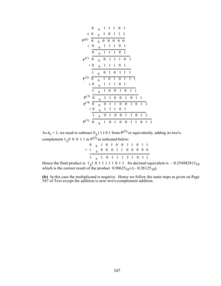
353. P(5)
+
+
P(2)
P(3)
P
(4)
1 ∆ 1 0 1 0 1
×
1 ∆ 1 0 1 0 1
0 ∆ 1 0 1 1 1
P(0)
P(1)
0 ∆ 0 0 0 0 0
1 ∆ 1 0 1 0 1
1 ∆ 1 0 1 0 1
1 ∆ 1 0 1 0 1
+
+
1 ∆ 1 1 0 1 0 1
1 1 ∆ 0 1 1 1 1 1
1
1 ∆ 1 0 0 0 0 1
1 ∆ 1 1 0 0 0 0 1
1 1 ∆ 0 1 1 0 1 0 1
1
1 ∆ 0 1 1 1 0 0 1
1 ∆ 1 0 1 1 1 0 0 1
1 ∆ 1 1 0 1 1 1 0 0 1
1 ∆ 1 0 1 0 1
1 1 ∆ 1 0 0 0 0 1 0 0 1
1
1 ∆ 1 0 0 0 1 1 0 0 1
1 ∆ 1 1 0 0 0 1 1 0 0 1
Hence the result of the product 1∆1 0 1 0 1× 0∆1 0 1 1 1 is given by 1∆1 1 0 0 0 1 1 0 0 1.
The decimal equivalent is (– 0.312510)× 0.7187510 = – 0.22460937510.
8.58 The transformation cosω = α + βcos ˆω is equivalent to
e
jω
+ e
– jω
2
= α + β
e
j ˆω
+ e
– j ˆω
2








, which
by analytic continuation can be expressed as
z + z
−1
2
= α + β
ˆz + ˆz
−1
2







 . Now, let H(z) be a
Type I linear-phase FIR transfer function of degree 2M. As indicated in Eq. (6.143), H(z) can
be expressed as H(z) = z
–M
a[n]
z + z
−1
2








n=0
M
∑
n
with a frequency response given by
H(e
jω
) = e
– jMω
a[n](cos
n =0
M
∑ ω)
n
, with
(
H(ω) = a[n](cos
n =0
M
∑ ω)
n
denoting the amplitude function
or the zero-phase frequency response. The amplitude function or the zero-phase frequency
response of the transformed filter obtained by applying the mapping cosω = α + βcos ˆω is
349

354. therefore given by
(
H( ˆω ) = a[n](α +β cos
n =0
M
∑ ˆω)
n
. Or equivalently, the transfer function of the
transformed filter is given by H(ˆz) = ˆz
–M
a[n] α + β
ˆz + ˆz
−1
2








n=0
M
∑
n
. A convenient way to realize
H(ˆz) is to consider the realization of the parent transfer function H(z) in the form of a Taylor
structure as outlined in Problem 6.23 which is obtained by expressing H(z) in the form
H(z) = a[n]z
–M+n 1+ z
−2
2








n=0
M
∑
n
. Similarly, the transfer function of the transformed filter can
be expressed as H(ˆz) = a[n]ˆz
–M+n
α ˆz
–1
+ β
1+ ˆz
−2
2








n=0
M
∑
n
. As a result, the transformed filter
can be realized by replacing each block
1+ z
−2
2
in the Taylor structure realization of H(z) by
the block α ˆz
–1
+β
1+ ˆz
−2
2
.
Now, for a lowpass-to-lowpass transformation, we can impose the condition
(
H( ˆω ) ˆω=0
=
(
H(ω)
ω=0
. This condition is met if α + β =1 and 0 ≤ α < 1. In this case, the
transformation reduces to cosω = α + (1−α)cos ˆω . From the plot of the mapping given below
it follows that as α is varied between 0 and 1, ˆω c < ωc .
cosω
cos ˆω
On the other hand if ˆω c > ωc is desired along with a lowpass-to-lowpass transformation, we can
impose the condition
(
H( ˆω ) ˆω=π
=
(
H(ω)
ω=π
. This condition is met if β = 1+ α and −1< α ≤ 0.
The corresponding transformation is now given by cosω = α + (1+α)cos ˆω . From the plot of
the mapping given below it follows that as α is varied between –1 and 0, ˆω c > ωc .
350

355. cosω
cos ˆω
M8.1 H(z) =
0.052817 + 0.079708z−1
+ 0.1295z−2
+ 0.1295z−3
+ 0.079708z−4
+ 0.052817z−5
1−1.8107 z−1 + 2.4947z−2 −1.8801z−3 + 0.95374z−4 − 0.23359z−5
0 10 20 30
-0.2
0
0.2
0.4
0.6
Time index n
M8.2 H(z) =
0.0083632− 0.033453z−1
+ 0.050179z−2
− 0.033453z−3
+ 0.0083632z−4
1+ 2.3741z−1 + 2.7057z−2 + 1.5917z−3 + 0.41032z−4
0 10 20 30
-0.4
-0.2
0
0.2
0.4
Time index n
M8.3 Numerator coefficients
Columns 1 through 7
2.7107e-04 0 -1.8975e-03 0 5.6924e-03 0 -9.4874e-03
351

356. Columns 8 through 14
0 9.4874e-03 0 -5.6924e-03 0 1.8975e-03 0
Column 15
-2.7107e-04
Denominator coefficients
Columns 1 through 5
1.0000e+00 1.7451e+00 4.9282e+00 6.1195e+00 9.8134e+00
Columns 6 through 10
9.2245e+00 1.0432e+01 7.5154e+00 6.4091e+00 3.4595e+00
Columns 11 through 15
2.2601e+00 8.4696e-01 4.1671e-01 8.5581e-02 2.9919e-02
0 10 20 30
-0.2
-0.1
0
0.1
0.2
0.3
Time index n
M8.4 Modified Program 8_2 is given below:
n = 0:60;
w = input('Angular frequency vector = ');
num = input('Numerator coefficients = ');
den = input('Denominator coefficients = ');
w = input('Normalized angular frequency vector = ');
x1 = cos(w(1)*pi*n); x2 = cos(w(2)*pi*n);
x = x1+x2;
subplot(2,1,1);
stem(n,x);
title('Input sequence');
xlabel('Time index n');ylabel('Amplitude');
[N,Wn] = ellipord(0.4,0.5,0.5,40);
[num,den] = ellip(N,0.5,40,Wn);
y = filter(num,den,x);
subplot(2,1,2);
stem(n,y);
title('Output sequence');
xlabel('Time index n'); ylabel('Amplitude');
The plots generated by this program for the filter of Example 7.19 for an input composed of
a sum of two sinusoidal sequences of angular frequencies, 0.3π and 0.6π, are given below:
352

357. 0 20 40 60
-2
-1
0
1
2
Input sequence
Time index n
0 20 40 60
-1
-0.5
0
0.5
1
Output sequence
Time index n
The blocking of the high-frequency signal by the lowpass filter can be demonstrated by
replacing the statement stem(k,x); with stem(k,x2); and the statement
y = filter(num,den,x)in the above program with the following:
y = filter(num,den,x2). The plots of the input high-frequency signal
component and the corresponding output are indicated below:
0 20 40 60
-1
-0.5
0
0.5
1
Input sequence
Time index n
0 20 40 60
-0.2
-0.1
0
0.1
0.2
0.3
Output sequence
Time index n
M8.5 The plots generated by using the modified program of Problem M8.4 and using the data of
this problem are shown below:
0 20 40 60
-2
-1
0
1
2
Input sequence
Time index n
0 20 40 60
-1
-0.5
0
0.5
1
1.5
Output sequence
Time index n
The blocking of the low-frequency signal by the highpass filter can be demonstrated by
replacing the statement stem(k,x); with stem(k,x1); and the statement
y = filter(num,den,x) in the above program with the following:
y = filter(num,den,x1). The plots of the input high-frequency signal
component and the corresponding output are indicated below:
353

358. 0 20 40 60
-1
-0.5
0
0.5
1
Input sequence
Time index n
0 20 40 60
-0.4
-0.2
0
0.2
0.4
Output sequence
Time index n
M8.6 % The factors for the transfer of example 7.16 are
% num1 = [0.2546 0.2546 0]
% den1 = [1.0000 -0.4909 0]
% num2 = [0.2982 0.1801 0.2982]
% den2 = [1.0000 -0.7624 0.5390]
% num3 = [0.6957 -0.0660 0.6957]
% den3 = [1.0000 -0.5574 0.8828]
N = input('The total number of sections = ');
for k = 1:N;
num(k,:) = input('The numerator = ');
den(k,:) = input('The denominator = ');
end
n = 0:60;
w = input('Normalized angular frequency vector = ');
x1 = cos(w(1)*pi*n); x2 = cos(w(2)*pi*n);
x = x1+x2;
subplot(2,1,1);
stem(n,x);
xlabel('Time index n'); ylabel('Amplitude');
title('Input sequence')
si = [0 0];
for k = 1:N
y(k,:) = filter(num(k,:),den(k,:),x,si);
x = y(k,:);
end
subplot(2,1,2);
stem(n,x);axis([0 50 -4 4]);
xlabel('Time index n'); ylabel('Amplitude');
title('Output sequence')
M8.7 %The factors for the highpass filter are
% num1 = [0.0495 -0.1006 0.0511]
% den1 = [1.0000 1.3101 0.5151]
% num2 = [0.1688 -0.3323 0.1636]
% den2 = [1.0000 1.0640 0.7966]
M8.8 To apply the function direct2 to filter a sum of two sinusoidal sequences, we replace the
statement y = filter(num,den,x,si) in the MATLAB program given in the
solution of Problem M8.4 with the statement y = direct2(num,den,x,si). The
plots generated by the modified program for the data given in this problem are given below:
354

359. M8.9 The MATLAB program that can be used to compute all DFT samples using the function gfft
and the function fft is as follows:
clear
N = input('Desired DFT length = ');
x = input('Input sequence = ');
for j = 1:N
Y(j) = gfft(x,N,j-1);
end
disp('DFT samples computed using gfft are ');
disp(Y);
disp('DFT samples computed using fft are ');
X = fft(x,N); disp(X);
Results obtained for the computation of two input sequences {x[n]} of lengths 8, and 12,
respectrively, are given below:
Desired DFT length = 8
Input sequence = [1 2 3 4 4 3 2 1]
FFT values computed using gfft are
Columns 1 through 4
20.0000 -5.8284 + 2.4142i 0 -0.1716 + 0.4142i
Columns 5 through 8
0 -0.1716 - 0.4142i 0 -5.8284 - 2.4142i
FFT values using fft are
Columns 1 through 4
20.0000 -5.8284 - 2.4142i 0 -0.1716 - 0.4142i
Columns 5 through 8
0 -0.1716 + 0.4142i 0 -5.8284 + 2.4142i
Desired DFT length = 12
Input sequence = [2 4 8 12 1 3 5 7 9 6 0 1]
FFT values computed using gfft are
Columns 1 through 4
58.0000 -8.3301 + 5.5000i -12.5000 +19.9186i
-1.0000 - 7.0000i
Columns 5 through 8
8.5000 - 7.7942i 0.3301 + 5.5000i -8.0000
0.3301 - 5.5000i
Columns 9 through 12
8.5000 + 7.7942i -1.0000 + 7.0000i -12.5000
355

360. -19.9186i -8.3301 - 5.5000i
FFT values using fft are
Columns 1 through 4
58.0000 -8.3301 - 5.5000i -12.5000 -19.9186i
-1.0000 + 7.0000i
Columns 5 through 8
8.5000 + 7.7942i 0.3301 - 5.5000i -8.0000 + 0.0000i
0.3301 + 5.5000i
Columns 9 through 12
8.5000 - 7.7942i -1.0000 - 7.0000i -12.5000
+19.9186i -8.3301 + 5.5000i
M8.10 The MATLAB program that can be used to verify the plots of Figure 8.37 is given below:
[z,p,k] = ellip(5,0.5,40,0.4);
a = conv([1 -p(1)],[1 -p(2)]);b =[1 -p(5)];
c = conv([1 -p(3)],[1 -p(4)]);
w = 0:pi/255:pi;
alpha = 0;
an1 = a(2) + (a(2)*a(2) - 2*(1 + a(3)))*alpha;
an2 = a(3) + (a(3) -1)*a(2)*alpha;
g = b(2) - (1 - b(2)*b(2))*alpha;
cn1 = c(2) + (c(2)*c(2) - 2*(1 + c(3)))*alpha;
cn2 = c(3) + (c(3) -1)*c(2)*alpha;
a = [1 an1 an2];b = [1 g]; c = [1 cn1 cn2];
h1 = freqz(fliplr(a),a,w); h2 = freqz(fliplr(b),b,w);
h3 = freqz(fliplr(c),c,w);
ha = 0.5*(h1.*h2 + h3);ma = 20*log10(abs(ha));
alpha = 0.1;
an1 = a(2) + (a(2)*a(2) - 2*(1 + a(3)))*alpha;
an2 = a(3) + (a(3) -1)*a(2)*alpha;
g = b(2) - (1 - b(2)*b(2))*alpha;
cn1 = c(2) + (c(2)*c(2) - 2*(1 + c(3)))*alpha;
cn2 = c(3) + (c(3) -1)*c(2)*alpha;
a = [1 an1 an2];b = [1 g]; c = [1 cn1 cn2];
h1 = freqz(fliplr(a),a,w); h2 = freqz(fliplr(b),b,w);
h3 = freqz(fliplr(c),c,w);
hb = 0.5*(h1.*h2 + h3);mb = 20*log10(abs(hb));
alpha = -0.25;
an1 = a(2) + (a(2)*a(2) - 2*(1 + a(3)))*alpha;
an2 = a(3) + (a(3) -1)*a(2)*alpha;
g = b(2) - (1 - b(2)*b(2))*alpha;
cn1 = c(2) + (c(2)*c(2) - 2*(1 + c(3)))*alpha;
cn2 = c(3) + (c(3) -1)*c(2)*alpha;
a = [1 an1 an2];b = [1 g]; c = [1 cn1 cn2];
h1 = freqz(fliplr(a),a,w); h2 = freqz(fliplr(b),b,w);
h3 = freqz(fliplr(c),c,w);
hc = 0.5*(h1.*h2 + h3);mc = 20*log10(abs(hc));
plot(w/pi,ma,'r-',w/pi,mb,'b--',w/pi,mc,'g-.');axis([0 1 -80
5]);
xlabel('Normalized frequency');ylabel('Gain, dB');
legend('b--','alpha = 0.1 ','w','','r-','alpha = 0
','w','','g-.','alpha = –0.25 ');
M8.11 The MATLAB program that can be used to verify the plots of Figure 8.39 is given below:
w = 0:pi/255:pi;
356

361. wc2 = 0.31*pi;
f = [0 0.36 0.46 1];m = [1 1 0 0];
b1 = remez(50, f, m);
h1 = freqz(b1,1,w);
m1 = 20*log10(abs(h1));
n = -25:-1;
c = b1(1:25)./sin(0.41*pi*n);
d = c.*sin(wc2*n);q = (b1(26)*wc2)/(0.4*pi);
b2 = [d q fliplr(d)];
h2 = freqz(b2,1,w);
m2 = 20*log10(abs(h2));
wc3 = 0.51*pi;
d = c.*sin(wc3*n);q = (b1(26)*wc3)/(0.4*pi);
b3 = [d q fliplr(d)];
h3 = freqz(b3,1,w);
m3 = 20*log10(abs(h3));
plot(w/pi,m1,'r-',w/pi,m2,'b--',w/pi,m3,'g-.');
axis([0 1 -80 5]);
xlabel('Normalized frequency');ylabel('Gain, dB');
legend('b--','wc = 0.31π','w','','r-','wc = 0.41π','w','','g-
.','wc = 0.51π')
M8.12 The MATLAB program to evaluate Eq. (8.104) is given below:
x = 0:0.001:0.5;
y = 3.140625*x + 0.0202636*x.^2 - 5.325196*x.^3 +
0.5446778*x.^4 + 1.800293*x.^5;
x1 = pi*x;
z = sin(x1);
plot(x,y);xlabel('Normalized angle,
radians');ylabel('Amplitude');
title('Approximate sine values');grid;axis([0 0.5 0 1]);
pause
plot(x,y-z);xlabel('Normalized angle,
radians');ylabel('Amplitude');
title('Error of approximation');grid;
The plots generated by the above program are as indicated below:
M8.13 The MATLAB program to evaluate Eq. (8.110) is given below:
k = 1;
357

362. for x = 0:.01:1
op1 = 0.318253*x+0.00331*x^2-0.130908*x^3+0.068524*x^4-
0.009159*x^5;
op2 = 0.999866*x-0.3302995*x^3+0.180141*x^5-
0.085133*x^7+0.0208351*x^9;
arctan1(k) = op1*180/pi;
arctan2(k) = 180*op2/pi;
actual(k) = atan(x)*180/pi;
k = k+1;
end
subplot(211)
x = 0:.01:1;
plot(x,arctan2);
ylabel('Angle, degrees');
xlabel('Tangent Values');
subplot(212)
plot(x,actual-arctan2,'--');
ylabel('Tangent Values');
xlabel('error, radians');
The plots generated by the above program are as indicated below:
Note: Expansion for arctan(x) given by Eq. (8.110) gives the result in normalized radians, i.e.
the actual value in radians divided by π.
358

363. Chapter 9 (2e)
9.1 Two's Complement Truncation - Assume x > 0. The relative error et is given by
et =
Q (x) − x
x
=
Q (M) − M
M
=
a−i 2−i
i=1
b
∑ − a−i 2−i
i =1
β
∑
M
=
− a−i 2−i
i=b+1
β
∑
M
.
Now et will be a minimum if all a-i's are 1 and will be a maximum if all a-i's are 0 for
b +1≤ i ≤ β , Thus –
δ
M
≤ et ≤
0
M
. Since 0.5 ≤ M ≤ 1 hence −2δ ≤ et ≤ 0.
Now consider x < 0. Here, the relative error et is given by
et =
Q (x) − x
x
=
Q (M) − M
M
=
−1+ a−i 2−i
i=1
b
∑ + 1− a−i 2−i
i =1
β
∑
M
. As before, –
δ
M
≤ et ≤
0
M
. In
this case –1 < M ≤ – 0.5, and, hence 0≤ et ≤ 2δ.
Ones' Complement Truncation - Assume again x > 0. The relative error et is given by
et =
Q (x) − x
x
=
Q (M) − M
M
=
a−i 2−i
i=1
b
∑ − a−i 2−i
i =1
β
∑
M
=
− a−i 2−i
i=b+1
β
∑
M
.
Now et will be a minimum if all a-i's are 1 and will be a maximum if all a-i's are 0 for
b +1≤ i ≤ β , Thus –
δ
M
≤ et ≤
0
M
. Since 0.5 ≤ M ≤ 1 hence −2δ ≤ et ≤ 0.
Now consider x < 0. Here, the relative error et is given by
et =
Q (x) − x
x
=
Q (M) − M
M
=
−(1− 2−b
) + a−i2−i
i=1
b
∑ + (1− 2−β
) − a−i 2−i
i=1
β
∑
M
=
(2−b
− 2−β
)+ a−i 2−i
i=b+1
b
∑
M
.
Now et will be a maximum if all a-i's are 0 and will be a minimum if all a-i's are 1, In this
case,
0
M
< et ≤
δ
M
. Since, – 0.5 ≤ M < – 1, hence –2δ < et ≤ 0.
Sign-Magnitude Truncation - Assume x > 0. Here,
et =
Q (M) − M
M
=
– a−i 2−i
i=1
b
∑ + a−i 2−i
i=1
β
∑
M
=
a−i 2−i
i=b+1
β
∑
M
. Since, – 1 ≤ M ≤ – 0.5, hence,
–2δ ≤ et < 0.
359

364. Rounding - ε = Q(M) – M. Hence
−δ
2
≤ ε ≤
δ
2
. This implies
−δ
2M
≤ er ≤
δ
2M
.
Since –1 < M ≤ – 0.5, and, hence − δ ≤ er ≤ δ.
9.2 The denominator is given by D(z) = z − α. Hence, the pole is at z = rejθ
= α where r = α and
θ = 0. The components of the pole sensitivities are therefore given by
∂r
∂α
=1 and
∂θ
∂α
= 0.
9.3 The denominator is given by D(z) = z2
− β(1+ α)z + α = (z − rejθ
)(z − r e−jθ
) = z2
− 2r cosθ + r2
.
Comparing we get, 2r cosθ = β(1+ α) and r2
= α. Hence, taking the partials of both sides of
the two equations we get
2r 0
2cosθ −2rsinθ




∆r
∆θ



 =
1 0
β 1+ α




∆α
∆β



 =
1 0
2rcosθ
1+r2
1+ r2








∆α
∆β



 or
∆r
∆θ



 =
2r 0
2cosθ −2r sinθ




−1 1 0
2rcosθ
1+r2
1+ r2








∆α
∆β



 =
1
2 r
0
(1−r2)cosθ
2 r2
(1+r2
)sin θ
−
1+r2
2 rsinθ












∆α
∆β



 .
The components of the pole sensitivities are therefore given by,
∂r
∂α
=
1
2r
,
∂r
∂β
= 0,
∂θ
∂α
=
(1− r2
)cotθ
2r2 (1+ r2)
, and
∂θ
∂β
= −
1+ r2
2rsinθ
.
9.4 Analysis of the digital filter structure yields
z
–1
z–1
c c
d d
–1
X(z) Y(z)
W(z) U(z) V(z)
W(z) = X(z) – Y(z),
U(z) = W(z) + cdz
−1
U(z) which implies U(z) =
W(z)
1− cdz−1 =
X(z) − Y(z)
1− c dz−1 ,
c z−1
V(z) = Y(z) implies V(z) =
zY(z)
c
. Also V(z) = c z−1
U(z) + dY(z).
Substituting for U(z) and V(z) we get
z Y(z)
c
= cz−1 X(z)− Y(z)
1− cdz−1 + dY(z). Thus,
Y(z){1 – c dz−1
– c dz−1
(1 – c dz−1
) + c2
z−2
} = c2
z−2
X(z), hence
H(z) =
Y(z)
X(z)
=
c2
z2 − 2c dz + c2 (1+ d2 )
.
Let c2(1 + d2) = r2 and c d = rcosθ, Solving we get cosθ =
d
1+ d2
.
Thus, d = cotθ and c = rsinθ. Hence, ∆d = − cosec2
θ(∆θ), and ∆c = sinθ(∆r)+ rcosθ(∆θ).
360

365. Or,
∆c
∆d



 =
sinθ r cosθ
0 −cosec2
θ




∆r
∆θ



 , i.e.
∆r
∆θ



 = −sin θ
− cosec2θ −r cosθ
0 sinθ






∆c
∆d



 =
1
sin θ
rsinθ⋅cosθ
0 − sin2
θ








∆c
∆d




z–1 z–1
c cd
– d
X(z) Y(z)
W(z)U(z) V(z)
Analysis of the above structure yields, U(z) = X(z) – dY(z)
V(z) = U(z) + c z−1
V(z) which implies V(z) =
U(z)
1− cz−1 .
W(z) = c dz−1
V(z) + c z−1
W(z) or W(z) =
cdz−1
1− cz−1 V(z) =
cdz−1
(1− cz−1)2 U(z) .
Y(z) = cz−1
W(z) or
Y(z)
cz−1 =
cdz−1 X(z) − dY(z)( )
(1− cz−1)2 .
Thus Y(z){(1 – c z−1
)2 + c2
dz−2
} = c2
dz−2
X(z). Hence,
H(z) =
Y(z)
X(z)
=
c2
d
z2 − 2cz + c2 (1+ d2 )
.
Again let c = rcosθ and c2(1 + d2) = r2.
Therefore, 1+ d2
= sec2
θ which implies d = tanθ. Taking partials we then get
∆ c = cosθ(∆ r)− rsinθ(∆θ), and ∆ d = sec2
θ(∆ θ). Thus,
∆c
∆d



 =
cosθ −rsinθ
0 sec2
θ




∆r
∆θ



 , which yields
∆r
∆θ



 =
1
cosθ
rsinθ⋅cosθ
0 cos2
θ








∆c
∆d



.
9.5
z–1 z–1
2
– b
–1
– c
X(z) Y(z)
S(z)
Analysis yields X(z) + 2z-1S(z) – b z-1S(z) – Y(z) – cY(z) = S(z) and Y(z) = z-2 S(z). Thus
H(z) =
Y(z)
X(z)
=
z−2
1+ (b− 2)z−1 + (1+ c)z−2 =
1
z2 + (b − 2)z + (1+ c)
.
361

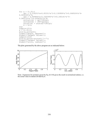
366. Let 1 + c = r2 and 2 − b = 2rcosθ. Taking partials we get
∆ c = 2r(∆ r), and –∆b = 2cosθ(∆ r) – 2rsinθ(∆θ). Equivalently,
∆c
∆b



 =
2r 0
2cosθ −2rsin θ




∆r
∆θ



 or
∆r
∆θ



 =
1
2r
0
1
2r2
tanθ
−
1
2rsinθ










∆c
∆b



 .
From Example 9.2 the pole sensitivities for Figure 9.9 are given by
∆r
∆θ



 =
cosθ sinθ
−
1
r
sinθ
1
r
cosθ








∆α
∆β



 .
9.6 (a) For direct form implementation B(z) = z3
+ b2z2
+ b1z + b0 = (z − z1)(z − z2 )(z − z3) where
z1 = r1ejθ1 , z2 = r1e– jθ1 , and z3 = r3ejθ3 . Thus, B(z) = (z2
− 2r1 cosθ1 z + r1
2
)(z − r3) =
(z2
+ 0.5111z + 0.7363)(z + 0.3628). Thus, 2r1 cosθ1 = −0.5111, r1
2
= 0.7363, r3 = 0.3628, and
θ3 = π.
From the above r1 = 0.7363 = 0.8581 and cosθ1 =
− 0.5111
2 0.7363
= −0.2978.
1
B(z)
=
1
(z2 + 0.5111z + 0.7363)(z + 0.3628)
=
− 0.7326 − j0.0959
z + 0.25555− j0.81914
+
−0.7326 + j0.0959
z + 0.25555 + j0.81914
+
1.4652
z + 0.3628
.
P1 = cosθ1 r1 r1
2
cosθ1[ ]= −0.2978 0.8581 −0.2193[ ],
Q1 = –sinθ1 0 r1
2
sin θ1[ ]= −0.9546 0 0.7029[ ],
R1 = 0.40357, X1 = – 0.36481,
P3 = cosθ3 r3 r3
2
cosθ1[ ]= −1 0.3628 − 0.1316[ ], Q3 = –sinθ3 0 r3
2
sinθ3[ ]= 0 0 0[ ],
R3 = 1.4652, and X3 = 0.
Thus, ∆r1 = –R1P1 + X1Q1( )⋅ ∆B = − 0.1266 ∆b0 + 0.6286∆b1 − 0.2281∆b2,
∆θ1 = –
1
r1
X1P1 + R1Q1( ) ⋅∆B = −0.8483 ∆b0 + 0.0959 ∆b1 + 0.5756 ∆b2 ,
∆r3 = –R3P3 + X3Q3( )⋅ ∆B = –R3P3 ⋅ ∆B = 1.4652∆b0 − 0.5316 ∆b1 + 0.1929 ∆b2 ,
∆θ3 = –
1
r3
X3P3 + R3Q3( )⋅ ∆B = 0.
(b) Cascade Form: B(z) = z3
+ b2z2
+ b1z + b0 = (z2
+ c1z + c0 )(z + d0) = B1(z)B2(z) where
B1(z) = z2
+ c1z + c0 = (z − z1)(z − z2 ) = (z − r1ejθ1 )(z − r1e–jθ1 ) = z2
− 2 r1 cosθ1z + r1
2
and
B2(z) = z + d0 = z − r3e jθ3. Comparing with the denominator of the given transfer function we
get 2r1 cosθ1 = −0.5111, r1
2
= 0.7363, r3 = 0.3628, and θ3 = π. Hence, r1 = 0.8581 and
cosθ1 = −0.2978.
Now,
1
B1(z)
=
−j 0.6104
z + 0.2556 − j0.8191
+
j 0.6104
z + 0.2556 + j0.8191
.
362

367. Hence, R1 = 0 and X1 = – 0.6104.
P1 = cosθ1 r1[ ]= −0.2978 0.8581[ ], and Q1 = –sinθ1 0[ ]= −0.9546 0[ ], Next, we observe
1
B2(z)
=
1
z + 0.3628
. This implies, R3 = 1 and X3 = 0. P3 = cosθ3 = −1, Q3 = −sinθ3 = 0.
Thus,
∆r1 = (−R1P1 + X1Q1) ⋅ ∆c0 ∆c1[ ]
T
= X1Q1 ⋅ ∆c0 ∆c1[ ]
T
= 0.5827∆c0 ,
∆θ1 = –
1
r1
X1P1 + R1Q1( ) ⋅ ∆c0 ∆c1[ ]
T
= −0.2118∆c0 + 0.6104∆c1
∆r3 = (−R3P3 + X3Q3)⋅ ∆d0 = −R3P3 ⋅∆d0 = − ∆d0
∆θ3 = –
1
r3
X3P3 + R3Q3( )⋅ ∆d0 = –
1
r3
R3Q3 ⋅∆d0 = 0
9.7 In terms of transfer parameters, the input-output relation of the two-pair of Figure P9.3 is given
by
Y1 = t11X1 + t12X2, and Y2 = t21X1 + t22X2, where X2 = αY2 . From Eq. (4.156b) we get
H(z) =
Y1(z)
X1(z)
= t11 +
α t12t21
1– α t22
.
From the above,
∂H(z)
∂α
=
t12t21 1–α t22( )+ t22α t12t21
1–α t22( )2 =
t12t21
1– αt22( )2 .
Substituting X2 = αY2 in Y2 = t21X1 + t22X2 we get the expression for the scaling transfer
function
Fα(z) =
Y2(z)
X1(z)
=
t21
1–α t22
. Now from the structure given below we observe that the noise
transfer function Gα(z) is given by Gα(z) =
Y1
U X1
=0
. From the structure we also observe that
X2 = αY2 + U. Substituting this in the transfer relations we arrive at with X1 = 0,
Y1 = t12X2 = t12(αY2 + U), and Y2 = t22X2 = t22(αY2 + U). From these two equations we
obtain
Y1
Y2
X1
α
U
X2
after some algebra Y1 =
α t12t22
1−α t22
U + t12U =
t12
1− αt22
U. Hence the noise transfer function is
given by Gα(z) =
Y1
U X1
=0
=
t12
1−α t22
. Therefore,
∂H(z)
∂α
=
t21
1– α t22
⋅
t12
1– αt22
= Fα(z)Gα(z).
363

368. 9.8 (a) WN (ω) =
1
2N +1
N +
sin (N + 1)ω[ ]
sin(ω)














1/ 2
=
1
2N + 1
1+ 4 cos2
(ωn)
n=1
N/ 2
∑














1/2
.
Since the maximum value of cos2
(ωn) = 1 and the minimum value = 0, hence
max{ WN (ω)} =
1
2N + 1
1+ 4 N / 2( )( )



1/2
= 1, and min{WN (ω)} =
1
2N + 1




1/2
> 0.
Hence 0 < WN (ω) ≤ 1.
(b) WN (0) =
1
2N +1
1+ 4 1
m=1
N /2
∑














1/ 2
= 1.
WN (π) =
1
2N + 1
1 + 4 1
m=1
N/ 2
∑














1/2
= 1.
(c) lim
N→∞
WN(π) = lim
N→∞
N
2N + 1
+ lim
N→∞
1
2N +1
sin((N + 1)ω)
sin(ω)






1/2
.
Since sin((N + 1)ω) ≤ 1 , lim
N→∞
1
2N + 1
sin((N+)ω)
sin(ω)
= 0, and lim
N→∞
WN(π) =
1
2
.
9.9 From Eq. (9.75) SNRA / D = 6.0206 b+16.81– 20 log10(K) dB. For a constant value of K, an
increase in b by 1 bit increases the SNRA/D by 6.0206 dB and an increase in b by 2 bits
increases the SNRA/D by 12.0412 dB.
If K = 4 and b = 7 then SNRA/D = 6.0206 × 7+16.81– 20 log10(4)
= 6.0206 × 7+16.81– 20 × 0.6021 = 46.9122 dB. Therefore for K = 4 and b = 9, SNRA/D =
46.91 + 12.04 = 58.95 dB; for K = 4 and b = 11, SNRA/D = 58.95 + 12.04 = 70.99 dB; for K
= 4 and b = 13, SNRA/D = 70.99+ 12.04 = 83.03; for K = 4 and b = 15, SNRA/D = 83.03 +
12.04 = 95.08.
If K = 6 and b = 7 then SNRA/D = 6.0206 × 7+16.81– 20 log10(6)
= 6.0206 × 7+16.81– 20 × 0.7782 = 43.3902 dB. Therefore for K = 6 and b = 9, SNRA/D =
43.39 + 12.04 = 55.43 dB; for K = 6 and b = 11, SNRA/D = 43.39 + 12.04 = 67.47 dB; for K
= 6 and b = 13, SNRA/D = 67.47 + 12.04 = 79.51; for K = 6 and b = 15, SNRA/D = 79.51 +
12.04 = 91.56.
If K = 8 and b = 7 then SNRA/D = 6.0206 × 7+16.81– 20 log10(8)
= 6.0206 × 7+16.81– 20 × 0.9031 = 40.8922 dB. Therefore for K = 6 and b = 9, SNRA/D =
40.89 + 12.04 = 52.93 dB; for K = 6 and b = 11, SNRA/D = 52.93 + 12.04 = 64.97 dB; for K
= 6 and b = 13, SNRA/D = 64.97 + 12.04 = 77.01; for K = 6 and b = 15, SNRA/D = 77.01 +
12.04 = 89.05.
9.10 (a) H(z) =
Ak
z + akk=1
N
∑ = Ck
akz +1
z + akk =1
N
∑ − Ckak
k =1
N
∑ = CkFk(z)
k =1
N
∑ + B, where Ck =
Ak
1− ak
2 ,
Fk (z) =
akz +1
z + ak
, and B = − Ck ak
k =1
N
∑ .
364

369. (b) σo
2
=
1
2πj
H(z)H(z−1
)z−1
dz
C
∫ =
1
2πj
CkFk(z)
k =1
N
∑ + B







 CkFk (z−1
)
k =1
N
∑ + B







 z−1
dz
C
∫
=
1
2πj
B2
C
∫ z−1
dz+ B Ck
k=1
N
∑ Fk (z)z−1
C
∫ dz + B Cl
l =1
N
∑ Fl (z−1
)z−1
C
∫ dz
+ CkCl
l =1
N
∑
k=1
N
∑
1
2πj
Fk(z)Fk(z−1
)z−1
C
∫ dz.
Now,
1
2πj
B2
z−1
C
∫ dz = B2
,
1
2πj
Fk(z)z−1
C
∫ dz = ak,
1
2πj
Fl (z)z−1
C
∫ dz = al , and
1
2πj
Fk(z)Fk(z−1
)z−1
C
∫ dz =
1− ak
2 − al
2 + akal
1− akal
. Therefore,
σo
2
= B2
+ 2 BCkak
k =1
N
∑ +
1− ak
2 − al
2 + akal
1− akall =1
N
∑
k=1
N
∑ . Since, Ckak
k=1
N
∑ = −B,
σo
2
= −B2
+
1− ak
2 − al
2 + akal
1− akall =1
N
∑
k=1
N
∑ CkCl
= − CkCl akal
l =1
N
∑
k=1
N
∑ + CkCl
1− ak
2 − al
2 + akal
1− akall =1
N
∑
k=1
N
∑
= CkCl
1− ak
2 − al
2 + akal
1− akal
− akal








l =1
N
∑
k =1
N
∑ =
Ak
(1− ak
2 )
⋅
Al
(1−al
2 )
1− ak
2 − al
2 + ak
2 al
2
1−akal








l =1
N
∑
k =1
N
∑
=
Ak
(1− ak
2 )
⋅
Al
(1−al
2 )
(1− ak
2 )(1− al
2)
1− akal








l =1
N
∑
k =1
N
∑ =
AkAl
1− akal
.
l =1
N
∑
k =1
N
∑ (A)
Further, σo
2
=
Ak
2
1− ak
2 +
AkAl
1− akall =k +1
N
∑
k=1
N−1
∑
k =1
N
∑ +
AkAl
1− akalk =l +1
N
∑
l =1
N−1
∑
=
Ak
2
1−ak
2 + 2
AkAl
1− akall =k+1
N
∑
k =1
N−1
∑
k =1
N
∑ .
(c) See Eq.(A).
9.11 (a) H1(z) =
(z + 3)(z −1)
(z − 0.5)(z + 0.3)
= 1+
− 2.1875
z − 0.5
+
4.3875
z + 0.3
. Making use of Eq. (9.86) and Table
9.4, we get σ1,n
2
= 1+
(−2.1875)2
1− (0.5)2 +
(4.3875)2
1− (0.3)2 +
2 × (−2.1875)× 4.3875
1− 0.15
= 1+ 6.3802 + 21.154 −16.692 =11.843.
Output of Program 9_4 is 11.843.
365

370. (b) H2(z) =
3(2z +1)(0.5z2
− 0.3z +1)
(3z +1)(4z +1)(z2 − 0.5z + 0.4)
=
−1.7049
z +
1
3
+
2.8245
z +
1
4
+
−0.86955z + 0.52675
z2 − 0.5z + 0.4
. Again,
from Eq. (9.86) and Table 9.44, we get σ2,n
2
=
(1.7049)2
1− 1
3( )
2 +
(2.8245)2
1− 1
4( )
2 + 2
−1.7049 × 2.8245
1−
1
12










+ 2 ×
−1.7049 −0.86955+ 0.52675× (−1/ 3)( )
1− 0.5(−1/ 3)+ 0.4(−1/3)2 + 2 ×
2.8245 −0.86955 + 0.52675× (−1/ 4)( )
1− 0.5(−1/ 4) + 0.4(−1/ 4)2
+
[(−0.86955)2
+ (0.52675)2
](1− 0.42
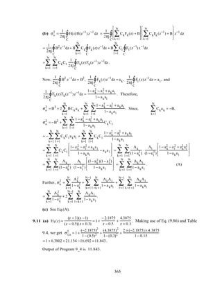
)− 2 × (−0.86955)× 0.52675× (1− 0.4) ×(−0.5)
(1− 0.42)2 + 2(0.4)(−0.5)2 −(1+ 0.42 )× (−0.5)2
= 3.271+ 8.5097 − 10.5065 + 2.9425 − 4.9183 + 0.9639 = 0.2613 .
Output of Program 9_4 is 0.26129.
(c) H3z) =
(z −1)2
z2 − 0.4z + 0.7
= 1+
−1.6z + 0.3
z2 − 0.4z + 0.7
. Again, from Eq. (9.86) and Table 9.44, we
get σ3,n
2
= 1+
(1.62
+ 0.32
)(1− 0.72
)− 2 × 0.3× (−1.6)× (−0.4)× (1− 0.7)
(1− 0.72 )+ 2 × 0.7× 0.42 − (1+ 0.72) × 0.42 = 1 + 5.0317 = 6.0317.
Output of Program 9_4 is 6.0317.
9.12 H(z) = C +
A
1− αz−1 +
B
1−β z−1 = C +
Az
z − α
+
Bz
z − β
= C +
Az − Aα + Aα
z − α
+
Bz − Bβ + Bβ
z − β
= (A + B + C) +
Aα
z − α
+
Bβ
z − β
. From Eq. (9.86) and using Table 9.4 we obtain
σv,n
2
= (A + B+ C)2
+
(Aα)2
1− α2 +
(Bβ)2
1− β2 +
2AαBβ
1− αβ
. For the values given, we get
σv,n
2
= (3)2
+
(0.7 × 3)2
1− (0.7)2 +
(2× 0.9)2
1− (0.9)2 +
2× 3× (−0.7) × (−2) × 0.9
1− (−0.7)(0.9)
= 16 + 8.6471+ 17.053 + 4.638 = 46.338
Output of Program 9_4 is 4.6338.
9.13 (a) Quantization of products before addition.
Cascade Structure #1: H(z) =
1− 2z−1
1+ 0.3z−1






1+ 3z−1
1− 0.4z−1





 . The noise model of this structure is
shown below:
−2
z
−1
z
−1
− 0.3 0.4
3
e1[n]
e2[n]
e3[n]
e4[n]
366

371. The noise transfer function from the noise source e1[n] to the filter output is
G1(z) = H(z) =
z2
+ z − 6
z2 − 0.1z − 0.12
= 1+
−7.7714
z − 0.4
+
8.8714
z + 0.3
. The corresponding normalized noise
variance at the output is σ1
2
=1+
(−7.7714)2
1− (0.4)2 +
(8.8714)2
1−(−0.3)2 + 2
−7.7714 × 8.8714
1− (0.4)(−0.3)





 = 36.271.
The noise transfer function from the noise sources e2[n] and e3[n] to the filter output is
G2(z) =
z + 3
z − 0.4
= 1+
3.4
z − 0.4
. The normalized noise variance at the output due to each of these
noise sources is σ2
2
=1+
(3.4)2
1− (0.4)2 = 14.762. The noise transfer function from the noise source
e4[n] to the filter output is G3(z) = 1, The corresponding normalized noise variance at the
output is σ3
2
=1. Hence the total noise variance at the output is σo
2
= σ1
2
+ 2σ2
2
+ σ3
2
= 66.795.
Cascade Structure #2: H(z) =
1+ 3z−1
1+ 0.3z−1






1− 2z−1
1− 0.4z−1





 . The noise model of this structure is
shown below:
z
−1
z
−1
− 0.3 0.4
e1[n]
e2[n]
e3[n]
e4[n]
−23
The noise transfer function from the noise source e1[n] to the filter output is
G1(z) = H(z) =
z2
+ z − 6
z2 − 0.1z − 0.12
= 1+
−7.7714
z − 0.4
+
8.8714
z + 0.3
. The corresponding normalized noise
variance at the output is σ1
2
=1+
(−7.7714)2
1− (0.4)2 +
(8.8714)2
1−(−0.3)2 + 2
−7.7714 × 8.8714
1− (0.4)(−0.3)





 = 36.271.
The noise transfer function from the noise sources e2[n] and e3[n] to the filter output is
G2(z) =
z − 2
z − 0.4
= 1+
−1.6
z − 0.4
. The normalized noise variance at the output due to each of these
noise sources is σ2
2
=1+
(−1.6)2
1− (0.4)2 = 4.0476. The noise transfer function from the noise source
e4[n] to the filter output is G3(z) = 1, The corresponding normalized noise variance at the
output is σ3
2
=1. Hence the total noise variance at the output is σo
2
= σ1
2
+ 2σ2
2
+ σ3
2
= 45.366.
Cascade Structure #3: H(z) =
1+ 3z−1
1− 0.4z−1






1− 2z−1
1+ 0.3z−1





 . The noise model of this structure is
shown below:
367

372. z
−1
z
−1
e1[n]
e2[n]
e3[n]
e4[n]
−23
− 0.30.4
The noise transfer function from the noise source e1[n] to the filter output is
G1(z) = H(z) =
z2
+ z − 6
z2 − 0.1z − 0.12
= 1+
−7.7714
z − 0.4
+
8.8714
z + 0.3
. The corresponding normalized noise
variance at the output is σ1
2
=1+
(−7.7714)2
1− (0.4)2 +
(8.8714)2
1−(−0.3)2 + 2
−7.7714 × 8.8714
1− (0.4)(−0.3)





 = 36.271.
The noise transfer function from the noise sources e2[n] and e3[n] to the filter output is
G2(z) =
z − 2
z + 0.3
=1+
−2.3
z + 0.3
. The normalized noise variance at the output due to each of these
noise sources is σ2
2
=1+
(−2.3)2
1− (−0.3)2 = 6.8132. The noise transfer function from the noise source
e4[n] to the filter output is G3(z) = 1, The corresponding normalized noise variance at the
output is σ3
2
=1. Hence the total noise variance at the output is σo
2
= σ1
2
+ 2σ2
2
+ σ3
2
= 50.897.
Cascade Structure #4: H(z) =
1− 2z−1
1− 0.4z−1






1+ 3z−1
1+ 0.3z−1





 . The noise model of this structure is
shown below:
z
−1
z
−1
e1[n]
e2[n]
e3[n]
e4[n]
− 0.30.4
3−2
The noise transfer function from the noise source e1[n] to the filter output is
G1(z) = H(z) =
z2
+ z − 6
z2 − 0.1z − 0.12
= 1+
−7.7714
z − 0.4
+
8.8714
z + 0.3
. The corresponding normalized noise
variance at the output is σ1
2
=1+
(−7.7714)2
1− (0.4)2 +
(8.8714)2
1−(−0.3)2 + 2
−7.7714 × 8.8714
1− (0.4)(−0.3)





 = 36.271.
The noise transfer function from the noise sources e2[n] and e3[n] to the filter output is
G2(z) =
z + 3
z + 0.3
=1+
2.7
z + 0.3
. The normalized noise variance at the output due to each of these
noise sources is σ2
2
=1+
(2.7)2
1− (−0.3)2 = 9.011. The noise transfer function from the noise source
e4[n] to the filter output is G3(z) = 1, The corresponding normalized noise variance at the
output is σ3
2
=1. Hence the total noise variance at the output is σo
2
= σ1
2
+ 2σ2
2
+ σ3
2
= 55.293.
368

373. Hence, the Cascade Structure #2 has the smallest roundoffnoise variance.
(b) Quantization of products after addition.
From the results of Part (a) we have here the following roundoff noise varainces:
Cascade Structure #1: σo
2
= σ1
2
+ σ2
2
+ σ3
2
= 52.033.
Cascade Structure #2: σo
2
= σ1
2
+ σ2
2
+ σ3
2
= 41.319.
Cascade Structure #3: σo
2
= σ1
2
+ σ2
2
+ σ3
2
= 44.084.
Cascade Structure #4: σo
2
= σ1
2
+ σ2
2
+ σ3
2
= 46.282.
In this case also the Cascade Form 2 has the smallest roundoffnoise variance.
9.14 (a) Quantization of products before addition.
Parallel Form I: H(z) =
(z − 2)(z + 3)
(z + 0.3)(z − 0.2)
= 50 +
−19.429
1− 0.4z−1 +
−29.571
1+ 0.3z−1 . The noise model is as
shown below
z
−1
z
−1
e1[n ]
e2[n]
e3[n ]
e4[n] − 0.3
0.4
50
−19.429
29.571
e5[n]
–
The noise transfer function from the noise source e1[n] to the filter output is G1(z) = 1 and its
corresponding normalized noise variance at the output is σ1
2
=1. The noise transfer function
from the noise sources e2[n] and e3[n] to the filter output is
G2(z) =
1
1− 0.4z−1 =
z
z − 0.4
=1+
0.4
z − 0.4
. The normalized noise variance at the output due to
each of these noise sources is σ2
2
=1+
(0.4)2
1− (0.4)2 = 1.1905. The noise transfer function from the
noise sources e4[n] and e5[n] to the filter output is G3(z) =
1
1+ 0.3z−1 =
z
z + 0.3
= 1+
−0.3
z + 0.3
.
The normalized noise variance at the output due to each of these noise sources is
369

374. σ3
2
=1+
(−0.3)2
1− (−0.3)2 = 1.0989. Hence the total noise variance at the output is
σo
2
= σ1
2
+ 2σ2
2
+ 2σ3
2
= 5.5788.
Parallel Form II: H(z) = 1+
−7.7714
z − 0.4
+
8.8714
z + 0.3
= 1+
−7.7714 z−1
1− 0.4z−1 +
8.8714 z−1
1+ 0.3z−1 . The noise model
is as shown below
z
−1
z
−1
e2[n]
e3[n]
e4[n] − 0.3
0.4
e5[n]
8.8714
− 7.7714
The noise transfer function from the noise sources e2[n] and e3[n] to the filter output is
G2(z) =
z−1
1− 0.4z−1 =
1
z − 0.4
. The normalized noise variance at the output due to each of these
noise sources is σ2
2
=
1
1− (0.4)2 = 1.1905. The noise transfer function from the noise sources
e4[n] and e5[n] to the filter output is G3(z) =
z−1
1+ 0.3z−1 =
1
z + 0.3
. The normalized noise
variance at the output due to each of these noise sources is σ3
2
=
1
1− (−0.3)2 = 1.0989. Hence
the total noise variance at the output is σo
2
= 2σ2
2
+ 2σ3
2
= 4.5788.
Hence, Parallel Form #2 has the smaller roundoff noise variance.
(b) Quantization of products after addition.
Parallel Form I: From the results of Part (a) we note that the total noise variance at the output
is σo
2
= σ1
2
+ σ2
2
+ σ3
2
= 3.2894.
Parallel Form II: From the results of Part (a) we note that the total noise variance at the output
is σo
2
= σ2
2
+ σ3
2
= 2.2894.
9.15 H(z) =
2 + 2z−1
− 1.5z−2
1+ 0.5z−1
+ 0.06z−2 .
(a) The noise model of the Direct Form II realization of H(z) is shown below:
370

375. z
−1
z
−1e1[n]
e2[n]
e3[n]
e4[n]
e5[n]
2
2
−1,5
− 0.5
− 0.06
The noise transfer function from the noise sources e3[n], e4[n] and e5[n] to the filter output is
G2(z) = 1, and the noise transfer function from the noise sources e1[n] and e2[n] to the filter
output is G1(z) = H(z) =
2+ 2z−1
−1.5z−2
1+ 0.5z−1 − 0.06z−2 = 2 +
−18.2
z + 0.2
+
19.2
z + 0.3
. Using Table 9.4, the
normalized noise variance at the output due to each of the noise sources e1[n] and e2[n] is then
σ1
2
= 2 4+
(−18.2)2
1− (−0.2)2 +
(19.2)2
1− (−0.3)2 + 2
−18.2×19.2
1− (−0.2)(−0.3)














= 10.651,
and the normalized noise variance at the output due to each of the noise sources e3[n], e4[n]
and e5[n] is σ2
2
=1. Hence the total noise variance at the output is σo
2
= 2σ1
2
+ 3σ2
2
= 24.302.
(b) Cascade Form Realization: H(z) =
2(1− 0.5z−1
)(1+1.5z−1
)
(1+ 0.2z−1)(1+ 0.3z−1)
. There are more than 2
possible cascade realizations. We consider here only two such structures.
Cascade Form #1: H(z) = 2
1− 0.5z−1
1+ 0.2z−1






1+1.5z−1
1+ 0.3z−1





 . The noise model of this realization is
shown below:
z− 1
z− 1
−0,5 1.5−0.2 −0.3
2
e1[n]
e2 [n] e3[n] e4[n] e5[n]
The noise transfer function from the noise sources e1[n] and e2[n] to the filter output is
G1(z) =
1+1z−1
− 0.75z−2
1+ 0.5z−1 − 0.06z−2 =1+
−9.1
z + 0.2
+
9.6
z + 0.3
. Its contribution to the output noise variance
is σ1
2
=1+
(−9.1)(−9.1)
1− (−0.2)(−0.2)
+
(9.6)(9.6)
1− (−0.3)(−0.3)
+ 2
(−9.1)(9.6)
1− (−0.2)(−0.3)





 = 2.6628.
371

376. The noise transfer function from the noise sourcese3[n], and e4[n] to the filter output is
G2(z) =
1+1.5z−1
1+ 0.3z−1 = 1+
1.2
z + 0.3
. Its contribution to the output noise variance is
σ2
2
=1+
(1.2)2
1− (−0.3)2 = 2.5824. Finally, the noise transfer function from the noise source e5[n]
to the filter output is G3(z) = 1. Its contribution to the output noise variance is σ3
2
=1. Hence
the total noise variance at the output is σo
2
= 2σ1
2
+ 2σ2
2
+ σ3
2
= 2(2.6628)+ 2(2.5824)+1= 11.49.
Cascade Form #2: H(z) = 2
1+1.5z−1
1+ 0.2z−1






1− 0.5z−1
1+ 0.3z−1





 . The noise model of this realization is
shown below:
z−1
z−1
− 0.2 − 0.3
e1[n]
e2[n] e3[n] e4[n] e5[n]
1.5 − 0,5
2
The noise transfer function from the noise sources e1[n] and e2[n] to the filter output is
G1(z) =
1+1z−1
− 0.75z−2
1+ 0.5z−1 − 0.06z−2 =1+
−9.1
z + 0.2
+
9.6
z + 0.3
. Its contribution to the output noise variance
is σ1
2
=1+
(−9.1)(−9.1)
1− (−0.2)(−0.2)
+
(9.6)(9.6)
1− (−0.3)(−0.3)
+ 2
(−9.1)(9.6)
1− (−0.2)(−0.3)





 = 2.6628.
The noise transfer function from the noise sources e3[n], and e4[n] to the filter output is
G2(z) =
1− 0.5z−1
1+ 0.3z−1 = 1+
−0.8
z + 0.3
. Its contribution to the output noise variance is
σ2
2
=1+
(−0.8)2
1− (−0.3)2 = 1.7033, Finally, the noise transfer function from the noise source e5[n]
to the filter output is G3(z) = 1. Its contribution to the output noise variance is σ3
2
=1. Hence
the total noise variance at the output is σo
2
= 2σ1
2
+ 2σ2
2
+ σ3
2
= 2(2.6628)+ 2(1.7033) +1= 9.7322.
(c) Parallel Form I Realization: H(z) = −25+
91
1+ 0.2z−1 +
−64
1+ 0.3z−1 . The noise model of this
realization is shown below:
372

377. e5[n]
e4[n]
e3[n]
e2[n]
e1[n]
91
−0.2
−0.3
z−1
z−1
− 25
The noise transfer function from the noise sources e1[n] and e2[n] to the filter output is
G1(z) =
1
1+ 0.2z−1 =1 +
−0.2
z + 0.2
. Its contribution to the output noise variance is
σ1
2
=1+
(−0.2)2
1− (−0.2)2 = 1.0417.
The noise transfer function from the noise sources e3[n] and e4[n] to the filter output is
G2(z) =
1
1+ 0.3z−1 =1+
− 0.3
z + 0.3
. Its contribution to the output noise variance is
σ2
2
=1+
(−0.3)2
1− (−0.3)2 = 1.0989.
Finally, the noise transfer function from he noise sources e5[n] to the filter output is G3(z) = 1.
Its contribution to the output noise variance is σ3
2
=1. Hence the total noise variance at the
output is σo
2
= 2σ1
2
+ 2σ2
2
+ σ3
2
= 5.2812.
Parallel Form II Realization: H(z) = 2+
−18.2
z + 0.2
+
19.2
z + 0.3
. The noise model of this realization is
shown below:
z
−1
z
−1
− 0.2
− 0.3
e1[n]
e2[n]
e3[n]
e4[n]
2
19.2
−18.2 e5[n]
373

378. The noise transfer function from the noise sources e1[n] and e2[n] to the filter output is
G1(z) =
z−1
1+ 0.2z−1 =
1
z + 0.2
. Its contribution to the output noise variance is
σ1
2
=
1
1− (−0.2)2 = 1.0417.
The noise transfer function from the noise sources e3[n] and e4[n] to the filter output is
G2(z) =
z−1
1+ 0.3z−1 =
1
z + 0.3
. Its contribution to the output noise variance is
σ2
2
=
1
1− (−0.3)2 = 1.0989.
Finally, the noise transfer function from he noise sources e5[n] to the filter output is G3(z) = 1.
Its contribution to the output noise variance is σ3
2
=1. Hence the total noise variance at the
output is σo
2
= 2σ1
2
+ 2σ2
2
+ σ3
2
= 5.2812.
As a result, both Parallel Form structures have the smallest product roundoff noise variance.
9.16 H(z) =
2 + 2z−1
−1.5z−2
1+ 0.5z−1 − 0.06z−2 . Using Program 6_4, the Gray-Markel realization of H(z) is found
to be as shown below where d2 = 0.472, d1' = 0.06, α1 = −1.5, α2 = 2.75, and α3 = 0.793.
X1
Yo
–d2
d2
–d1'
d1'
z–1
z
–1
α1 α2
α3
Y1
S2 S1
W2
(a) For quantization of products before addition, the noise model is as shown below:
–d 2
d 2
–d1'
d1'
z–1
z–1
α1 α2
α3
x1[n]
y1[n]
yo[n] + γ[ n]
e1[n] e2[n]
e3[n]e4[n]
e5[n] e6[ n] e7[ n]
s1[n]s2[n]
Analyzing the above structure we obtain the noise transfer functions for each noise source,
ei[n], 1≤ i ≤ 7:
374

379. G1(z) = H(z) =
2+ 2z−1
−1.5z−2
1+ 0.5z−1 − 0.06z−2 ,
G2(z) =
(α2d1' +α3) + α1(1− d2
2
)d1' +α2[ ]z–1
+ α1(1− d2
2
)z–2
1+ 0.5z–1 + 0.06z–2 =
2.091+ 2.0445z–1
−1.495z–2
1+ 0.5z–1 + 0.06 z–2 ,
G3(z) =
α2 + α1(1− d2
2
)− α2d1' d2 − α3d2[ ]z–1
+ α1(1− d2
2
)d2d1' z–2
1+ 0.5z–1 + 0.06z–2 =
2.75 −1.6201z–1
− 0.7055 z–2
1+ 0.5z–1 + 0.06z–2 ,
G4(z) = α1 = −1.5,
G5(z) = G6(z) = G7(z) =1.
Using Program 9_4 we get σ1,n
2
= 10.651, σ2,n
2
= 11.021, σ3,n
2
= 16.945, σ4,n
2
= 2.25. Hence, the
total normalized output noise variances = 10.651 + 11.021 + 16.945 + 2.25 + 3(1) = 43.87.
(b) The noise model of the above structure assuming quntization of products after addition is
as given below:
x[n]
z
−1
z
−1
y[n]
− d2
d2
− d1
'
d1
'
α1 α2 α3
e2[n]
e5[n]
e4[n] e3[n]
The pertinent noise transfer functions here are: G2(z) =
2.091+ 2.0445z–1
−1.495z–2
1+ 0.5z–1 + 0.06z–2 ,
G3(z) =
2.75 −1.6201z–1
− 0.7055z–2
1+ 0.5z–1 + 0.06z–2 , G4(z) = −1.5, and G5(z) =1. Hence, the total
normalized output noise variances = 11.021 + 16.945 + 2.25 + 1 = 31.22.
9.17 The noise model of Figure P9.8 is as shown below:
z
−1
z
−1x[n] y[n]
−1 d1
d2
e1[n]
e2[n]
The noise transfer function from the noise sources e1[n] and e2[n] to the output is given by
375

380. G1(z) =
1− z−2
1+ d1
z−1 + d2
z−2 =
z2
−1
z2 + d1
z + d2
=1−
d1z + (1+ d2)
z2 + d1
z + d2
Using Table 9.4 we arrive at the total normalized output noise power as
σn
2
= 2 1+
d1
2
+ (1+ d2)2
( )(1− d2
2
) − 2 d1(1+ d2 )− d1(1+ d2 )d2( )d1
(1− d2
2)2 + 2d2
d1
2 − (1+ d2
2 )d1
2










= 2 1+
(1− d2
2
) (1+ d2)2
− d1
2
( )
(1− d2
)2 (1+ d2
)2 − d1
2
( )










=
4
1− d2
.
9.18 (a) Quantization of products before addition
The noise model second-order coupled form structure is shown below.
V(z)
U(z)
Y(z)
E1(z)
E2( z)
E3(z)
E4 (z)
z−1
z−1
α
β
γ
δ
We observe from Example 9.2 that α = δ = r cosθ , β = −γ = rsinθ, α + δ = 2rcosθ and
αδ − βγ = r2
.
Analysis yields U(z) = β z−1
Y(z) + αV(z)+ E3(z), V(z) = z−1
U(z), and
Y(z) = γ V(z) + δz−1
Y(z) + E1(z). Eliminating the variables U(z) and V(z) from these equations
we arrive at
1− (α + δ)z−1
+ (α δ −β γ)z−2
1− αz−1 Y(z) =
γ z−1
1− αz−1 E3(z) + E1(z). Hence, the noise
transfer function from the noise sources e1[n] and e2[n] to the output is given by
G1(z) =
Y(z)
E1(z) E3(z)=E4(z)=0
=
1− α z−1
1− (α + δ)z−1
+ (α δ − β γ)z−2 =
z2
− α z
z2
− (α + δ)z + (αδ − βγ)
= 1+
δz − (αδ −β γ)
z2 − (α + δ)z +(αδ − βγ)
= 1+
rcosθz − r2
z2 − 2rcosθz + r2 , and the noise transfer function from the
noise sources e3[n] and e4[n] to the output is given by
G2(z) =
Y(z)
E3 (z) E1(z)=E2(z)=0
=
γ z−1
1− (α + δ)z−1
+ (αδ − βγ)z−2 =
γ z
z2
− (α + δ)z + (α δ − β γ)
=
−rsinθ z
z2
− 2r cosθ z + r2 .
376

381. The output roundoff noise variance due to each of the noise sources e1[n] and e2[n] is
σ1
2
=1+
(r2
cos2
θ + r4
)(1− r4
)− 2(−r3
cosθ + r3
cosθ⋅r2
)(−2rcosθ)
(1− r4 )2 + 2r2(4r2 cos2 θ) −(1+ r4)(4r2 cos2 θ)
= 1+
r2
(1+ r2
)(r2
+ cos2
θ) − 4r4
cos2
θ
(1− r2 ) (1+ r2 )2 − 4r2 cos2 θ[ ]
, and the output roundoff noise variance due to each of
the noise sources e3[n] and e4[n] is σ2
2
=
r2
(1+ r2
)sin2
θ
(1− r2 ) (1+ r2 )2 − 4r2 cos2 θ[ ]
. Hence, the total
roundoff noise variance at the output is
σo
2
= 2(σ1
2
+ σ2
2
) = 2 1+
r2
(1+ r2
)(r2
+ cos2
θ)− 4 r4
cos2
θ
(1− r2) (1+ r2 )2 − 4r2 cos2 θ[ ]
+
r2
(1+ r2
)sin2
θ
(1− r2) (1+ r2 )2 − 4 r2 cos2 θ[ ]








.
(b) Quantization of products after addition
Here, the total roundoff noise variance at the output is
σo
2
= σ1
2
+ σ2
2
= 1+
r2
(1+ r2
)(r2
+ cos2
θ) − 4r4
cos2
θ
(1− r2 ) (1+ r2 )2 − 4r2 cos2 θ[ ]
+
r2
(1+ r2
)sin2
θ
(1− r2 ) (1+ r2 )2 − 4r2 cos2 θ[ ]
.
9.19 (a) Quantization of products before addition
The noise model of the Kingsbury structure is shown below:
x[n]
u[n] v[n]
y[n]
e1[n] e2[n]
e3[n]
− k1
k1 k2z
−1
z
−1
Analysis yields U(z) = k1Y(z) + E1(z), V(z) =
1
1− z−1 U(z)+ k2Y(z)+ E2(z), and
Y(z) = −k1V(z) + E3(z)[ ]
z−1
1− z−1 = −
k1z−1
1− z−1 V(z) +
z−1
1 − z−1 E3(z). Eliminating U(z) and V(z)
from these equations we arrive at
1 − 2 − k1(k1 + k2 )[ ]z−1
+ (1− k1k2)z−2
(1− z−1
)2 Y(z) = −
k1z−1
(1− z−1
)2 E1(z) −
k1z−1
1− z−1 E2(z) +
z−1
1− z−1 E3(z).
Hence, the noise transfer function from the noise source e1[n] to the output is given by
G1(z) =
Y(z)
E1(z) E2 (z)=E3(z)=0
=
− k1z−1
1− 2 − k1(k1 + k2 )[ ]z−1
+ (1− k1k2 )z−2 =
− k1z
z2
− 2r cosθ z + r2 . Its
corresponding output noise variance is thus given by
377

382. σ1
2
=
k1
2
(1− r4
)
(1− r4
)2
+ 2r2
(−2r cosθ)2
− (1+ r4
)(−2r cosθ)2 =
k1
2
(1− r2
)(1+ r2
)
(1− r2
)2
(1 + r2
)2
− 4 r2
cos2
θ(1 − r2
)2
=
k1
2
(1+ r2
)
(1− r2
) (1+ r2
)2
− 4r2
cos2
θ[ ]
.
The noise transfer function from the noise source e2[n] to the output is given by
G2(z) =
Y(z)
E2(z) E1(z)=E3(z)=0
=
− k1z−1
(1− z−1
)
1− 2 − k1(k1 + k2 )[ ]z−1
+ (1 − k1k2 )z−2 =
− k1z + k
z2
− 2rcosθz + r2 .
Its corresponding output noise variance is thus given by σ2
2
=
2k1
2
(1+ r2
)
(1− r2
) (1+ r2
)2
− 4r2
cos2
θ[ ]
.
Finally, the noise transfer function from the noise source e3[n] to the output is given by
G3(z) =
Y(z)
E3(z) E1(z)=E2(z)=0
=
z−1
(1− z−1
)
1− 2 − k1(k1 + k2 )[ ]z−1
+ (1− k1k2 )z−2 =
z −1
z2
− 2r cosθz + r2 Its
corresponding output noise variance is thus given by σ3
2
=
2(1+ r2
)
(1− r2
) (1+ r2
)2
− 4r2
cos2
θ[ ]
.
Hence, the total normalized output noise variance due to product roundoff before (after)
summation is given by σo
2
= σ1
2
+ σ2
2
+ σ3
2
=
3k1
2
+ 2( )(1+ r2
)
(1− r2
) (1+ r2
)2
− 4r2
cos2
θ[ ]
.
9.20 Let e[n] be a noise source due to product roundoff inside H(z) with an associated noise
transfer function Ge(z) to the output of H(z). Then the normalized noise power at the output
of the cascade structrure due to e[n] is given by σe,n
2
=
1
2πj
Ge(z)A2(z)Ge(z−1
)A2 (z−1
)
C
∫ z−1
dz
=
1
2πj
Ge(z)Ge(z−1
)
C
∫ z−1
dz since A2(z)A2 (z−1
) =1.
Assuming H(z) is realized in a cascade form with the lowest product roundoff noise power
σh,n
2
, the normalized noise power at the output of the cascade due to product roundoff in
H(z) still remains σh,n
2
. From the solution of Problem 9.13, we note that the lowest
roundoff noise power is σh,n
2
= 45.366 for cascade form #2. Next, from the solution of
Problem 9.17 we note that the normalized output noise power due to noise sources in A2(z) is
σa,n
2
=
4
1− d2
. Substituting d2 = 0.8 we get σa,n
2
=
4
1− 0.8
= 20. Hence total output noise
variance of the cascade is given by σo
2
= σh,n
2
+ σa,n
2
= 45.366+ 20 = 65.366.
9.21 The noise model for the structure is as shown below
378

383. z −1
z −1
0.4 − 0.5
e1[n] e2[n]
The noise transfer function from e1[n] to the output is
G1(z) =
1
(1− 0.4z−1)(1+ 0.5z−1)
= 1+
−27.778
z + 0.5
+
17.778
z − 0.4
. Thus, the normalized noise power at the
output due to e1[n] is σ1
2
=1+
−0.27778( )2
1− (−0.5)2 +
0.17778( )2
1− (0.4)2 + 2 ×
–0.27778( )× 0.17778( )
1−(−0.5)(0.4)
= 1.0582.
The noise transfer function from e2[n] to the output is G2(z) =
1
1+ 0.5z−1 = 1+
−0.5
z + 0.5
.
Thus, the normalized noise power at the output due to e2[n] is σ2
2
=1+
−0.5( )2
1− −0.5( )2 = 1.3333.
Therefore, the total normalized noise at the output = 1.0582 + 1.3333 = 2.3915.
For a 9-bit signed two's-complement number representation, the quantization level
δ = 2−8
= 0.0039062. Hence, the total output noise power due to product roundoff is
σo
2
=
δ2
12
(2.3915) = 3.0409 ×10−6
.
9.22 The unscaled structure is shown below.
z−1
0.5 −0.3
F1 (z)
X(z) Y(z)
Now, F1(z) =
1
1− 0.5z−1 =1+
0.5
z − 0.5
. Using Table 9.4 we obtain F1 2
2
= 1+
(0.5)2
1− (0.5)2 = 1.3333.
Next, H(z) =
1− 0.3z−1
1− 0.5z−1 =
z − 0.3
z – 0.5
=1+
0.2
z –0.5
. Using Table 9.4 we obtain
H 2
2
= 1+
(0.2)2
1− (0.5)2 = 1.0533.
From Eq. (9.129a), F1 2
= α1 =1.1547, and from Eq. (9.129b),
H 2 = α2 = 1.0533 = 1.0263.
379

384. The scaled structure is as shown below, where b01 = β1 and b11 = −0.3β1. From Eqs. (9.130)
and (9.133a), K = β0K = β0 =
1
α1
= 0.86603, and from Eq. (9.133b), β1 =
α1
α2
=
1.1547
1.0263
= 1.1251.
Therefore, b01 = β1 =1.1251, and b11 = − 0.3β1 = − 0.3375.
z
−1
0.5
K b01
b11
9.23 The unscaled structure is shown below.
x[n] y[n]
z−1
z
−1
–0.6
–0.4
0.3
1.5
F1(z)
Here, F1(z) =
1
1+ 0.6z−1 + 0.4z−2 =
z2
z2 + 0.6z + 0.4
=1−
0.6z + 0.4
z2 + 0.6z + 0.4
. Using Table 9.4, we
get F1 2
2
= 1+
[0.62
+ 0.42
][1− 0.42
]− 2× (1− 0.4) × 0.6 × 0.4× 0.8
[1− 0.42 ]2 + 2× 0.4× (0.6)2 −[1+ (0.4)2 ]× (0.6)2 =1.4583.
Next, we note H(z) =
1+ 0.3z−1
+ 1.5z−2
1+ 0.6z−1 + 0.4z−2 =
z2
+ 0.3z + 1.5
z2 + 0.6z + 0.4
= 1+
− 0.3z −1.1
z2 + 0.6z + 0.4
.
Using Table 9.4 we then get
H 2
2
= 1+
[0.32
+ 1.12
][1− 0.42
]− 2× 0.6× 0.3 ×(−1.1) ×(1− 0.4)
[1− 0.42 ]2 + 2× 0.4× (0.6)2 −[1+ 0.42 ]× (0.6)2 = 3.3083.
From Eq. (9.129a), F1 2
= α1 = 1.4583 , and H 2 = α2 = 3.3083. Hence, from
Eq. (9.133a), β0 =
1
α1
=
1
1.4583
= 0.8281, and from Eq. (9.133b),
β1 =
α1
α2
=
1.4583
3.3083
= 0.6639.
The scaled structure is as shown below, where K = β0K = β0 = 0.8281,
b01 = (1)(β1) = 0.6639, b11 = (0.3)(β1) = 0.1992, and b21 = (1.5)(β1) = 0.9959.
380

385. y[n]
z
−1
z
−1
–0.6
–0.4
x[n]
K b01
b11
b21
9.24 H(z) = 3+
3
1+ 0.7z−1 +
−2
1− 0.9z−1 . The unscaled structure is shown below:
F1(z)
F2 (z)
x[n] y[n]
z−1
z−1
– 0.7
0.9
C = 3
A = 3
B = – 2
Note that F1(z) =
3
1+ 0.7z−1 = 3+
−2.1
z + 0.7
. Hence, using Table 9.4 we get
F1 2
2
= 9 +
(2.1)2
1 − (0.7)2 =17.6471. Likewise, F2(z) =
−2
1− 0.9z−1 = −2 +
−1.8
z − 0.9
. Hence, using Table
9.4 we get F2 2
2
= 4 +
(1.8)2
1− (0.9)2 = 21.0526. Also,
H(z) = 3+
3z
z + 0.7
+
−2z
z − 0.9
= 4+
−2.1
z + 0.7
+
−1.8
z − 0.9
. Hence, using Table 9.4 we get
H 2
2
= 42
+
(−2.1)2
1− (−0.7)2 +
(−1.8)2
1 − 0.92 + 2
(−2.1)(−1.8)
1− (−0.7)(0.9)
= 46.338. Using Progam 9_4 we get
46.338.
Denote γ 0 = H 2 = 46.338 = 6.8072, γ1 = F1 2 = 17.6471 = 4.2008,
γ 2 = F2 2 = 21.0526 = 4.5883,
Hence, A =
A
γ1
=
3
4.2008
= 0.71415, B =
B
γ1
=
−2
4.5883
= − 0.43589, C =
C
γ0
=
3
6.8072
= 0.44071,
K1 =
γ1
γ 0
=
4.2008
6.8072
= 0.61711, K2 =
γ2
γ0
=
4.5883
6.8072
= 0.67404.
381

386. The scaled structure is shown below:
x[n] y[n]
z− 1
z− 1
– 0.7
0.9
K2 = 0.67404
K1 = 0.61711
C = 0.44071
B = −0.43589
A= 0.71415
The noise model for the above structure is shown below:
x[n] y[n]
z
−1
z
−1
– 0.7
0.9
0.71415
0.67404
0.61711
0.44071
− 0.43589
eC[n]
eA[n]
eB[n]
eα[n]
eβ[n]
eK1
[n]
eK2
[n]
The noise transfer function from the noise sources eA[n] and eα[n] is given by:
G1(z) =
0.61171
1+ 0.7z−1 = 0.61171+
−0.4282
1+ 0.7z−1 . Hence, the normalized output noise variance due to
these two noise sources is given by σ1
2
= 2 (0.61171)2
+
(−0.4282)2
1− (0.7)2





 = 1.4674.
Likewise, the noise transfer function from the noise sources eA[n] and eα[n] is given by:
G2(z) =
0.60664
1− 0.9z−1 = 0.60664 +
0.546
1− 0.9z−1 . Hence, the normalized output noise variance due to
these two noise sources is given by σ2
2
= 2 (0.60664)2
+
(0.546)2
1− (−0.9)2





 = 3.8738.
The noise transfer function from the remaining three noise sources is G3(z) = 1. Hence, the
normalized output noise variance due to these three noise sources is given by σ3
2
= 3.
Therefore, the total normalized output noise variance is
σo
2
= σ1
2
+ σ2
2
+ σ3
2
= 1.4674 + 3.8738+ 3 = 8.3412.
9.25 (a) The scaled structure is shown below. The value of the scaling constants is found below.
382

387. z–1
z–1
k1
a1 a2
b2k3b1k2
k2
k3
Cascade Structure #1: H(z) =
1− 2z−1
1+ 0.3z−1






1+ 3z−1
1− 0.4z−1





 . Here, a1 = − 0.3, b1 = −2, a2 = 0.4,
and b2 = 3.
F1(z) =
z−1
1+ 0.3z−1 =
1
z + 0.3
. Thus, using Program 9_4 we get F1 2
2
= 1.9089. Hence,
γ1 = F1 2
= 1.9089 = 1.0483. F2(z) =
1− 2z−1
1+ 0.3z−1 ⋅
z−1
1− 0.4z−1 =
z − 2
z2 − 0.1z − 0.12
. Using Program
9_4 we get F2 2
2
= 4.6722. Hence, γ 2 = F2 2
= 4.6722 = 2.1615. Next,
H(z) =
z2
+ z − 6
z2 − 0.1z − 0.12
. Using Program 9_4 we get H 2
2
= 36.271. Hence,
γ 0 = H 2 = 36.271 = 6.0226.
The scaling multipliers are therefore given by
k1 =
1
γ1
= 0.95393, k2 =
γ1
γ2
= 0.48499, k3 =
γ2
γ0
= 0.3589. b1k2 = −0.96998, and
b2 k3 =1.0767.
The noise at the output due to the scaling constant k1 and multiplier a1 have a variance
σ1
2
= γ1
2
=1.9089.
Noise at the output due to a2 , k2 and b1k2 have variance σ2
2
which is calculated below.
The noise transfer function for these noise sources is
G2(z) =
0.3589 +1.0767z−1
1− 0.4z−1 =
0.3589z + 1.0767
z − 0.4
. Using Program 9_4 we get σ2
2
=1.1654..
Hence the total noise power (variance) at the output = 2× 1.9089 + 3× 1.1654 + 2 = 9.314.
In case quantization is carried out after addition, then the total noise power at the output =
1.9089 + 1.1654 + 1 = 4.0743.
Cascade Structure #2: H(z) =
1+ 3z−1
1+ 0.3z−1






1− 2z−1
1− 0.4z−1





 . Here a1 = − 0.3, b1 = 3, a2 = 0.4, and
b2 = − 2.
383

388. F1(z) =
z−1
1+ 0.3z−1 =
1
z + 0.3
. Thus, using Program 9_4 we get F1 2
2
= 1.9089. Hence,
γ1 = F1 2
= 1.9089 = 1.0483. F2(z) =
1+3z−1
1+ 0.3z−1 ⋅
z−1
1− 0.4z−1 =
z +3
z2 − 0.1z − 0.12
. Using
Program 9_4 we get F2 2
2
= 10.98. Hence, γ 2 = F2 2
= 10.98 = 3.3136. Next,
H(z) =
z2
+ z − 6
z2 − 0.1z − 0.12
. Using Program 9_4 we get H 2
2
= 36.271. Hence,
γ 0 = H 2 = 36.271 = 6.0226.
The scaling multipliers are therefore given by
k1 =
1
γ1
= 0.95393, k2 =
γ1
γ2
= 0.31636, k3 =
γ2
γ0
= 0.55019. b1k2 = 0.94908, and
b2 k3 = −1.1004.
The noise at the output due to the scaling constant k1 and multiplier a1 have a variance
σ1
2
= γ1
2
=1.9089.
Noise at the output due to a2 , k2 and b1k2 have variance σ2
2
which is calculated below.
The noise transfer function for these noise sources is
G2(z) =
0.55019−1.1004z−1
1− 0.4z−1 =
0.55019z −1.1004
z − 0.4
. Using Program 9_4 we get σ2
2
=1.2253.
Hence the total noise power (variance) at the output = 2× 1.9089 + 3× 1.2253 + 2 = 9.4937.
In case quantization is carried out after addition, then the total noise power at the output =
1.9089 + 1.2253 + 1 = 4.1342.
Cascade Structure #3: H(z) =
1+ 3z−1
1− 0.4z−1






1− 2z−1
1+ 0.3z−1





 . Here a1 = 0.4, b1 = 3, a2 = −0.3, and
b2 = − 2.
F1(z) =
z−1
1− 0.4z−1 =
1
z − 0.4
. Thus, using Program 9_4 we get F1 2
2
= 1.1905. Hence,
γ1 = F1 2
= 1.1905 = 1.0911. F2(z) =
1+ 3z−1
1− 0.4z−1 ⋅
z−1
1+ 0.3z−1 =
z +3
z2 − 0.1z − 0.12
. Using
Program 9_4 we get F2 2
2
= 10.98. Hence, γ 2 = F2 2
= 10.98 = 3.3136. Next,
H(z) =
z2
+ z − 6
z2 − 0.1z − 0.12
. Using Program 9_4 we get H 2
2
= 36.271. Hence,
γ 0 = H 2 = 36.271 = 6.0226.
The scaling multipliers are therefore given by
k1 =
1
γ1
= 0.91652, k2 =
γ1
γ2
= 0.32928, k3 =
γ2
γ0
= 0.55019. b1k2 = 0.98784, and
b2 k3 = −1.1004.
384

389. The noise at the output due to the scaling constant k1 and multiplier a1 have a variance
σ1
2
= γ1
2
=1.1905.
Noise at the output due to a2 , k2 and b1k2 have variance σ2
2
which is calculated below.
The noise transfer function for these noise sources is
G2(z) =
0.55019−1.1004z−1
1+ 0.3z−1 =
0.55019z −1.1004
z + 0.3
. Using Program 9_4 we get σ2
2
= 2.0625.
Hence the total noise power (variance) at the output = 2× 1.1905 + 3× 2.0625 + 2 = 10.568.
In case quantization is carried out after addition, then the total noise power at the output =
1.1905 + 2.0625 + 1 = 4.253.
Cascade Structure #4: H(z) =
1− 2z−1
1− 0.4z−1






1+ 3z−1
1+ 0.3z−1





 . Here a1 = 0.4, b1 = −2, a2 = −0.3, and
b2 = 3.
F1(z) =
z−1
1− 0.4z−1 =
1
z − 0.4
. Thus, using Program 9_4 we get F1 2
2
= 1.1905. Hence,
γ1 = F1 2
= 1.1905 = 1.0911. F2(z) =
1− 2z−1
1− 0.4z−1 ⋅
z−1
1+ 0.3z−1 =
z − 2
z2 − 0.1z − 0.12
. Using
Program 9_4 we get F2 2
2
= 4.6722. Hence, γ 2 = F2 2
= 4.6722 = 2.1615. Next,
H(z) =
z2
+ z − 6
z2 − 0.1z − 0.12
. Using Program 9_4 we get H 2
2
= 36.271. Hence,
γ 0 = H 2 = 36.271 = 6.0226.
The scaling multipliers are therefore given by
k1 =
1
γ1
= 0.91651, k2 =
γ1
γ2
= 0.50479, k3 =
γ2
γ0
= 0.3589. b1k2 = −1.0096, and b2 k3 =1.0767.
The noise at the output due to the scaling constant k1 and multiplier a1 have a variance
σ1
2
= γ1
2
=1.1905.
Noise at the output due to a2 , k2 and b1k2 have variance σ2
2
which is calculated below.
The noise transfer function for these noise sources is
G2(z) =
0.3589 +1.0767z−1
1− 0.4z−1 =
0.3589z + 1.0767
z − 0.4
. Using Program 9_4 we get σ2
2
=1.9015.
Hence the total noise power (variance) at the output = 2× 1.1905 + 3× 1,9015 + 2 = 10.085.
In case quantization is carried out after addition, then the total noise power at the output =
1.1905 + 1.9105 + 1 = 4.092.
9.26 Parallel form I realization: The corresponding structure is obtained from a partial fraction
expansion of H(z) in z–1 the form: H(z) = 50 +
−19.429
1− 0.4z−1 +
−29.571
1+ 0.3z−1 , and is shown below:
385

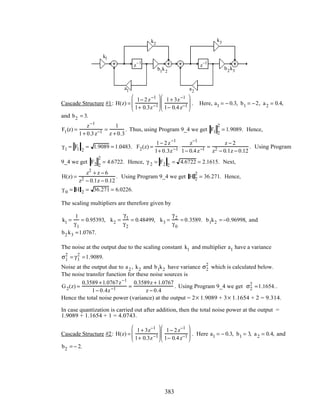
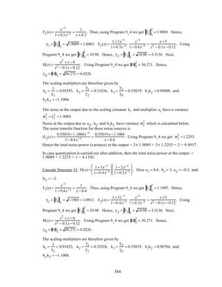
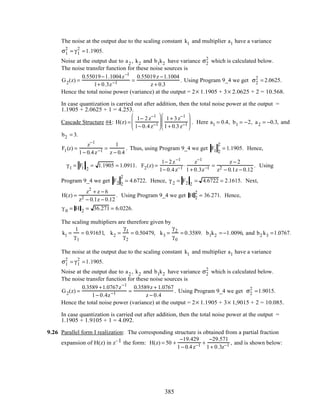
390. −19.429
−29.571
F1 (z)
F2( z)
z−1
z−1
50
0.4
−0.3
Here the scaling transfer function F1(z) for the middle branch is given by
F1(z) =
−19.429z
z − 0.4
. Hence using Program 9_4 we get, F1 2
2
= 449.39. This implies
γ1 = F1 2
= 449.39 = 21.199. Similarly, the scaling transfer function for the bottom branch
is given by F2(z) =
–29.571z
z + 0.3
. Hence using Program 9_4 we get, F2 2
2
= 960.93. This
implies γ 2 = F2 2
= 960.93 = 30.999. Finally using Program 9_4 we get, H 2
2
= 36.271.
Hence, γ 0 = H 2 = 36.271 = 6.0226. The scaled structure with noise sources is shown
below:
z
−1
z
−1
0.4
− 0.3
A
B
C
k1
k2
where A =
−19.429
γ1
= − 0.91651, B =
−29.571
γ 2
=− 0.95393, C =
50
γ0
=8.3021, k1 =
γ1
γ0
=3.5199,
and k2 =
γ2
γ0
= 5.1471.
The noise transfer function from each of the noise sources eC[n], ek1[n], and ek2[n] is
G3(z) = 1. The corresponding output noise variance is σ3
2
=1. The noise transfer function
from each of the noise sources eA[n] and ea1[n] is G1(z) =
k1
1− 0.4z−1 =
3.5199z
z − 0.4
. Using
Program 9_4 we get the corresponding output noise variance as σ1
2
=14.75. Likewise, the
noise transfer function from each of the noise sources eB[n] and ea2[n] is
386

391. G2(z) =
k2
1+ 0.3z−1 =
5.1471z
z + 0.3
. Using Program 9_4 we get the corresponding output noise
variance as σ2
2
= 29.113. Total noise variance at the output is therefore
σo
2
= 2σ1
2
+ 2σ2
2
+3σ3
2
= 2(14.75) + 2(29.113) + 3= 90.726.
Parallel form II realization: The corresponding unscaled structure is obtained from a partial
fraction expansion of H(z) in z in the form: H(z) = 1+
−7.7714
z − 0.4
+
8.8714
z + 0.3
. and is shown
below.
z
−1
z
−1
0.4
− 0.3
F1(z)
F2(z)
8.8714
− 7.7714
Here the scaling transfer function F1(z) for the middle branch is given by F1(z) = –
7.7714
z − 0.4
.
Hence using Program 9_4 we get, F1 2
2
= 71.898. This implies γ1 = F1 2
= 71.898 = 8.4793.
Similarly, the scaling transfer function for the bottom branch is given by F2(z) =
8.8714
z + 0.3
.
Hence using Program 9_4 we get, F2 2
2
= 86.485. Thus, γ 2 = F2 2
= 86.485 = 9.2998.
Finally using Program 9_4 we get, H 2
2
= 36.271. Hence, γ 0 = H 2 = 36.271 = 6.0226.
The scaled structure with noise sources is shown below:
A
B
C
k1
k2
z
−1
z
−1
0.4
− 0.3
where A =
− 7.7714
γ1
= − 0.91651, B =
8.8714
γ2
= 0.95394, C =
1
γ0
= 0.16604, k1 =
γ1
γ0
=1.4079,
k2 =
γ2
γ0
=1.5441.
387

392. The noise transfer function from each of the noise sources eC[n], ek1[n], and ek2[n] is
G3(z) = 1. The corresponding output noise variance is σ3
2
=1. The noise transfer function
from each of the noise sources eA[n] and ea1[n] is G1(z) =
k1 z−1
1− 0.4z−1 =
1.4079
z − 0.4
. Using
Program 9_4 we get the corresponding output noise variance as σ1
2
= 2.3597. Likewise, the
noise transfer function from each of the noise sources eB[n] and ea2[n] is
G2(z) =
k2 z−1
1+ 0.3z−1 =
1.5441
z + 0.3
. Using Program 9_4 we get the corresponding output noise
variance as σ2
2
= 2.62. Total noise variance at the output is therefore
σo
2
= 2σ1
2
+ 2σ2
2
+3σ3
2
= 2(2.3597)+ 2(2.62) + 3= 12.959.
For quantization of products after addition, the total output noise variance in the case of
Parallel form I structure (after scaling) is σo
2
= σ1
2
+ σ2
2
+ σ3
2
= 14.75 + 29.113+1= 44.863. and
total output noise variance in the case of Parallel form II structure (after scaling) is
σo
2
= σ1
2
+ σ2
2
+ σ3
2
= 2.3597 + 2.62 +1= 5.9797. In either case, Parallel form II structure (after
scaling) has the lowest roundoff noise variance.
9.27 H(z) =
2 + 2z−1
− 1.5z−2
1+ 0.5z−1
+ 0.06z−2 =
2z2
+ 2z − 1.5
z2
+ 0.5+ 0.06
= 2
z2
+ z − 0.75
z2
+ 0.5 + 0.06





 ..
(a) Direct Form: The unscaled structure is shown below:
y[n]
z
−1
x[n]
z
−1
2
F1(z)
–0.5
–0.06 –0.75
Scaling: F1(z) =
2
1+ 0.5z−1
+ 0.06 z−2 =
2z2
z2
+ 0.5 + 0.06
. Using Program 9_4 we get,
F1 2
2
= 5.1633. This implies, β0 =
1
F1 2
=
1
5.1633
= 0.44009. The other scaling transfer
function is H(z) =
2z2
+ 2z −1.5
z2 + 0.5+ 0.06
. Using Program 9_4 we get, H 2
2
= 10.6512. This implies
β1 =
F1 2
H 2
=
5.1633
10.6512
= 0.69625.
388

393. The scaling multipliers are therefore K = β0K = 0.44009× 2 = 0.88018,
b01 = β1 = 0.69625, b11 =1×β1 = 0.69625, and b21 = (−0.75)β1 = −0.52219.
The scaled structure with the noise sources is shown below:
K b01
b11
b21
y[n]
z
−1
x[n]
z
−1
–0.5
–0.06
e1[n] + e2[ n] + e3[n] e4[n] + e5[n] + e6[n]
G1(z)
G4(z)
Product roundoff noise analysis, quantization before addition:
G1(z) = G2(z) = G3(z) =
b01 z2 + b11z + b21
z2 + 0.5z + 0.06
. Using Program 9_4 we get,
σ1,n
2
= σ2,n
2
= σ3,n
2
= 1.2908. G4(z) = G5(z) = G6(z) = 1. This implies, σ4,n
2
= σ5,n
2
= σ6,n
2
= 1.
Hence, total normalized output noise power is σn
2
= 3×1.2908 + 3×1= 6.8725.
Product roundoff noise analysis, quantization after addition:
Here, total normalized output noise power is σn
2
= 1.2908 +1= 2.2908.
(b) Cascade Structure #1: H(z) =
2(1− 0.5z−1
)(1 +1.5z−1
)
(1+ 0.2z−1
)(1 + 0.3z−1
)
. The unscaled structure is shown
below:
F1(z)
F2(z)
2
1.5
z
−1
z
−1
− 0.3− 0.5− 0.2
Scaling: F1(z) =
2
1+ 0.2z−1 . Using Program 9_4 we get F1 2
2
= 4.1667. This implies
β0 =
1
F 2
=
1
4.1667
= 0.4899. The second scaling transfer function is
389

394. F2(z) =
2(1− 0.5z−1
)
(1+ 0.2z−1)(1+ 0.3z−1)
=
2z2
− z
z2 + 0.5z + 0.06
. Using Program 9_4 we get, F2 2
2
= 8.8896.
This implies β1 =
F1 2
F2 2
=
4.1667
8.8896
= 0.68463. The third scaling transfer function is
H(z) =
2z2
+ 2z −1.5
z2 + 0.5+ 0.06
. Using Program 9_4 we get, H 2
2
= 10.6512. This implies
β2 =
F2 2
H 2
=
8.8896
10.6512
= 0.91357.
The scaling multipliers are therefore K1 = β0K = 0.4899 × 2 = 0.9798, b01 = β1 = 0.68463,
b11 = −0.5×β1 = −0.34231, b02 = β2 = 0.91357, and b12 = 1.5 ×β2 =1.3704.
The scaled structure with the noise sources is shown below:
y[n]
z
−1
x[n]
z
−1
–0.2 –0.3
K1
b01
b11
b02
b12
e1[n] e3[n] e6[n]
e2[n] e4[n] e5[n] e6[n]
Product roundoff noise analysis, quantization before addition:
G1(z) = G2 (z) =
(0.68463 − 0.34231z−1
)(0.91357 + 1.3704 z−1
)
(1 + 0.2z−1
)(1+ 0.3z−1
)
=
0.6255z2
+ 0.6255 z − 0.4691
z2
+ 0.5z + 0.06
.
Using Program 9_4 we get σ1,n
2
= σ2,n
2
= 1.0417.
G3(z) = G4 (z) =
0.91357 +1.3704z−1
1 + 0.3z−1 =
0.91357z + 1.3704
z + 0.3
. Using Program 9_4 we get
σ3,n
2
= σ4,n
2
= 2.1553. Finally, G5(z) = G6(z) =1. This implies, σ5,n
2
= σ6,n
2
=1.
Hence, total normalized output noise power is σn
2
= 2 ×1.0417 + 2× 2.1553 + 2× 1= 8.3940.
Product roundoff noise analysis, quantization after addition:
Here, total normalized output noise power is σn
2
= 1.0417 + 2.1553 + 1= 4.1970.
(c) Cascade Structure #2: H(z) =
2(1+ 1.5z−1
)(1− 0.5z−1
)
(1+ 0.2z−1
)(1 + 0.3z−1
)
. The unscaled structure is shown
below:
390

395. F1(z)
F2(z)
2
1.5
z−1
z−1
− 0.3 − 0.5− 0.2
Scaling: F1(z) =
2
1+ 0.2z−1 . Using Program 9_4 we get F1 2
2
= 4.1667. This implies
β0 =
1
F 2
=
1
4.1667
= 0.4899. The second scaling transfer function is
F2(z) =
2(1+ 1.5z−1
)
(1+ 0.2z−1
)(1+ 0.3z−1
)
=
2z2
+ 3z
z2
+ 0.5z + 0.06
. Using Program 9_4 we get, F2 2
2
= 9.4741.
This implies β1 =
F1 2
F2 2
=
4.1667
9.4741
= 0.6632. The third scaling transfer function is
H(z) =
2z2
+ 2z −1.5
z2 + 0.5+ 0.06
. Using Program 9_4 we get, H 2
2
= 10.6512. This implies
β2 =
F2 2
H 2
=
9.4741
10.6512
= 0.9431.
The scaling multipliers are therefore K1 = β0K = 0.4899 × 2 = 0.9798, b01 = β1 = 0.6632,
b11 =1.5×β1 = 0.9948, b02 = β2 = 0.9431, and b12 = −0.5 ×β2 = −0.4716.
The scaled structure with the noise sources is shown below:
y[n]
z
−1
x[n]
z
−1
–0.2 –0.3
K1
b01
b11
b02
b12
e1[n] e3[n] e6[n]
e2[n] e4[n] e5[n] e6[n]
Product roundoff noise analysis, quantization before addition:
G1(z) = G2 (z) =
(0.6632 + 0.9948z−1
)(0.9431 − 0.4716z−1
)
(1+ 0.2z−1
)(1+ 0.3z−1
)
=
0.6255z2
+ 0.6255z − 0.4691
z2
+ 0.5z + 0.06
.
Using Program 9_4 we get σ1,n
2
= σ2,n
2
= 1.0417.
391

396. G3(z) = G4 (z) =
0.9431− 0.4716 z−1
1+ 0.3z−1 =
0.9431z − 0.4716
z + 0.3
. Using Program 9_4 we get
σ3,n
2
= σ4,n
2
= 1.5151. Finally, G5(z) = G6(z) =1. This implies, σ5,n
2
= σ6,n
2
=1.
Hence, total normalized output noise power is σn
2
= 2 × 0.1.0417 + 2×1.5151+ 2× 1= 7.1136.
Product roundoff noise analysis, quantization after addition:
Here, total normalized output noise power is σn
2
= 0.1.0417 + 1.5151 + 1= 3.5568.
Hence, the scaled direct form realization has the smallest roundoff noise in both cases.
9.28 The noise model for the allpass structure is shown below
x[n] z−1
v[n]
w[n]
–1
r[n]
e[n]
d i
y[n]
Analysis yields W(z) = E(z) + diV(z), R(z) = X(z) – W(z), V(z) = X(z) + z–1R(z), and
Y(z) = W(z) + z–1R(z).
To determine the noise transfer function we set X(z) = 0 in the above equations. This leads to
R(z) = – W(z), V(z) = z–1R(z) = – z–1W(z), and hence W(z) = E(z) – diz–1W(z) or
E(z) = (1 + diz–1)W(z). As a result, Y(z) = W(z) – z–1W(z) = (1 – z–1)W(z). Consequently,
the noise transfer function is given by
G(z) =
Y(z)
E(z)
=
1– z–1
1+ di
z–1 =
z –1
z + di
=1+
–(1+ di )
z + di
.
Thus σe
2
=1+
(1+ di)2
1− di
2 =
2
1− di
.
(b) Let G1(z) be the noise transfer function for d1, G2(z) be the noise transfer function for d2
and G3(z) be the noise transfer function for d3 then
G1(z) =
z −1
z + d1
A2(z), G2(z) =
z −1
z + d2
and G3(z) =
z −1
z + d3
. From the results of part (a) it
follows that the noise variances due to d1, d2 and d3 are given by
σk
2
=
2
1− dk
for k = 1, 2, 3. Hence the total noise power at the output is given by
σ2
=
2
1− d1
+
2
1− d2
+
2
1− d3
.
392

397. 9.29 Let the total noise power at the output of G(z) due to product-off be given by σG
2
. Asuming
a total of L multipliers in the realization of G(z) we get σG
2
= kl
1
2π
Gl (ejω
)
2
dω
0
2π
∫









l =1
L
∑ where
Gl (z) denotes the noise transfer function due to l -th noise source in G(z). Now if each delay is
replaced by two delays then each of the noise transfer function becomes Gl (e2jω
). Thus the
total noise power at the output due to noise sources in G(z2) is given by ˆσ G
2
=
kl
1
2π
Gl (e2jω
)
2
dω
0
2π
∫









l =1
L
∑ . Replacing ω by ˆω / 2 in the integral we get ˆσ G
2
=
kl
1
2π
Gl (ej ˆω
)
2 1
2( )d ˆω
0
4π
∫









l =1
L
∑ =
1
2
kl
1
2π
Gl (e j ˆω
)
2
d ˆω
0
4π
∫









l =1
L
∑ = σG
2
. Since
1
2π
Gl (ejω
)
2
A(ejω
)
2
dω
0
2π
∫ =
1
2π
Gl (ejω
)
2
dω
0
2π
∫ , the total noise power at the output of the
cascade is still equal to σ0
2
.
9.30 For the first factor in the numerator there are R possible choices of factors. Once this factor has
been choosen, there are R – 1 choices for the next factor and continuing further we get that the
total number of possible ways in which the factors in the numerator can be generated equal to
R(R −1)(R − 2)L2 ×1= R!. Similarly the total number of ways in which the factors in the
denominator can be generated = R!. Since the numerator and denominator are generated
independent of each other hence the total number of possible realizations are N = (R!)(R!) =
(R!)2 .
9.31 (a) First we pair the poles closest to the unit circle with their nearest zeros resulting in the
second-order section Ha(z) =
z2
+ 0.2z + 0.9
z2 + 0.1z + 0.8
. Next, the poles that are closest to the poles of
Ha(z) are matched with their nearest zeros resulting in the second-order section Hb(z) =
z2
+ 0.3z + 0.5
z2 + 0.2z + 0.4
. Finally, the remaining poles and zeros are matched yielding the second-order
section Hc(z) =
z2
+ 0.8z + 0.2
z2 + 0.6z + 0.3
.
For odering the sections to yield the smallest peak output noise due to product round-off under
an L2-scaling rule, the sections should be placed from most peaked to least peaked as shown
below.
Ha (z) H b(z) Hc (z)
For odering the sections to yield the smallest peak output noise power due to product round-off
under an L∞-scaling rule, the sections should be placed from least peaked to most peaked as
shown below.
393

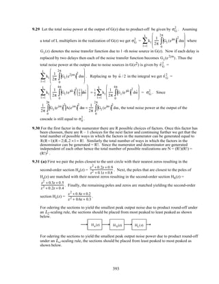
398. Ha(z)Hb (z)Hc(z)
(b) The poles closest to the unit circle is given by the denominator (z2 – 0.2z + 0.9), the next
closer pole is given by the factor (z + 0.9), followed by the factor (z2 + 0.4z + 0.7) and finally
the factor (z + 0.2). Pairing these poles with their closest zeros we get the following pairings:
Ha(z) =
z2
+ 0.1z + 0.7
z2 − 0.2z + 0.9
, Hb(z) =
z +1.1
z + 0.9
, Hc(z) =
z2
+ 0.5z + 0.6
z2 + 0.4z + 0.7
and Hd(z) =
z + 0.3
z + 0.2
.
For odering the sections to yield the smallest peak output noise due to product round-off under
an L2-scaling rule, the sections should be placed from most peaked to least peaked as shown
below.
Hc (z)Ha (z) Hb(z) Hd (z)
For odering the sections to yield the smallest peak output noise power due to product round-off
under an L∞-scaling rule, the sections should be placed from least peaked to most peaked as
shown below.
Hc(z) Ha (z)Hb (z)Hd (z)
9.32 SNR =
σx
2
σ0
2 . After scaling σx changes to Kσx where K is given by Eq. (9.150).
Therefore SNR =
σx
2 1− α( )
2
σ0
2 .
(i) For uniform density function σx
2
=
1
2
x2
dx
−1
1
∫ =
1
3
.
Thus SNR =
1− α( )
2
3σ0
2 . With b = 12 σ0
2
=
2
−24
12
= 4.967× 10–9 and α = 0.95,
Hence SNRdB = 10 log10
1− α( )
2
3σ0
2








= 52.24 dB.
(ii) For Gaussian input with σx
2
=
1
9
. Hence SNR =
1− α( )
2
9σ0
2 . Again with b = 12 and
α = 0.95, SNRdB = 10 log10
1− α( )
2
9σ0
2








= 47.97 dB.
(iii) For a sinusoidal input of known frequency, i.e. x[n] = sin(ω0n).
In this case average power =σx
2
=
1
2
. Hence SNR =
(1− α )2σx
2
σ0
2 =
(1− α )2
2σ0
2 .
394

399. Therefore SNRdB = 10 log10
(1− α )2
2σ0
2








= 69.91 dB.
9.33 (a) HLP(z) =
1
2
1+ A1(z){ } where A1(z) =
−α + z−1
1−αz−1 .
Hence HLP (e jω
)
2
=
1− α
2






2 2 1+ cos(ω)( )
1− 2α cos(ω)+ α2 .
Proving
∂HLP(ejω
)
∂α
ω=0
= 0 is equivalent to proving
∂HLP(ejω
)
2
∂α
ω=0
= 0. Now
∂HLP(ejω
)
2
∂α
= −
1− α
2
2(1+ cos(ω))
1− 2αcos(ω) + α2 −
1− α
2






2
2(1+ cos(ω))(−2cos(ω)+ α)
1− 2α cos(ω)+ α2 .
Thus,
∂HLP(ejω
)
2
∂α
ω=0
=
−2
1− α
+
2
1− α
= 0.
(b) HHP(z) =
1
2
1− A1(z){ } where A1(z) =
−α + z−1
1−αz−1 .
Hence HHP (ejω
)
2
=
1+ α
2






2
2(1− cos(ω))
1− 2αcos(ω)+ α2 .
Now
∂HHP(ejω
)
2
∂α
= −
1+ α
2
2(1− cos(ω))
1− 2αcos(ω) + α2 −
1+ α
2






2
2(1− cos(ω))(−2cos(ω)+ α)
1− 2α cos(ω)+ α2 .
Thus,
∂HHP(ejω
)
2
∂α
ω=π
=
−2
1+ α
+
2
1+ α
= 0.
9.34 (a) HBP(z) =
1
2
1− A2 (z){ } where A2(z) =
α − β(1+ α)z−1
+ z−2
1− β(1+ α)z−1 + αz−2 , with α and β being real.
Therefore, HBP(ejω
)
2
=
1− α
2






2
2(1− cos(ω))
1+ β2 (1+ α)2 + α2 + 2αcos(2ω)− 2β(1+ α)2 cos(ω)





 . Now,
∂HBP(ejω
)
2
∂α
=
−2
1− α






1− α
2






2
2(1− cos(ω))
1+ β2 (1+ α)2 + α2 + 2αcos(2ω)− 2β(1+ α)2 cos(ω)






+
1−α
2






2
2(1− cos(ω))
1+β2(1+ α)2 + α2 + 2α cos(2ω) − 2β(1+ α)2 cos(ω)





 ×
2β2
(1+ α)+ 2α + 2cos(2ω)− 4β(1+ α)cos(ω)
1+ β2 (1+ α)2 + α2 + 2αcos(2ω)− 2β(1+ α)2 cos(ω)





 .
395

400. Using the fact β = cos(ω0) we get
∂HBP(ejω
)
2
∂α
ω=ω0
=
−2
1− α
−
2β2
+ 2α − 2 − 2αβ2
( )
1+ α2 − 2α + 2αβ2 − β2 − α2β2
=
−2
1− α
+
2
1− α
= 0.
Similarly,
∂HBP(ejω
)
2
∂β
=
1− α
2






2
2(1− cos(ω))
1+ β2 (1+ α)2 + α2 + 2αcos(2ω)− 2β(1+ α)2 cos(ω)





 ×
−
2β(1+ α)2
− 2(1+ α)2
cos(ω)
1+ β2(1+ α)2 + α2 + 2α cos(2ω)− 2β(1+ α)2 cos(ω)





 .
Again using the fact that β = cos(ω0) it can be seen that
∂HBP(ejω
)
2
∂β
ω=ω0
= 0.
(b) For bandstop filters HBS(z) =
1
2
1+ A2 (z){ } where A2(z) is as given in (a). Thus
HBS(e jω
)
2
=
1+ α
2






2
4β2
+ 2 + 2cos(2ω)− 8βcos(ω)
1+ β2 (1+ α)2 + α2 + 2αcos(2ω)− 2β(1+ α)2 cos(ω)





 . Thus,
∂HBS(ejω
)
2
∂α
=
1+ α
2






4β2
+ 2 + 2cos(2ω)− 8βcos(ω)
1+ β2(1+ α)2 + α2 + 2α cos(2ω)− 2β(1+ α)2 cos(ω)






–
1+ α
2






2
4β2
+ 2 + 2cos(2ω)− 8βcos(ω)
1+ β2 (1+ α)2 + α2 + 2αcos(2ω)− 2β(1+ α)2 cos(ω)





 × ×
2(1+ α)β2
+ 2α + 2cos(2ω)− 4β(1+ α)cos(ω)
1+ β2 (1+ α)2 + α2 + 2αcos(2ω)− 2β(1+ α)2 cos(ω)





 .
Substituting β = cos(ω0) it can be seen that
∂HBS(ejω
)
2
∂α
ω=0
=
2
1− α
−
1+ α
2






2
2(1+ α)(β +1)2
(1+ α)2 (β +1)2





 = 0.
Similarly,
∂HBS(ejω
)
2
∂α
ω=π
=
2
1− α





 −
1+ α
2






2
2(1+ α)(β + 1)2
(1+ α)2(β + 1)2





 = 0.
Now,
∂HBS(ejω
)
2
∂β
=
1+ α
2






2
8β −8cos(ω)
1+ β2(1+ α)2 + α2 + 2α cos(2ω)− 2β(1+ α)2 cos(ω)






−
1+α
2






2
4β2
+ 2 + 2cos(2ω) − 8β cos(ω)
1+β2(1+ α)2 + α2 + 2α cos(2ω) − 2β(1+ α)2 cos(ω)





 ×
(1+ α)2
2(β − cos(ω)
1+ β2 (1+ α)2 + α2 + 2αcos(2ω)− 2β(1+ α)2 cos(ω)





 .
Again substituting β = cos(ω0) it can be seen that
396

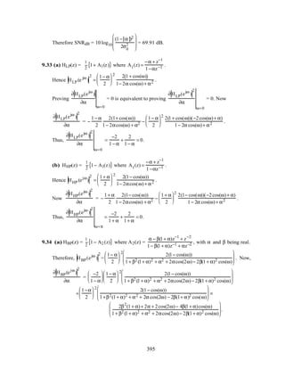
401. ∂HBS(ejω
)
2
∂β
ω=0
= 0 and also
∂HBS(ejω
)
2
∂β
ω=π
=0.
9.35 For a BR transfer function G(z) realized in a parallel allpass form, its power-complementary
transfer funnction H(z) is also BR atisfying the condition G(ejω
)
2
= 1− H(ejω
)
2
. Let ω = ωo
be a frequenncy where G(ejω
) is a maximum, i.e. G(ejωo ) = 1. Then, it follows that
H(ejωo ) = 0. From the power-complementary condition it follows that
2 G(ejω
)
∂G(e jω
)
∂ω
= −2 H(e jω
)
∂H(ejω
)
∂ω
. Therefore at ω = ωo ,
G(ejωo )
∂G(ejω
)
∂ω
ω=ωo
= − H(ejωo )
∂H(ejω
)
∂ω
ω=ωo
, or
∂G(ejω
)
∂ω
ω=ωo
= 0 whether or not
∂H(ejω
)
∂ω
ω=ωo
= 0. Hence, lowpassband sensitivity of G(z) does not necessarily imply low
stopband sensitivity of H(z).
9.36 Without error feedback
The transfer function H(z) of the structure without feedback is given by
H(z) =
1
1+ α1
z−1 + α1
z−1 =
1
1− 2r cosθz−1 + r2z−1 , where r = 1 – ε.
The corresponding impulse response h[n] is given by h[n] =
rn
sin(n +1)θ
sinθ
⋅µ[n].
To keep y[n] from overflowing we must insert a multiplier of value
1
L
at the input where
L = h[n]
n=0
∞
∑ . From Eq. (9.163) we get
1
(1− r)2(1− 2rcosθ + r2)
≤ L2
≤
16
π2(1− r)2 sin2 θ
. (24)
The quantization noise model for H(z) is as shown below:
z–1
z–1
x[n] y[n]
e[n]
2 r cosθ
– r
2
1
L
397

402. The output noise power is given by σn
2
= σe
2
h[n]
2
n=0
∞
∑ =
1+ r2
1− r2 ⋅
1
r4 − 2 r2 cosθ+ 1
⋅σe
2
The output signal power, assuming an input signal of variance σx
2
is given by
σy
2
=
σx
2
L2 h[n]
2
n=0
∞
∑ . Hence, the SNR is given by SNR =
σy
2
σn
2 =
σx
2
L2σe
2 . For a (b+1)-bit signed
representation, σe
2
=
2−2b
12
. Hence, SNR =
S
N
=
12σx
2
L2 2−2b . Therefore, from the inequality of Eq.
(24) we get
2−2b
12 σx
2(1− r)2 (1− 2r cosθ+ r2 )
≤
N
S
≤
16 × 2−2b
12 σx
2π2(1− r)2 sin2 θ
.
(a) For an WSS uniformly distributed input between [– 1, 1], σx
2
=
1
3
. Hence,
2−2b
4(1− r)2 (1− 2 rcosθ + r2 )
≤
N
S
≤
4
π2
2−2b
(1− r)2 sin2 θ
.
If ε → 0, and θ → 0, then (1− r)2
→ ε2
, cos2θ =1− 2sin2
θ ≅ 1− 2θ2
, and sin2
θ ≅ θ2
.
In this case we have
2−2b
4ε2 (ε2 + 4θ2)
≤
N
S
≤
2−2b
π2ε2θ2 .
(b) For an input with a Gaussian distribution between [– 1, 1], σx =
1
3
.
In this case we have 3
2−2b
4ε2(ε2 + 4θ2)
≤
N
S
≤
3
π2
2−2b
ε2θ2 .
(c) For a sinusoidal input between [– 1, 1] of known frequency ωo , σx
2
=
1
2
.
The output noise variance here is therefore σn
2
= σe
2
h[n]
2
n=0
∞
∑ =
2−2b
12
⋅
1+ r2
1− r2 ⋅
1
r4 − 2r2 cos2θ +1
.
Thus,
N
S
=
1+ r2
1− r2 ⋅
1
6 r4 − 2r2 cos2θ +1( )
=
2−2b
24ε ε2 + θ2
( )
≅
2−2b
24 εθ2 .
With error feedback
G(z) =
1− 2z−1
+ z−1
1− 2 rcosθz−1 + r2z−1 =
z2
− 2z +1
z2 − 2r cosθz + r2 = 1+
2(r cosθ −1)z +1− r2
z2 − 2r cosθz + r2 .
Thus, G
2
= 1+
4(1− rcosθ)2
+ (1− r2
)2
( )(1− r4
)+ 8r cosθ(1− r2
)2
(r cosθ −1)
(1− r2)2 + 2r2(4r2 cos2 θ)− 4(1+ r4)r2 cos2 θ
For r = 1− ε with ε → 0, and θ → 0, we get after some manipulation G
2
= 1+
θ4
4ε(ε2 +θ2)
,
and σn
2
= σe
2
G
2
.
Now L2 remains the same as before since it depends only upon the denominator. Also the
overall transfer function of the structure remains the same as before. The output noise power
398

403. with error feedback is thus ˆN = σe
2
G
2
, whereas, the output noise power without error feedback
is N = σe
2
H
2
. Hence,
ˆN
N
=
G 2
H 2 .
Now, G
2
= 1+
θ4
4ε(ε2 +θ2)
, Since θ >> ε, G
2
≅
θ4
4εθ2 =
θ2
4ε
.
Also, H
2
=
1+ r2
1− r2 ⋅
1
r4 − 2r2 cos2 θ +1
=
1+ (1− ε)2
1− (1− ε)2 ⋅
1
(1− ε)4 − 2(1− ε)2(1− 2θ2 )+1
≈
1
4ε(θ2 + ε2 )
≈
1
4εθ2 .
Thus,
ˆN
N
≅ θ4
. As a result, with error feedback, the
N
S
ratio gets multiplied by θ4
.
(a) input with uniform density:
2−2b
θ2
16ε2 ≤
N
S
≤
θ2
π2
2−2b
ε2
(b) Wide-sense stationary, Gaussian density, white:
2−2b
3θ2
16ε2 ≤
N
S
≤
3θ2
π2
2−2b
ε2
(c) sinusoid with known frequency:
N
S
=
2−2b
θ2
24 ε
9.37 The coupled form with error feedback is shown below:
z−1
z
−1
z−1
z
−1
α
β
δ
γ
Q
Q
λ1
λ2
–
+
+
–
e1[n]
e2[n]
v2[n]
v1[n]
y[n]
u[n]
Analysis yields V1(z) = λ1z−1
E1(z) + δz−1
Y(z) + γ z−1
U(z), E1(z) = Y(z) − V1(z),
V2 (z) = λ2z−1
E2(z) + βz−1
Y(z) + α z−1
U(z), and E2(z) = Y(z) − V2 (z). Eliminating
U1(z), V1(z), U2 (z),and V2 (z) from these equations we arrive at the noise transfer functions
G1(z) =
Y(z)
E1(z) E2 (z)=0
=
(1− α z−1
)(1+ λ1 z−1
)
1− (α + δ)z−1
+ (αδ − βγ)z−2 , and
G2(z) =
Y(z)
E2(z) E1(z)=0
=
γ z−1
(1+ λ2 z−1
)
1− (α + δ)z−1
+ (αδ − βγ)z−2 . The total output noise
399

404. power is thus given by σo
2
= G1 2
2
σe1
2
+ G2 2
2
σe2
2
. Hence, the output noise power, for a
lowpass filter design, can be reduced by placing zeros of the noise transfer functions in the
passband. For each of the noise transfer functions given above, we can only place a zero at z =
1 by choosing λi = −1, i = 1, 2,
Using the notations b = −(α + δ) and d = αδ − βγ we rewrite the noise transfer functions as
G1(z) =
z2
− (1 + α)z + α
z2
+ bz + d
= 1+
−(1+ α + b) + (α − d)
z2
+ bz + d
, and G2(z) =
γ z − γ
z2
+ bz + d
. Using Table
9.4 we obtain G1 2
2
= 1+
(1+ α + b)2
+ (α − d)2
[ ](1− d2
) + 2(1+ α + b)(α − d)(1− d)
(1− d2
)2
+ 2d b2
− (1+ d2
)b2 , and
G2 2
2
=
2γ2
(1− d2
)
(1− d2
)2
+ 2d b2
− (1+ d2
)b2 .
9.38 The Kingsbury structure with error feedback is shown below:
–
+
e1[n] e2[n]
v2[n]v1[n] y[n]
z
−1
z−1
z
−1
z
−1
Q Q
λ1 λ 2
z
−1
Q
λ3
k1 k2
− k1u1[n]
u2[n] u3[n]
v3[n]
e3[n]
–
+
–
+
Analysis yields: V1(z) = k1Y(z) + z−1
U1(z) + λ1z−1
E1(z), E1(z) = U1(z) − V1(z),
V2 (z) = k2Y(z) + U1(z) + λ2z−1
E2(z), E2(z) = U2(z) − V2 (z),
V3(z) = Y(z) − k1U2(z) + λ3z−1
E3 (z), E3(z) = U3(z) − V3(z), and Y(z) = z−1
U1(z). Eliminating
U1(z), V1(z), U2 (z), V2(z), U3(z) and V3(z) from these equations we get
G1(z) =
Y(z)
E1(z) E2 (z)=E3(z)=0
=
− k1z−1
(1+ λ1z−1
)
1− 2 − k1(k1 + k2 )[ ]z−1
+ (1− k1k2 )z−2 ,
G2(z) =
Y(z)
E2(z) E1(z)=E3(z)=0
=
− k1z−1
(1− z−1
)(1+ λ2z−1
)
1− 2 − k1(k1 + k2 )[ ]z−1
+ (1 − k1k2 )z−2 , and
G3(z) =
Y(z)
E3(z) E1(z)=E2(z)=0
=
z−1
(1− z−1
)(1+ λ3z−1
)
1− 2 − k1(k1 + k2 )[ ]z−1
+ (1− k1k2 )z−2 . The total output noise
power is thus given by σo
2
= G1 2
2
σe1
2
+ G2 2
2
σe2
2
+ G3 2
2
σe3
2
. Hence, the output noise power,
for a lowpass filter design, can be reduced by placing zeros of the noise transfer functions in
the passband. For each of the noise transfer functions given above, we can only place a zero at
z = 1 by choosing λi = −1, i = 1, 2, 3, in which case, using the notations b = −[2 − k1(k1 + k2 )],
and d =1− k1k2. the noise transfer functions reduce to G1(z) =
− k1z−1
(1− z−1
)
1+ bz−1
+ dz−2 =
− k1z + k1
z2
+ bz + d
,
400

405. G2(z) =
−k1z−1
(1− z−1
)
1+ bz−1
+ dz−2 =
− k1(z2
− 2z + 1)
z(z2
+ bz + d)
=
− k1A
z
+
−k1(Cz + D)
z2
+ bz + d
and
G3(z) =
z−1
(1− z−1
)2
1+ bz−1
+ dz−2 =
z2
− 2z + 1
z(z2
+ bz + d)
=
A
z
+
C z + D
z2
+ bz + d
where A =
1
d
, C = 1−
1
d
, and
D = − 2 +
b
d





 . Using Table 9_4 we then obtain G1 2
2
= k1
2 2(1− d2
) − 2(1− d)b
(1− d2
)2
+ 2d b2
− (1+ d2
)b2 ,
G3 2
2
= A2
+ 2BC +
(C2
+ D2
)(1− d2
) − 2C D(1− d)b
(1− d2
)2
+ 2db2
− (1+ d2
)b2 , and G2 2
2
= k1
2
G3 2
2
.
9.39 The transfer function of the coupled-form structure shown below is given by Eq. (9.42) where
α = δ = r cos(θ) and β = −γ = rsin(θ). Analysis yields
x[n] y[n]
z–1
z–1
α
β
γ
δ
s1[n +1]
s2[n +1]
s1[n +1]= α x[n]+ s1[n]( )+βs2[n] and s2[n +1] = γ x[n]+ s1[n]( )+ δs2[n]. Rewriting these
equations in matrix form we get
s1[n +1]
s2[n +1]





 =
α β
γ δ






s1[n]
s2[n]





 +
α
γ



x[n]
Thus A =
α β
γ δ





 . Therefore, ATA =
α γ
β δ




α β
γ δ





 =
α2
+ γ2
αβ + γδ
αβ + γδ β2
+ δ2








=
r2 0
0 r2





.
Likewise, AAT = α β
γ δ






α γ
β δ



 =
α2
+ β2
αγ + βδ
αγ + βδ γ2
+δ2








=
r2 0
0 r2





.
Thus A is of normal form and hence, the structure will not support limit cycles.
9.40 The transfer function of the modified coupled-form structure shown below is given by
x[n] y[n]z–1 z–1
c c
d d
s1[n +1] s2[n +1]
–1
s1[n +1]= cds1[n]−cs2[n]+ x[n], s2[n +1] = cs1[n]+ c ds2[n], and y[n] = cs2[n].
In matrix form these equations can be written as
s1[n +1]
s2[n +1]





 =
cd −c
c cd




s1[n]
s2[n]





 +
1
0



 x[n], and y[n] = 0 c[ ]
s1[n]
s2[n]





 + [0]x[n]. Thus,
401

406. A =
cd −c
c cd



 . Now, in the z-domain the equations describing the structure are
zS1(z) = cdS1(z)− cS2(z)+ X(z), zS2(z) = c S1(z) + cdS2 (z), and Y(z) = c S2(z). From the
equation on the left we get (z − cd)S1(z) = −cS2 (z) + X(z) and from the equation on the right we
get (z − cd)S2(z) = cS1(z). Eliminating S1(z) we arrive at S2 (z) =
cX(z)
z2 − 2cdz + c2d2 + c2 . Hence
H(z) =
Y(z)
X(z)
=
c2
z2 − 2cdz + c2(1+ d2 )
.
Comparing denominator of H(z) with the denominator z2
− 2 rcosθz + r2
of a second order
transfer function we get c = r sinθ, d = cotθ . Then A =
cd −c
c cd



 =
rcosθ −r sinθ
r sinθ r cosθ



.
Thus ATA =
r
2
0
0 r
2





, and similarly AAT =
r
2
0
0 r
2





. Since for stability r < 1,
A is normal form matrix, and thus the structure does not support limit cycles.
9.41 A block-diagram representation of a digital filter structure based on the state-space description
given by Eqs. (9.200) and (9.201) is as shown below.
s[n +1]B
A C
z
−1
I
s[n]
x[n]
y[n]
D
The feedback loop under zero-input conditions is thus as indicated below:
A
v[n +1]
s[n + 1]
s[n]
z−1
I
Q
Hence, under zero-input conditions we have
v[n +1]= As[n],
s[n +1] = Q v[n +1]( ).
The quadratic function f(s[n]) = sT[n] D s[n], where D is a positive-definite diagonal matrix, is
related to the power stored in the delays. The changes in this quantity can provide information
regarding oscillations under zero-input conditions:
∆f(s[n]) = f(s[n +1]) − f(s[n]) = − sT
[n]⋅D ⋅s[n]+ sT
[n +1]⋅D⋅s[n +1]
= − sT
[n]⋅D ⋅s[n]+ sT
[n +1]⋅D⋅s[n +1]+ vT
[n +1]⋅D⋅v[n +1]− vT
[n+ 1]⋅D⋅v[n +1]
402

407. = − sT
[n]⋅D⋅s[n]+ sT
[n +1]⋅AT
⋅D⋅A⋅s[n+ 1]− vk
2
[n+ 1]−Q (vk[n +1])2
( )k =1
N
∑ dkk
= − sT
[n] D − AT
⋅D⋅A( )s[n]− vk
2
[n+ 1]−Q (vk[n +1])2
( )k =1
N
∑ dkk .
Now if sT
[n] D− AT
DA( )s[n] ≥ 0,and vk[n] are quantized such that Q (vk[n +1]) ≤ vk[n +1],
(i.e. using a passive quantizer), then the power stored in the delays will not increase with
increasing n. So under passive quantization, limit cycles will be eliminated if
sT
[n] D− AT
DA( )s[n] ≥ 0, or D − AT
DA is positive-definite. For second order stable IIR
filters, eigen values of A = [aij] are less than 1. This condition is satisfied if
a12a21 ≥ 0,
or, a12a21 < 0 and a11 − a22 + det(A) ≤1.
For the given structure,
A =
α1 α1 +1
α2 −1 α2





, B =
α1 − β1
α2
− β2





, C = 1 1[ ], and D = 1.
The transfer function of the filter is given by
H(z) =
z2 − (β1 + β2 )z + (1+ β1 −β2)
z2 −(α1
+ α2
)z + (1+ α1
− α2
)
.
The filter is stable if 1+ α1 − α2 < 1, and α1 + α2 <1+ (1+ α1 − α2), or equivalently, if
α1 − α2 < 0, and α1 + α2 < 2 + α1 −α2.
Now, a1a2 = (α1 +1)(α2 −1) =
1
4
(α1 + α2 )2
− (2 + α1 − α2)2
[ ], and since,
(α1 + α2 )2
< (2 + α1 − α2 )2
, a12a21 < 0.
Next, a11 − a22 + det(A) = α1 − α2 + α1α2 − (α1 +1)(α2 −1)
= = − (α1 − α2 ) + α1α2 − (α1α2 + α2 − α1 −1) = 1.
Hence, the structure does not support zero-input limit cycles.
9.42 From Section 8.3.1 we know that each computation of a DFT sample requires 2N + 4 real
multiplications. Assuming that quantization noise generated from each multiplier is independent
of the noise generated from other multipliers, we get σr
2
= (2N + 4)σ0
2
=
2−2b
(N + 2)
6
.
9.43 SNR =
22b
N2 . Hence, an SNR of 25 dB implies
22b
N2 = 102.5 or
b =
1
2
log2 (10)2.5
× (512)2
( )= 13.1524. Therefore b = 14 bits should be chosen to get an SNR of
25 dB. Therefore number of bits required for each sample = 14 + 1 = 15.
9.44 Let N = 2ν
. Consider the mth stage. The output sees 4(2ν−m
) noise sources from the mth stage.
Each noise source has a variance reduction by a factor of
1
4( )
ν−m
due to multiplication by
1
2
at
each stage till the output. Hence the total noise variance at the output due to the noises injected
in the mth stage is 4 2ν−m
( ) 2−2(ν−m)
( )σ0
2
.
403

408. Therefore the total noise variance at the output =σ2
= 4 2ν−m
( )2−2(ν−m)
( )σ0
2
m=1
ν
∑
4σ0
2
2−ν
2m
m=1
ν
∑ = 4
2−2b
12
2−ν 2(2ν
−1)
2 −1
=
2
3
2−2b
(1− 2−ν
) ≈
2
3
2−2b
for large N.
9.45 SNR =
22b
2N
. Hence b =
1
2
log2 (10)2.5
× 2 × 512( ) = 8.652.
Hence we choose b + 1 = 10 bits per sample to get an SNR of 25 dB.
M9.1 % This is the function to obtain the pole distribution
% plot of a second order transfer function with a denominator
% of the form Z*Z - KZ + L. For stability 0 < L < 1 and
% abs(K) < 1+L so the range of K is (-2,2).
% for a b-bit wordlength, 1 bit is reserved for the sign
% as the coefficients are sorted in the sign magnitude form.
% Both L and the K are quantizd to b-1 bits.
%
function[]=pole_plot(bits);
%
% This part prints the unit circle for reference
%
z = [0 1];
p = [0 1];
zplane(z,p);
hold;
axis([-1 1 -1 1]);
%
% One bit is kept for the sign so effectively for the
quantization
% the remaining number of bits is bits-1
%
bits = bits-1;
%
% The quantization step.
%
step = power(2,-bits);
for index_1 = 0:1:(power(2,bits)-1)
L = index_1*step;
for index_2 = -(power(2,bits)-1):1:(power(2,bits)-1)
K = 2*index_2*step;
p1 = (-K+(sqrt(K*K-4*L)))/2;
p2 = (-K-(sqrt(K*K-4*L)))/2;
if abs(p1) < 1
if (imag(p1) ~= 0)
plot(p1,'.');
plot (p2,'.');
end
end
end
end
hold;
M9.2 The pole-distribution plot of the second-order Direct Form structure is obatined by running
the MATLAB program given in Exercise M9.1. Running this program using the statement
pole_plot(5) yields the following plot.
404

409. -1 -0.5 0 0.5 1
-1
-0.5
0
0.5
1
Real part
For plotting the pole distribution of the Kingsbury structure, we use the following MATLAB
program:
% This is the function to obtain the pole distribution plot
of the Kingsbury
% structure. Here, the transfer function has a denominator
of the form
% Z*Z - (2 - k1*k2 - k1*k1)Z + (1 - k1*k2) where the k1 and
k2 are the
% multiplier coefficients of the structure.
% For stability of the structure the range of k1 is (-2,2)
and the range
% of k2 is such that 0 < k1*k2 < 2; Hence k2 can take any
value.
% In this program the range of k1 is taken to be (-2,2) and
the range of
% k2 is also (-2,2). The wordlength is specified by the
argument "bits"
% of the function.
%
function[] = pole_plot_kb(bits);
%
% This part prints the unit circle for reference
%
z = [0 1];
p = [0 1];
zplane(z,p);
hold;
axis([-1 1 -1 1]);
%
% The numbers are stored in the sign-magnitude form so one
bit is
% reserved for the sign. Hence for the quantization, the
available bits
% = bits - 1
%
bits = bits-1;
step = power(2,-bits);
% This part of the program finds out the various possible
combinations
405

410. % of the quantized values of k1 and k2. with this set of
values of k1
% and k2, a set of transefer functions is possible and hence
a set of
% poles is possible. The possible values of poles within the
stability
% region thus obtained are plotted with the help of the plot
command.
%
for index_1 = -(power(2,bits)-1):1:(power(2,bits)-1)
k1 = 2*index_1*step;
for index_2 = -(power(2,bits)-1):1:(power(2,bits)-1)
k2 = 2*index_2*step;
if (k1*k2 < 2)
if (k1*k2 > 0)
if (k1*k1 < 4-2*k1*k2)
c = 1 - k1*k2;
b = -(2 - k1*k2 - k1*k1);
p1 = (- b + (sqrt(b*b-4*c)))/2;
p2 = (-b - (sqrt(b*b-4*c)))/2;
if (imag(p1) ~= 0)
if (real(p1) ~= 0)
if (abs(p1) < 1)
plot(p1,'.');
end
end
end
if (imag(p2) ~= 0)
if (real(p2) ~= 0)
if (abs(p2) < 1)
plot(p2,'.');
end
end
end
end
end
end
end
end
hold;
Running this program using the statement pole_plot_kb(6) yields the following plot.
-1 -0.5 0 0.5 1
-1
-0.5
0
0.5
1
Real part
406

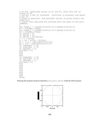
411. M9.3
0 0.2 0.4 0.6 0.8 1
-80
-60
-40
-20
0
ω/π
unquantized
quantized
M9.4 N = 5; wn = 0.45; Rp = 0.5; Rs = 45;
[B,A] = ellip(N,Rp,Rs,wn);
zplane(B,A);
z = cplxpair(roots(B)); p = cplxpair(roots(A));
disp('Factors for the numerator');
const = B(1)/A(1);
k = 1;
while k <= length(z),
if(imag(z(k)) ~=0)
factor = [1 -2*real(z(k)) abs(z(k))^2]
k = k+2;
else
factor = [1 -z(k)]
k = k+1;
end
end
disp('Factors for the denominator');
k = 1;
while k <= length(p),
if(imag(p(k)) ~=0)
factor = [1 -2*real(p(k)) abs(p(k))^2]
k = k+2;
else
factor = [1 -p(k)]
k = k+1;
end
end
sos = zp2sos(z,p,const)
The above program yields
Factors for the numerator
factor =
1.0000e+00 1.0358e+00 1.0000e+00
factor =
1.0000e+00 3.7748e-01 1.0000e+00
factor =
1.0000e+00 1.0000e+00
407

412. Factors for the denominator
factor =
1.0000e+00 -2.6433e-01 8.6522e-01
factor =
1.0000e+00 -5.8090e-01 5.0030e-01
factor =
1.0000e+00 -4.4817e-01
Hence H(z) =
1+ 1.0358z−1
+ z−2
1− 0.26433z−1 + 0.86522z−2






1+ 0.37748z−1
+ z−2
1− 0.5809z−1 + 0.5003z−2






1+ z−1
1− 0.44817z−1





 .
Note that the ordering has no effect if L∞ − scaling is used.
-1 -0.5 0 0.5 1
-1
-0.5
0
0.5
1
Real part
1
1
1
1
2
2
2
2
3 3
sos =
2.7591e-01 2.7591e-01 0 1.0000e+00 -4.4817e-01 0
3.0285e-01 3.1370e-01 3.0285e-01 1.0000e+00 -5.8090e-01
5.0030e-01
6.7335e-01 2.5418e-01 6.7335e-01 1.0000e+00 -2.6433e-01
8.6522e-01
M9.5 [B,A] = ellip(5,0.5,45,0.45);
p = roots(A);
lenp = length(p);
[Y,I] = sort(angle(p));
for k = 1:lenp
if(rem(k,2)==1)
p1((k+1)/2) = p(I(k));
else
p2(k/2) = p(I(k));
end
end
b1 = poly(p1); b2 = poly(p2);
a1 = fliplr(b1); a2 = fliplr(b2);
B1 = 0.5*(conv(b2,a1)-conv(b1,a2));
A1 = conv(b1,b2);
[H,W] = freqz(B,A,512); [H1,W] = freqz(B1,A1,512);
plot(W/pi,abs(H),'-',W/pi,abs(H1),'--');axis([0 1 0 1.2]);
xlabel('omega/pi');ylabel('Magnitude');
408

413. pause
a1 = 1.01*a1; a2 = 1.01*a2;
b1 = [b1(1) 1.01*b1(2:length(b1))];
b2 = [b2(1) 1.01*b2(2:length(b2))];
A3 = conv(b1,b2);
B3 = 0.5*conv(a1,b2)+0.5*conv(a2,b1);
B4 = 1.01*B;
A4 = [A(1) 1.01*A(2:length(B))];
[H2,W] = freqz(B3,A3,512); [H3,W] = freqz(B4,A4,512);
plot(W/pi,abs(H2),'-',W/pi,abs(H3),'--');axis([0 1 0 1.2]);
xlabel('omega/pi');ylabel('Magnitude');
0 0.2 0.4 0.6 0.8 1
0
0.2
0.4
0.6
0.8
1
ω/π
0 0.2 0.4 0.6 0.8 1
0
0.2
0.4
0.6
0.8
1
ω/π
M9.6 num1 = input('The first factor of numerator = ');
num2 = input('The second factor of numerator =');
den1 = input('The first factor of denominator =');
den2 = input('The second factor of denominator =');
% The numerator and denominator of the scaling
% functions f1 and f2 are
f1num = 1; f1den = [den1]; f2num = num1;
f2den = conv(den1,den2); f3num = conv(num1,num2);
f3den = conv(den1,den2);
x = [1 zeros([1,511])];
% Sufficient length for impulse response
% to have decayed to nearly zero
f1 = filter(f1num,f1den,x); f2 = filter(f2num,f2den,x);
f3 = filter(f3num,f3den,x);
k1 = sqrt(sum(f1.*f1)); k2 = sqrt(sum(f2.*f2));
k3 = sqrt(sum(f3.*f3));
disp('The first scaling factor ='); disp(k1);
disp('The second scaling factor ='); disp(k2);
disp('The third scaling factor ='); disp(k3);
% The noise transfer functions
g1num = conv(num1,num2)/(k2*k3);
g1den = conv(den1,den2)/k3;
g2num = num2; g2den = den2;
g1 = filter(g1num,g1den,x); g2 = filter(g2num,g2den,x);
var = sum(f1.*f1)*3+sum(g2.*g2)*5+3;
disp('The normalized noise variance'); disp(var);
% num1 and num2 can be interchanged to come up with the
% second realization
M9.7 The parallel form I structure and the parallel form II structure used for simulation are shown
below:
409

414. z
−1
z−1
z−1
z−1
k4
k0 k5
k2 k6
–0.3445k1
–2.29k3
–6.9422k3
–0.0188
–0.801
–0.777
–0.3434
1.6528 k1
z−1
z−1
z−1
z−1
k4
k0
k5
k2
k6
1.6592 k1
0.2759 k1
–5.162k3
0.7867 k3
–0.0188
–0.801
–0.777
–0.3434
Parallel Form I Parallel Form II
num1 = input('The first factor in the numerator =');
num2 = input('The second factor in the numerator =');
den1 = input('The first factor in the denominator =');
den2 = input('The second factor in the denominator =');
num = conv(num1,num2);
den = conv(den1,den2);
[r1,p1,k11] = residuez(num,den);
[r2,p2,k21] = residue(num,den);
% Simulation of structure for Eq. 9.244
R1 = [r1(1) r1(2)];P1 = [p1(1) p1(2)];
R2 =[r1(3) r1(4)];P2 = [p1(3) p1(4)];
R3 = [r2(1) r2(2)];P3 = [p2(1) p2(2)];
R4 = [r2(3) r2(4)];P4 = [p2(3) p2(4)];
[num11,den11] = residuez(R1,P1,0);
[num12,den12] = residuez(R2,P2,0);
[num21,den21] = residue(R3,P3,0);
[num22,den22] = residue(R4,P4,0);
disp('The numerators for Parallel Form I');
disp(k11); disp(num11); disp(num12);
disp('The denominators for Parallel Form I');
disp(den11); disp(den12);
disp('The numerators for Parallel Form II');
disp(k21); disp(num21); disp(num22);
disp('The denominators for Parallel Form II');
disp(den21); disp(den22);
imp = [1 zeros([1,2000])];
y0 = filter([1 0 0],den11,imp); y1 = filter(num11,den11,imp);
y2 = filter([1 0 0],den12,imp); y3 = filter(num12,den12,imp);
gamma0 = sum(y0.*conj(y0)); gamma1 = sum(y1.*conj(y1));
gamma2 = sum(y2.*conj(y2)); gamma3 = sum(y3.*conj(y3));
k0 = sqrt(1/gamma0); k1 = sqrt(gamma0/gamma1);
k2 = sqrt(1/gamma2); k3 = sqrt(gamma2/gamma3);
y = filter(num,den,imp);
gamma = sum(y.*conj(y));
410

415. k4 = sqrt(1/gamma); k5 = k4/(k0*k1); k6 = k4/(k2*k3);
disp('For parallel form I');
disp('The scaling constants are'); disp(k0);disp(k1);
disp(k2);disp(k3);disp(k4);disp(k5);disp(k6);
disp('The product roundoff noise variance');
noise = 3*(k5/k0)^2+3*(k6/k2)^2+2*k5^2+2*k6^2+3;
disp(noise);
%%%%%%%%%%For Parallel From II %%%%%%%%%%%%%%%%
y0 = filter([0 0 1],den21,imp);
y1 = filter(fliplr(num21),den21,imp);
y2 = filter([0 0 1],den22,imp);
y3 = filter(fliplr(num22),den22,imp);
gamma0 = sum(y0.*conj(y0)); gamma1 = sum(y1.*conj(y1));
gamma2 = sum(y2.*conj(y2)); gamma3 = sum(y3.*conj(y3));
k0 = sqrt(1/gamma0); k1 = sqrt(gamma0/gamma1);
k2 = sqrt(1/gamma2); k3 = sqrt(gamma2/gamma3);
y = filter(num,den,imp);
gamma = sum(y.*conj(y));
k4 = sqrt(1/gamma); k5 = k4/(k0*k1); k6 = k4/(k2*k3);
disp('For parallel form II');
disp('The scaling constants are');disp(k0);disp(k1);disp(k2);
disp(k3);disp(k4);disp(k5);disp(k6);
disp('The product roundoff noise variance');
noise = 3*(k5/k0)^2+3*(k6/k2)^2+2*k5^2+2*k6^2+3; disp(noise);
M9.8 The scaled Gray-Markel cascaded lattice structure used for simulation is shown below:
z
–1
z
–1
z
–1
z
–1
1/ k4
k4
1/ k3
k3
1/ k2
k2
1/ k1
k1
α1C
k4
α2C
k3k4
α3C
k
2
k
3
k
4
α4C
k1k2k3k4
α5C
k1k2k3k4
− d4
d4
− d3'
d3'
− d2"
d2"
− d1'' '
d1'' '
W2W3 W1W4
% Use Program_6_3.m pg. 384 to generate the lattice
% parameters and feedforward multipliers
d = [0.19149189348920 0.75953417365130 0.44348979846264
0.27506340000000];
alpha = [1.00000000000000 -3.50277000000000
4.61511974525466 -1.70693992124303 -0.90009664306164];
imp = [1 zeros([1,499])];
qold1 = 0;
for k = 1:500
w1 = imp(k)-d(1)*qold1;
y1(k) = w1;
qnew1 = w1;
qold1 = qnew1;
end
k1 = sqrt(1/(sum(y1.*conj(y1))));
imp = [1 zeros([1,499])];
qold1 = 0;qold2 = 0;
for k = 1:500
w2 = imp(k)-d(2)*qold2*1/k1;
411

416. w1 = k1*w2-d(1)*qold1;
y1(k) = w1;y2(k)=w2;
qnew1 = w1;
qnew2 = w1*d(1)+qold1;
qold1 = qnew1;qold2 = qnew2;
end
k2 = sqrt(1/(sum(y2.*conj(y2))));
qold1 = 0;qold2 = 0;qold3 = 0;
for k = 1:500
w3 = imp(k)-d(3)*qold3*1/k2;
w2 = k2*w3-d(2)*qold2*1/k1;
w1 = k1*w2-d(1)*qold1;
y3(k) = w3;
qnew1 = w1;
qnew2 = w1*d(1)+qold1;
qnew3 = w2*d(2)+qold2*1/k1;
qold1 = qnew1;qold2 = qnew2;qold3 = qnew3;
end
k3 = sqrt(1/sum(y3.*conj(y3)));
qold1 = 0;qold2 = 0;qold3 = 0;qold4 = 0;
for k = 1:500
w4 = imp(k)-d(4)*qold4/k3;
w3 = k3*w4-d(3)*qold3/k2;
w2 = k2*w3-d(2)*qold2/k1;
w1 = k1*w2-d(1)*qold1;
y4(k) = w4;
qnew1 = w1;
qnew2 = w1*d(1)+qold1;
qnew3 = w2*d(2)+qold2*1/k1;
qnew4 = w3*d(3)+qold3*1/k2;
qold1 = qnew1;qold2 = qnew2;qold3 = qnew3;qold4 = qnew4;
end
k4 = sqrt(1/sum(y4.*conj(y4)));
const = 0.135127668
% Obtained by scaling the o/p of the actual TF
disp('The scaling parameters are');
disp(k1);disp(k2);disp(k3); disp(k4);
alpha(5) = alpha(5)/(k1*k2*k3*k4);
alpha(4) = alpha(4)/(k1*k2*k3*k4);
alpha(3) = alpha(3)/(k2*k3*k4);
alpha(2) = alpha(2)/(k3*k4);
alpha(1) = alpha(1)/k4;
alpha = const*alpha;
%%%% Computation of noise variance %%%%%%
% Noise variance due to k4 and d4 = 1/k4^2= 1.08185285036642
% To compute noise variance due to k3,d3' = 1.33858225
imp = [1 zeros([1,499])];
for k = 1:500
w4 = -d(4)*qold4/k3;
w3 = k3*w4-d(3)*qold3/k2;
w2 = k2*w3-d(2)*qold2/k1;
w1 = k1*w2-d(1)*qold1;
qnew1 = w1;
qnew2 = w1*d(1)+qold1;
qnew3 = w2*d(2)+qold2*1/k1;
qnew4 = w3*d(3)+qold3*1/k2;
y11 = w4*d(4)+qold4/k3;
412

417. y0(k) = alpha(1)*y11+alpha(2)*qnew4+alpha(3)*qnew3 +
alpha(4)*qnew2+alpha(5)*qnew1;
qold1 = qnew1;qold2 = qnew2;qold3 = qnew3;qold4 = qnew4;
end
nv = sum(y0.*conj(y0));
% for k2,-d2'' nv = 3.131899935
% for k1,-d1''' nv = 1.00880596097028
% for d1''' nv = 0.95806646140013
% for d2'' nv = 2.61615077290574
% for d3' nv = 0.41493478856386
% for d4 nv = 0.01975407768839
% for 1/k1 nv = 0.75359663926391
% for 1/k2 nv = 0.58314964498424
% for 1/k3 nv = 0.09095345118133
% Total nv = 23.55888782866100
M9.9
0 5 10 15 20
0
0.02
0.04
0.06
0.08
0.1
0.12
Time index n
α = 0.5
0 5 10 15 20
0
0.1
0.2
0.3
0.4
0.5
0.6
0.7
Time index n
α = 0.5
0 5 10 15 20
0
2
4
6
8
10
12
Time index n
α = 0.5
0 5 10 15 20
0
0.1
0.2
0.3
0.4
0.5
Time index n
α = 0.5
In all three cases, the condition of Eq. (9.186) is satisfied and hence, the structure exhibits zero-
input granular limit cycles.
M9.10
413

418. 0 10 20 30 40
-0.4
-0.3
-0.2
-0.1
0
0.1
0.2
0.3
0.4
Time index n
α1 = -0.875 α2 = 0.875
414

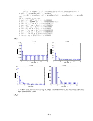
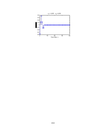
419. Chapter 10 (2e)
10.1 For an input x1[n] and x2[n], the outputs of the factor-of-L up-sampler are, respectively, given
by
xu1[n] =
x1[n/ L], n = 0,± L,± 2L,K
0, otherwise,



and xu2[n]=
x2[n / L], n = 0, ± L, ± 2L,K
0, otherwise.



Let x2[n] = x1[n – no], where no is an integer. Then x2[n / L]= x1[(n / L) – no]. Hence,
xu2[n]=
x1[(n/ L) – no ], n = 0,± L,± 2L,K
0, otherwise.



But xu1[n – no] =
x1[(n – no )/ L], n – no = 0, ± L, ± 2L,K
0, otherwise,



Since xu2[n]≠ xu1[n– no],the up-
sampler is a time-varying system.
10.2 Consider first the up-sampler. Let x1[n] and x2[n] be the inputs with corresponding outputs
given by y1[n] and y2[n]. Now, y1[n] =
x1[n/ L], n = 0,± L,± 2L,K
0, otherwise,



and
y2[n] =
x2[n/ L], n = 0,± L,± 2L,K
0, otherwise.



Let us now apply the input x3[n] = αx1[n]+βx2[n],
with the corresponding output given by y3[n], where
y3[n] =
αx1[n / L]+ βx2[n/ L], n = 0,± L,± 2L,K
0, otherwise,



=
αx1[n/ L]
0



+
βx2[n / L] n = 0,± L,± 2L,K
0 otherwise,



= αy1[n]+ βy2[n]. Thus, the up-sampler is a
linear system.
Now, consider the down-sampler. Let x1[n] and x2[n] be the inputs with corresponding
outputs given by y1[n] and y2[n]. Now, y1[n] = x1[Mn], and y2[n] = x2[Mn]. Let us now apply
the input x3[n] = αx1[n]+βx2[n], with the corresponding output given by y3[n], where
y3[n] = x3[Mn]= αx1[Mn]+ βx2[Mn]. Thus, the down-sampler is a linear system.
10.3
From the figure, V(z) =
1
2
X(z1/ 2
)+
1
2
X(–z1/ 2
), W(z) =
z–1 /2
2
X(z1/ 2
)–
z–1/ 2
2
X(–z1/ 2
),
Vu(z) =
1
2
X(z) +
1
2
X(–z), Wu (z) =
z
–1
2
X(z) –
z
–1
2
X(–z). Hence,
Y(z) = z
–1
Vu (z) + Wu (z) = z
–1
X(z), or in other words, y[n] = x[n–1].
415

420. 10.4 c[n] =
1
M
WM
kn
k=0
M–1
∑ =
1
M
1– WM
nM
1– WM
n








. Hence, if n ≠ rM, c[n] =
1
M
1–1
1– WM
n








= 0. On the other
hand, if n = rM, then c[n] =
1
M
WM
kn
=
1
M
WM
krM
k=0
M–1
∑
k=0
M–1
∑ =
1
M
1
k=0
M–1
∑ = 1. Thus,
c[n] =
1, if n = rM,
0, otherwise.{
10.5
For the left-hand side figure, we have V1(z) = X(z
L
), Y1(z) =
1
M
X(zL / M
WM
kL
k =0
M–1
∑ ).
For the right-hand side figure,we have V2 (z) =
1
M
X(z1 / M
WM
k
)
k=0
M–1
∑ , Y2 (z) =
1
M
X(zL / M
WM
k
)
k=0
M–1
∑ .
Since L and M are relatively prime, WM
k
and WM
kL
take the same set of values for k = 0, 1, . ..,
M–1. Hence, Y1(z) = Y2(z).
10.6
For the left-hand side figure, we have V1(z) =
1
M
X(z1/ M
WM
k
)
k =0
M–1
∑ , Y1(z) =
1
M
H(z)X(z1/ M
WM
k
)
k =0
M–1
∑ ,
For the right-hand side figure,we have V2 (z) = H(z
M
)X(z), Y2 (z) =
1
M
H(zWM
kM
)X(z1/ M
WM
k
)
k=0
M–1
∑
=
1
M
H(z)X(z1/ M
WM
k
)
k=0
M–1
∑ . Hence, Y1(z) = Y2(z).
For the left-hand side figure, we have V1(z) = X(z
L
), Y1(z) = H(z
L
)X(z
L
). For the right-hand
side figure,we have V2 (z) = H(z)X(z), Y2 (z) = H(z
L
)X(z
L
). Hence, Y1(z) = Y2(z).
10.7
x[n] y[n]5 10 2 ≡
x[n] y[n]5 25 2 ≡ x[n] y[n]2 2
x1[n]
416

421. Hence, x1[n] = x[2n] and y[n] =
x1[n / 2], for n = 2r,
0, otherwise



=
x[n], for n = 2r,
0, otherwise



Therefore,
y[n] =
x[n], for n = 2r,
0, otherwise.



10.8
x[n] 3 3
w[n] u[n]
H0 (z)
H1(z)
H2 (z)
y0[n]
y1[n]
y2[n]
10.9 As outlined in Section 6.3, the transpose of a digital filter structure is obtained by reversing all
paths, replacing the pick-off node with an adder and vice-versa, and interchanging the input
and the output nodes. Moreover, in a multirate structure, the transpose of a factor-of-M down-
sampler is a factor-of-M up-sampler and vice-versa. Applying these operations to the factor-
of-M decimator shown on the left-hand side, we arrive at a factor-of-M interpolator as indicated
on the right-hand side in the figure below.
10.10 Applying the transpose operation to the M-channel analysis filter bank shown below on the
left-hand side, we arrive at the M-channel synthesis filter bank shown below on the right-hand
side.
417

422. x[n] H0 (z)
H1(z)
v0[n]
v1[n ]
vM−1[n]HM−1(z)
M
M
M
≡
y[n] H0 (z)
H1(z)
v 0[n]
v1[n]
v M−1[n]HM−1(z)
M
M
M
≡
y[n]H0 (z)
H1(z)
v0[n]
v1[n]
vM−1[n] HM−1(z)
M
M
M
10.11 Specifications for H(z) are as follows:
Fp = 180 Hz, Fs = 200 Hz, δp = 0.002, δs = 0.001.
H(z) 30
12 kHz 12 kHz 400 Hz
We realize H(z) as H(z) = G(z6
)F(z).
12 kHz 12 kHz 400 Hz2 kHz12 kHz
56F(z) G(z6
)
Therefore, specifications for G(z) are as follows:
Fp = 1080 Hz, Fs = 1200 Hz, δp = 0.001, δs = 0.001. Here, ∆f =
120
12000
. Hence, from
Eq. (7.15), order of G(z) is given by NG =
–20log10 0.001× 0.001 –13
14.6(120 /12000)
=
47×12000
14.6 ×120
= 321.92.
Likewise, specifications for F(z) are : Fp = 180 Hz, Fs = 1800 Hz, δp = 0.001, δs = 0.001.
Here, ∆f =
1620
12000
. Hence, order of F(z) is given by
NF =
–20 log10 10–6 –13
14.6(1620/ 12000)
=
47 ×12000
14.6×1620
= 23.846. Thus, we choose NG = 322 and NF = 24 .
RM,G = (322 +1)×
2000
5
= 129,200 muliplications/second (mps), and
RM,F = (24 +1) ×
12000
6
= 50,000 mps
418

423. Hence, total no. of mps = 179,200. Hence the computational complexity of this particular IFIR
implementation is slightly higher here than that in Example 10.8.
12 kHz 12 kHz 400 Hz
6 5G(z)
2 kHz 2 kHz
F(z)
10.12 We realize H(z) as H(z) = G(z5
)F(z).
12 kHz 12 kHz 400 Hz12 kHz
5 6F(z) G(z
5
)
2.4 kHz
Specifications for G(z) are: Fp = 900 Hz, Fs = 1000 Hz, δp = 0.001, δs = 0.001. Here,
∆f =
100
12000
. Hence, from Eq. (7.15), order of G(z) is given by
NG =
–20log10 0.001× 0.001 –13
14.6(100 /12000)
=
47×12000
14.6 ×100
= 386.3. Likewise, specifications for F(z)
are : Fp = 180 Hz, Fs = 2200 Hz, δp = 0.001, δs = 0.001. Here, ∆f =
2020
12000
. Hence, order of
F(z) is given by NF =
–20 log10 10–6 –13
14.6(2020 /12000)
=
47×12000
14.6× 2020
= 19.124. Thus, we choose NG = 387
and NF = 20 .
G(z)
12 kHz 12 kHz 400 Hz
5 6F(z)
2.4 kHz 2.4 kHz
RM,G = (387 +1)×
2400
6
=155,200 muliplications/second (mps), and
RM,F = (20 +1)×
12000
5
= 50, 400 mps
Hence, total no. of mps = 205,600. Hence the computational complexity of this particular IFIR
implementation is slightly higher here than that in Example 10.8 and in Problem 10.11.
10.13
H(z) 20
60 kHz 60 kHz 3 kHz
Specifications for H(z) are: Fp = 1250 kHz, Fs =1500 kHz, δp = 0.02 and δs = 0.01. Hence,
from Eq. (7.15), order N of H(z) is given by
N =
–20log10 0.02 × 0.01 –13
14.6(250/ 60000)
=
23.989× 60000
14.6 × 250
= 394.34 . We thus choose N = 395.
Computational complexity is therefore = 396 ×
60,000
20
= 1,188,000.
419

424. 10.14 Original decimation filter H(z) specifications: Fp = 1250 Hz, Fs =1500 , δp = 0.02, δs = 0.01.
The 4 possible IFIR implementations of H(z) are as follows: (A) H(z) = G(z5
)F(z),
(B) H(z) = G(z4
)F(z), (C) H(z) = G(z2
)F(z),and (D) H(z) = G(z10
)F(z).
Case A: Specfications for G(z): Fp = 1250 × 5 = 6250 Hz, Fs =1500 × 5 = 7500 Hz,
δp = 0.01, δs = 0.01. Here ∆f =
1250
60,000
. Hence, using Eq. (10.26), we obtain the order of G(z)
as NG =
−20 log10 0.01 × 0.01 −13
14.6(1250 / 60000)
= 88.767.
Specfications for F(z): Fp = 1250 Hz, Fs =
60000 − 5× 1500
5
=10,500 Hz,
δp = 0.01, δs = 0.01. Here ∆f =
9250
60,000
. Hence, using Eq. (10.26), we obtain the order of F(z)
as NF =
−20log10 0.01 × 0.01 − 13
14.6(9250 / 60000)
= 11.996. We thus choose NG = 89 and NF = 12.
Hence, RM,G = (89 + 1) ×
12000
4
= 270,000 mps and RM,F = (12 + 1) ×
60000
5
=156,000 mps.
Hence, total computational complexity = 426,000 mps.
Case B: Specfications for G(z): Fp = 1250 × 4 = 5000 Hz, Fs =1500 × 4 = 9000 Hz,
δp = 0.01, δs = 0.01. Here ∆f =
1000
60,000
. Hence, using Eq. (10.26), we obtain the order of G(z)
NG =
−20 log10 0.01 × 0.01 −13
14.6(1000 / 60000)
= 110.96
Specfications for F(z): Fp = 1250 Hz, Fs =
60000 − 5× 1500
5
=10,500 Hz,
δp = 0.01, δs = 0.01. Here ∆f =
12250
60,000
. Hence, using Eq. (10.26), we obtain the order of F(z)
NF =
−20log10 0.01 × 0.01 − 13
14.6(12250 / 60000)
= 0.0579 . We thus choose NG = 111 and NF = 10.
Hence, RM,G = (111+ 1) ×
15000
5
= 336,000 mps and RM,F = (10 + 1) ×
60000
4
=165,000 mps.
Hence, total computational complexity = 501,000 mps.
Case C: Specfications for G(z): Fp = 1250 × 2 = 2500 Hz, Fs =1500 × 2 = 3000 Hz,
δp = 0.01, δs = 0.01. Here ∆f =
500
60,000
. Hence, using Eq. (10.26), we obtain the order of G(z)
NG =
−20 log10 0.01 × 0.01 −13
14.6(500 / 60000)
= 221.92 .
420

425. Specfications for F(z): Fp = 1250 Hz, Fs =
60000 − 2 ×1500
2
= 28,500 Hz,
δp = 0.01, δs = 0.01. Here ∆f =
12250
60,000
. Hence, using Eq. (10.26), we obtain the order of F(z)
NF =
−20log10 0.01 × 0.01 − 13
14.6(27250 / 60000)
= 4.0179 . We thus choose NG = 222 and NF = 5.
Hence, RM,G = (222 + 1) ×
30000
10
= 669,000 mps and RM,F = (5+ 1) ×
60000
2
= 180,000 mps.
Hence, total computational complexity = 849,000 mps.
Case D: Specfications for G(z): Fp = 1250 × 10 =12500 Hz, Fs =1500 ×10 = 15000 Hz,
δp = 0.01, δs = 0.01. Here ∆f =
2500
60,000
. Hence, using Eq. (10.26), we obtain the order of G(z)
NG =
−20 log10 0.01 × 0.01 −13
14.6(2500 / 60000)
= 44.384.
Specfications for F(z): Fp = 1250 Hz, Fs =
60000 − 10 × 1500
10
= 4,500 Hz,
δp = 0.01, δs = 0.01. Here ∆f =
3250
60,000
. Hence, using Eq. (10.26), we obtain the order of F(z)
NF =
−20log10 0.01 × 0.01 − 13
14.6(3250 / 60000)
= 34.141. We thus choose NG = 45 and NF = 35.
Hence, RM,G = (45 + 1) ×
6000
2
=138,000 mps and RM,F = (35 +1) ×
60000
10
= 216,000 mps.
Hence, total computational complexity = 354,000 mps.
Thus, Case D has the lowest computational complexity.
10.15 (a) Specifications for H(z) are: Fp = 200 Hz, Fs = 300 Hz, δp = 0.002 and δs = 0.004.
15 H(z)
600 Hz 9 kHz 9 kHz
Here, ∆f =
100
9000
. Hence, from Eq. (10.26), order N of H(z) is given by
N =
–20log10 0.002× 0.004 –13
14.6(100 / 9000)
=
37.969× 9000
14.6× 100
= 234.06. We choose N = 235. Hence,
computational complexity = (235+1)×
9000
15
= 141,600 mps.
(b) We realize H(z) = G(z5
)F(z).
600 Hz 9 kHz9 kHz
3 5G(z) F(z)
1.8 kHz 1.8 kHz
421

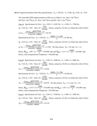
426. Specifications for G(z) are: Fp = 200 Hz, Fs = 300 Hz, δp = 0.002 and δs = 0.004. Here,
∆f =
100
9000
. Hence, from Eq. (7.15), order N of H(z) is given by
10.16 (a) H1(z) =
p0 + p1z–1
1+ d1
z–1 . H1(zW2
1
) = H1(−z) =
p0 − p1z–1
1− d1
z–1 . Thus,
E0(z2
) =
1
2
H1(z)+ H1(−z)[ ]=
1
2
p0 + p1z–1
1+ d1
z–1 +
p0 − p1z–1
1− d1
z–1








=
p0 − p1d1z−2
1− d1
2z−2 , and
z–1
E1(z2
) =
1
2
H1(z)− H1(−z)[ ]=
1
2
p0 + p1z–1
1+ d1
z–1 −
p0 − p1z–1
1− d1
z–1








=
(p1 − p0d1)z−1
1− d1
2z−2 . Hence, a two-
band polyphase decomposition of H1(z) is given by
H1(z) =
p0 − p1d1z−2
1− d1
2z−2








+ z−1 p1 − p0d1
1− d1
2z−2








.
(b) H2(z) =
2+ 3.1z–1
+1.5z–2
1+ 0.9z–1 + 0.8z–2 . H2(zW2
1
) = H2 (−z) =
2− 3.1z–1
+ 1.5z–2
1− 0.9z–1 + 0.8z–2 . Thus,
E0(z2
) =
1
2
H2(z) + H2 (−z)[ ]=
1
2
2 + 3.1z–1
+ 1.5z–2
1+ 0.9z–1 + 0.8z–2 +
2 − 3.1z–1
+ 1.5z–2
1− 0.9z–1 + 0.8z–2








=
4+ 0.62z–2
+ 2.4z–4
1+ 0.79 z–2 + 0.64z–4 .
z−1
E1(z2
) =
1
2
H2 (z) − H2(−z)[ ]=
1
2
2 + 3.1z–1
+ 1.5z–2
1+ 0.9z–1 + 0.8z–2 −
2 − 3.1z–1
+ 1.5z–2
1− 0.9z–1 + 0.8z–2








=
2.6z–1
+ 2.26z–3
1+ 0.79 z–2 + 0.64z–4 . Hence, a two-band polyphase decomposition of H2(z) is given by
H2(z) =
4 + 0.62 z–2
+ 2.4z–4
1+ 0.79z–2 + 0.64 z–4





 + z−1 2.6+ 2.26 z–2
1+ 0.79 z–2 + 0.64z–4





 .
(c) H3(z) =
2 + 3.1z–1
+1.5z–2
+ 4z–3
(1– 0.5z–1)(1+ 0.9z–1 + 0.8z–2)
=
2+ 3.1z–1
+1.5z–2
+ 4z–3
1+ 0.4z–1 + 0.35z–2 − 0.4z–3 .
H3(−z) =
2 − 3.1z–1
+ 1.5z–2
− 4z–3
1− 0.4z–1 + 0.35z–2 + 0.4z–3 .
E0(z2
) =
1
2
H3(z)+ H3(−z)[ ]=
1
2
2 + 3.1z–1
+1.5z–2
+ 4z–3
1+ 0.4z–1 + 0.35z–2 − 0.4z–3 +
2− 3.1z–1
+1.5z–2
− 4z–3
1− 0.4z–1 + 0.35z–2 + 0.4z–3








=
4 +1.92 z–2
+ 0.33z–4
+3.2z–6
1+ 0.54 z–2 + 0.4425z–4 − 0.16z–6 .
422

427. z−1
E1(z2
) =
1
2
H3(z)− H3(−z)[ ]=
1
2
2 + 3.1z–1
+1.5z–2
+ 4z–3
1+ 0.4z–1 + 0.35z–2 − 0.4z–3 −
2− 3.1z–1
+1.5z–2
− 4z–3
1− 0.4z–1 + 0.35z–2 + 0.4z–3








=
4.6z–1
+10.57z–3
+ 4z–5
1+ 0.54 z–2 + 0.4425z–4 − 0.16z–6 . Hence, a two-band polyphase decomposition of H3(z) is
given by H3(z) =
4 +1.92 z–2
+ 0.33z–4
+3.2z–6
1+ 0.54 z–2 + 0.4425z–4 − 0.16 z–6





 + z−1 4.6+10.57z–2
+ 4z–4
1+ 0.54z–2 + 0.4425z–4 − 0.16z–6






10.17 (a) H1(z) =
p0 + p1z–1
1+ d1
z–1 = z−k
k =0
2
∑ Ek(z3
). Thus,
H1
(z)
H1(W3
1
z)
H1(W3
2z)












=
1 1 1
1 W3
−1
W3
−2
1 W3
−2 W3
−4












E0
(z3)
z−1
E1(z3
)
z−2
E2(z3
)












=
1 1 1
1 W3
−1
W3
−2
1 W3
−2 W3
−1












E0
(z3 )
z−1
E1(z3
)
z−2
E2(z3
)












or
E0
(z3 )
z−1
E1(z3
)
z−2
E2(z3
)












=
1 1 1
1 W3
−1
W3
−2
1 W3
−2 W3
−1












−1
H1
(z)
H1(W3
1
z)
H1(W3
2z)












=
1
3
1 1 1
1 W3
1
W3
2
1 W3
2 W3
1












H1
(z)
H1(W3
1
z)
H1(W3
2z)












. Theefore,
E0(z3
) =
1
3
H1(z)+ H1(zW3
1
) + H1(z W3
2
)[ ]
=
1
3
p0 + p1z−1
1+ d1
z−1 +
p0 + p1ej2π /3z−1
1+ d1
ej2π/ 3z−1 +
p0 + p1ej4π/ 3z−1
1+ d1
ej4π/ 3z−1








=
p0 + p1d1
2z−3
1+ d1
3z−3 .
z−1
E1(z3
) =
1
3
H1(z)+ W3
1
H1(z W3
1
) + W3
2
H1(z W3
2
)[ ]
=
1
3
p0 + p1z−1
1+ d1
z−1 + ej2π / 3 p0 + p1ej2π /3z−1
1+ d1
ej2π /3z−1 + ej4π/ 3 p0 + p1ej4π/ 3z−1
1+ d1
ej4π/ 3z−1








= z−1 p1 − p0d1
1+ d1
3z−3 .
z−2
E2 (z3
) =
1
3
H1(z)+ W3
2
H1(z W3
1
)+ W3
1
H1(z W3
2
)[ ]
=
1
3
p0 + p1z−1
1+ d1
z−1 + ej4π/ 3 p0 + p1ej2π / 3z−1
1+ d1
ej2π / 3z−1 + ej2π/ 3 p0 + p1ej4π/ 3z−1
1+ d1
ej4π/ 3z−1








= z−2 −p1d1 + p0d1
2
1+ d1
3z−3 .
Hence, E0(z) =
p0 + p1d1
2z−1
1+ d1
3z−1 , E1(z) =
p1 − p0d1
1+ d1
3z−1 , and E2(z) =
−p1d1 + p0d1
2
1+ d1
3z−1 .
(b) H2(z) =
2+ 3.1z–1
+1.5z–2
1+ 0.9z–1 + 0.8z–2 .
H2
(z)
H2(W3
1
z)
H2 (W3
2z)












=
1 1 1
1 W3
−1
W3
−2
1 W3
−2 W3
−1












E0
(z3)
z−1
E1(z3
)
z−2
E2 (z3
)












or
E0
(z3 )
z−1
E1(z3
)
z−2
E2(z3
)












=
1
3
1 1 1
1 W3
1
W3
2
1 W3
2 W3
1












H2
(z)
H2(W3
1
z)
H2(W3
2z)












.
423

428. Thus, E0(z3
) =
1
3
H2(z) + H2 (z W3
1
) + H2 (z W3
2
)[ ]
=
1
3
2+ 3.1z–1
+1.5z–2
1+ 0.9z–1 + 0.8z–2 +
2+ 3.1ej2π/ 3
z–1
+1.5ej4π /3
z–2
1+ 0.9ej2π/ 3z–1 + 0.8ej4π / 3 z–2 +
2 + 3.1ej4π / 3
z–1
+ 1.5ej2π/ 3
z–2
1+ 0.9ej4π/ 3z–1 + 0.8e j2π/ 3 z–2








=
6 − 8.277z–3
+ 2.88z–6
1−1.431z–3 + 0.512z–6 .
z−1
E1(z3
) =
1
3
H2(z) + W3
1
H2 (z W3
1
) + W3
2
H2 (zW3
2
)[ ]
=
1
3
[
2 + 3.1z–1
+1.5z–2
1+ 0.9z–1 + 0.8z–2 + ej2π /3 2 + 3.1ej2π /3
z–1
+1.5ej4π/ 3
z–2
1+ 0.9ej2π / 3z–1 + 0.8ej4π/ 3 z–2
+ ej4π/ 3 2 + 3.1ej4π/ 3
z–1
+1.5ej2π/ 3
z–2
1+ 0.9ej4π/ 3z–1 + 0.8ej2π/ 3 z–2 ]= z−1 3.9− 2.811z–3
1−1.431z–3 + 0.512z–6 .
z−2
E2 (z3
) =
1
3
H3(z)+ W3
2
H3(zW3
1
)+ W3
1
H3(z W3
2
)[ ]
=
1
3
[
2 + 3.1z–1
+1.5z–2
1+ 0.9z–1 + 0.8z–2 + ej4π / 3 2 + 3.1ej2π / 3
z–1
+1.5ej4π/ 3
z–2
1+ 0.9ej2π / 3z–1 + 0.8ej4π/ 3 z–2
+ ej2π / 3 2 + 3.1ej4π/ 3
z–1
+ 1.5e j2π/ 3
z–2
1+ 0.9ej4π/ 3z–1 + 0.8ej2π/ 3 z–2 ]= z−2 −3.81+ 2.712z–3
1−1.431z–3 + 0.512z–6 . Hence,
E0(z) =
6 −8.277z–1
+ 2.88z–2
1− 1.431z–1 + 0.512z–2 , E1(z) =
3.9− 2.811z–1
1−1.431z–1 + 0.512z–2 , and
E2(z) =
−3.81+ 2.712z–1
1−1.431z–1 + 0.512z–2 .
10.18 A computationally efficient realization of the factor-of-4 decimator
is obtained by applying a 4-branch polyphase decomposition to H(z):
H(z) = E0 (z
4
) + z
–1
E1(z
4
)+ z
–2
E2(z
4
) + z
–3
E3(z
4
).
and then moving the down-sampler through the polyphase filters resulting in
E0 (z)
E1(z)
E2 (z)
E3 (z)
z−1
z−1
z−1
4
4
4
4
w1[n]
w2[n]
w3[n]
w4[n]
y[n]
424

429. Further reduction in computational complexity is achieved by sharing comon multipliers if
H(z) is a linear-phase FIR filter. For example, for a length-16 Type I FIR transfer function
H(z) = h[0]+ h[1]z
–1
+ h[2]z
–2
+ h[3]z
–3
+ h[4]z
–4
+ h[5]z
–5
+ h[6]z
–6
+ h[7]z
–7
+ h[7]z
–8
+h[6]z
–9
+ h[5]z
–10
+ h[4]z
–11
+ h[3]z
–12
+ h[2]z
–13
+ h[1]z
–14
+ h[0]z
–15
,
for which E0(z) = h[0]+ h[4]z
–1
+ h[7]z
–2
+ h[3]z
–3
, E1(z) = h[1]+ h[5]z
–1
+ h[6]z
–2
+ h[2]z
–3
,
E2(z) = h[2]+ h[6]z
–1
+ h[5]z
–2
+ h[1]z
–3
, and E3(z) = h[3]+ h[7]z
–1
+ h[4]z
–2
+ h[0]z
–3
.
From the above figure it follows that Y(z) = E0 (z)W1(z)+ E1(z)W2 (z) + E2 (z)W3(z)+ E3(z)W4 (z)
= h[0] W1(z) + z
−3
W4(z)( )+ h[4] z
−1
W1(z)+ z
−2
W4(z)( )
+h[7] z
−2
W1(z)+ z
−1
W4 (z)( )+ h[3] z
−3
W1(z)+ W4 (z)( )
+ h[1] W2 (z)+ z
−3
W3(z)( )+ h[5] z
−1
W2 (z) + z
−2
W3(z)( )
+h[6] z
−2
W2 (z) + z
−1
W3(z)( )+ h[2] z
−3
W2 (z)+ W3(z)( ).
A computationally efficient factor-of-4 decimator structure based on the above equation is then
as shown below:
z
−1
z
−1
z
−1
z
−1
z
−1
z
−1
z
−1
z
−1
z
−1
z
−1
z
−1
z
−1
z
−1 z
−1
z
−1
y[n]
w1[ n]
w4[n]
w2[n]
w3[n]
x[n] 4
4
4
4
h[0]
h[4]
h[7]
h[1]
h[5]
h[6]
h[2]
h[3]
10.19 A computationally efficient realization of the factor-of-3 interpolator is obtained by applying
a 3-branch Type II polyphase decomposition to the interpolation filter H(z):
H(z) = R2(z3
) + z–1
R1(z3
)+ z–2
R0(z3
),
and then moving the up-sampler through the polyphase filters resulting in
425

430. z−1
z−1
3
3
3
R0(z)
R1(z)
R2(z)
x[n]
w1[n]
w2[n]
w3[n]
From the above figure it follows that
W3(z) = h[0]X(z) + h[3]z−1
X(z)+ h[6]z−2
X(z) + h[5]z−3
X(z) + h[2]z−4
X(z),
W1(z) = h[2]X(z) + h[5]z−1
X(z)+ h[6]z−2
X(z) + h[3]z−3
X(z) + h[0]z−4
X(z), and
W2(z) = h[1] X(z) +z−4
X(z)( )+ h[4] z−1
X(z)+ z−3
X(z)( )+ h[7]z−2
X(z).
A computationally efficient factor-of-3 interpolator structure based on the above equations is
then as shown below:
x[n]
z−1
z−1
z−1
z−1 y[n]
h[0]
h[4]
h[7]
h[1]
h[5] h[6]h[2] h[3]
z−1
z−1
z−1
z−1
z−1 z−1
z−1
z−1
3
3
3
z−1
z−1
w1[n]
w2[n]
w3[n]
10.20 H(z) = z−i
i=0
N−1
∑ = (1+ z−1
)+ (z−2
+ z−3
)+L+ (z−(N−2)
+ z−(N−1)
)
= (1+ z−1
) 1+ z−2
+ z−4
+L+ z−(N−2)
( )= (1+ z−1
)G(z2
) where G(z) = z−2i
i=0
(N / 2)−1
∑ . Using a
similar technique we can show that G(z) = (1+ z−1
) z−2i
i=0
(N / 4)−1
∑







 . Therefore we can write
H(z) = (1+ z−1
)(1+ z−2
) z−2i
i=0
(N / 4)−1
∑







 = (1+ z−1
)(1+ z−2
)F(z4
) where F(z) = z−i
i=0
(N / 4)−1
∑ . Continuing
426

431. this decomposition process further we arrive at H(z) = (1+ z−1
)(1+ z−2
)L(1+ z−2K −1
), where
N = 2K
. Realization of a factor-of-16 decimator using a box-car decimation filter is as
indicated below:
x[n] y[n]16
16
16
16
z
–1
z
–1
z
–1
z
–1
10.21 Let u[n] denote the output of the factor-of-L interpolator. Then,
E =
u[n] − u[n − 1]( )2
n=−∞
∞
∑
u2
[n]
n =−∞
∞
∑
(1)
and C =
u[n]u[n − 1]
n=−∞
∞
∑
u2
[n]
n =−∞
∞
∑
. (2)
Substituting Eq. (2) in Eq. (1) we get E = 2(1− C). Hence, as C →1, i.e., as the signal u[n]
becomes highly correlated, E → 0.
Now, by Parseval's relation, u[n]v[n]
n =−∞
∞
∑ =
1
2π
U(ejω
)V *(ejω
)
−π
π
∫ dω, where U(e jω
) and
V(ejω
) are the DTFTs of u[n] and v[n], respectively. If we let v[n] = u[n–1] in the numerator
of Eq. (1) and v[n] = u[n] in the denominator of Eq. (1), then we can write
E =
1
2π
U(ejω
)
2
e jω
dω
−π
π
∫
1
2π
U(ejω
)
2
dω
−π
π
∫
=
U(ejω
)
2
cos(ω)dω
0
π
∫
U(ejω
)
2
dω
0
π
∫
,
assuming u[n] to be a real sequence. If x[n] is assumed to be a broadband signal with a flat
magnitude spectrum, i.e., X(ejω
) =1 for 0 ≤ ω ≤ π, then the magnitude spectrum of u[n] is
427

432. bandlimited to the range 0 ≤ ω ≤ π / L, i.e., U(ejω
) =
1, for 0 ≤ ω < π / L,
0, otherwise.



Therefore,
C =
cos(ω)dω
0
π/L
∫
dω
0
π/ L
∫
=
sin(π / L)
(π / L)
. Hence, as L → ∞, C →1.
10.22 Analysis of the structure of Figure P10.4 yields
W(ejω
) = X(ejω/ M
), R(ejω
) = H(ejω
)X(ejω/ M
),
S(ejω
) = e−jωL
R(ejω
) = e− jωL
H(e jω
)X(ejω/ M
), Y(ejω
) =
1
M
S(e−jωk / M
k=0
M−1
∑ ejω/ M
).
If the lowpass filter is assumed to be close to an ideal lowpass filter with a cutoff at ω / M, we
can assume that all images of X(e jω
) are suppressed leaving only the k = 0 term in the
expression for Y(ejω
). Hence, we can write
Y(ejω
) ≅
1
M
S(ejω/ M
) ≅
1
M
H(ejω/M
)e−jωL/ M
X(ejω
).
Since H(z) is a Type 1 FIR filter with exact linear phase and a delay of (N −1) / 2 = KM
samples and a magnitude response equal to M in the passband, we have
Y(ejω
) =e−jωK
e− jωL /M
X(ejω
).
Thus, the structure of Figure P10.4 is approximately an allpass filter with a fixed delay of K
samples and a variable noninteger delay of L/M samples.
10.23 An ideal M-th band lowpass filter H(z) is characterized by a frequency response
H(ejω
) =
1, –
π
M
≤ ω ≤
π
M
,
0, otherwise.




H(z) can be expressed in an M-branch polyphase form as: H(z) = z
−k
Hk (z
M
k=0
M−1
∑ ).
From above H(zWM
r
r=0
M−1
∑ ) = MH0(z
M
). Therefore, H0(ejωM
) =
1
M
H(ej(ω−2πr / M)
)
r=0
M−1
∑ =
1
M
. Or
in other words, H0(z
M
) is an allpass function.
Similarly for the remaining subfilters.
10.24 An equivalent realization of the structure of Figure 10.34 obtained by realizing the filter H(z)
in a Type I polyphase form is as shown below on the left. By moving the down-sampler
through the system and invoking the cascade equivalence #1 of Figure 10.14 we arrive at the
structure shown below on the right.
428

433. z
−1
z−1
z
−1
EL–1(z
L
)
L L
E1(z
L
)
E0
(zL
)
E2(z
L
)
≡
z−1
z−1
z
−1
E0(z)
E1(z)
E2(z)
EL–1(z)
L L
L
L
L
which reduces to the structure shown below on the left from which we arrive at the simplified
equivalent structure shown below on the right.
E0(z)L L ≡ E0(z)
10.25 (a) H(z) = h[n]z
−n
n=0
N−1
∑ .
Let H0(z
2
) =
1
2
h[2i]+ h[2i + 1]( )z
−2i
i=0
N
2
−1
∑ , and H1(z
2
) =
1
2
h[2i]− h[2i +1]( )z
−2i
i=0
N
2
−1
∑ . Then
(1+ z
−1
)H0 (z
2
) + (1− z
−1
)H1(z
2
) = h[2i]z
−2i
+ h[2i +1]z
−2i+1
i=0
N
2
−1
∑
i=0
N
2
−1
∑ = H(z).
(b) H(z) = (1+ z
−1
)H0 (z
2
)+ (1− z
−1
)H1(z
2
)
= H0(z
2
) + H1(z
2
)( )+ z
−1
H0(z
2
)− H1(z
2
)( )= E0 (z
2
) + z
−1
E1(z
2
). Therefore,
E0(z) = H0 (z) + H1(z), and E1(z) = H0(z)− H1(z).
(c) Now H(z) = 1 z
−1
[ ]1 1
1 −1




H0(z
2
)
H1(z2
)








= 1 z
−1
[ ]
H0
(z2
) + H1
(z2
)
H0 (z
2
) − H1(z
2
)








= H0(z
2
) + H1(z
2
)( )+ z
−1
H0(z
2
)− H1(z
2
)( ) = (1+ z
−1
)H0(z
2
) +(1− z
−1
)H1(z
2
).
(d) If L = 2, i.e. N = 22, then we can express H0(z
2
) = (1+ z
−2
)H00(z
4
) +(1− z
−2
)H01(z
4
),and
H1(z
2
) = (1+ z
−2
)H10(z
4
)+ (1− z
−2
)H11(z
4
). Substituting these expressions in
H(z) = (1+ z
−1
)H0 (z
2
)+ (1− z
−1
)H1(z
2
) we get
H(z) = (1+ z
−1
) (1+ z
−2
)H00(z
4
) + (1− z
−2
)H01(z
4
)[ ]+ (1− z
−1
) (1+ z
−2
)H10(z
4
) +(1− z
−2
)H11(z
4
)[ ]
= (1+ z
−1
)(1+ z
−2
)H00(z
4
) + (1+ z
−1
)(1− z
−2
)H01(z
4
)
429

434. +(1− z
−1
)(1+ z
−2
)H10(z
4
) +(1− z
−1
)(1− z
−2
)H11(z
4
)
= 1 z
−1
z
−2
z
−3
[ ]
1 1 1 1
1 −1 1 −1
1 1 −1 −1
1 −1 −1 1










H00(z4
)
H01(z
4
)
H10(z4
)
H11(z
4
)
















= 1 z
−1
z
−2
z
−3
[ ]R4
ˆH0 (z4
)
ˆH1(z
4
)
ˆH2 (z
4
)
ˆH3
(z4
)
















.
Continuing this process it is easy to establish that for N = 2L, we have
H(z) = 1 z
−1
L z
−(L −1)
[ ]RL
ˆH0(z
L
)
ˆH1
(zL
)
M
ˆHL −1(z
L
)














.
10.26 Now H(z) = 1 z
−1
z
−2
z
−3
[ ]R4
ˆH0(z4
)
ˆH1(z
4
)
ˆH2(z
4
)
ˆH3
(z4
)
















= 1 z
−1
z
−2
z
−3
[ ]
E0(z4
)
E1(z
4
)
E2(z
4
)
E3
(z4
)
















.
Therefore,
ˆH0 (z)
ˆH1(z)
ˆH2 (z)
ˆH3
(z)
















= R4
−1
E0
(z)
E1(z)
E2 (z)
E3(z)












=
1
4
R4
E0
(z)
E1(z)
E2(z)
E3(z)












=
1
4
1 1 1 1
1 −1 1 −1
1 1 −1 −1
1 −1 −1 1










E0
(z)
E1(z)
E2(z)
E3(z)












.
A length-16 Type 1 linear-phase FIR transfer function is of the form
H(z) = h0 + h1z
−1
+ h2z
−2
+ h3z
−3
+ h4z
−4
+ h5z
−5
+ h6z
−6
+ h7z
−7
+h7z
−8
+ h6z
−9
+ h5z
−10
+ h4z
−11
+ h3z
−12
+ h2z
−13
+ h1z
−14
+ h0z
−15
.
Hence, E0(z) = h0 + h4z
−1
+ h7z
−2
+ h3z
−3
, E1(z) = h1 + h5z
−1
+ h6z
−2
+ h2z
−3
,
E2(z) = h2 + h6z
−1
+ h5z
−2
+ h1z
−3
, E3(z) = h3 + h7z
−1
+ h4z
−2
+ h0z
−3
.
Thus, ˆH0(z) = g0 + g1z
−1
+ g1z
−2
+ g0z
−3
, ˆH1(z) = g2 + g3z
−1
− g3z
−2
− g2z
−3
,
ˆH2(z) = g4 + g5z
−1
− g4z
−2
− g5z
−3
, ˆH3(z) = g6 + g7z
−1
+ g7z
−2
+ g8z
−3
,
where g0 =
1
4
(h0 + h1 + h2 + h3), g1 =
1
4
(h4 + h5 + h6 + h7 ), g2 =
1
4
(h0 − h1 + h2 − h3),
g3 =
1
4
(h4 − h5 + h6 − h7 ), g4 =
1
4
(h0 + h1 − h2 − h3), g5 =
1
4
(h4 + h5 − h6 − h7 ),
g6 =
1
4
(h0 − h1 − h2 + h3 ), and g7 =
1
4
(h4 − h5 − h6 + h7). Observe that ˆH0(z) and
ˆH3(z) are Type 1 linear-phase FIR transfer functions, where as, ˆH1(z) and ˆH2(z) are Type 2
linear-phase FIR transfer functions. A computationally efficient realization of a factor-of-4
decimator using a four-band structural subband decomposition of the decimation filter H(z) is
developed below.
430

435. z−1
z−1
z
−1
4
4
4
4
ˆH0(z)
ˆH1(z)
ˆH2(z)
ˆH3(z)
4 × 4
Hadamard
matrix
R4
Because of the symmetric or antisymmetric impulse response, each subband filter ˆHi(z) can be
realized using only 2 multipliers. Hence, the final realization uses only 8 multipliers. Note also
that by delay-sharing, the total number of delays in implementing the four subband filters can
be reduced to 3.
10.27 y[n] = P−2(α)x[n − 2]+ P−1(α)x[n −1]+ P0(α)x[n]+ P1(α)x[n+ 1]+ P2(α)x[n + 2] where
P−2(α) =
(α +1)α(α −1)(α − 2)
(−2 +1)(−2)(−2−1)(−2− 2)
=
1
24
α4
− 2α3
− α2
+ 2α( ),
P−1(α) =
(α + 2)α(α −1)(α − 2)
(−1+ 2)(−1)(−1−1)(−1− 2)
= −
1
6
α4
− α3
− 4α2
+ 4α( ),
P0(α) =
(α + 2)(α + 1)(α −1)(α − 2)
(0 + 2)(0+ 1)(0−1)(0− 2)
=
1
4
α4
− 5α2
+ 4( ),
P1(α) =
(α + 2)(α +1)α(α − 2)
(1+ 2)(1+1)(1− 0)(1− 2)
= −
1
6
α4
+α3
− 4α2
− 4α( ),
P2(α) =
(α + 2)(α +1)α(α −1)
(2 + 2)(2+ 1)(2− 0)(2 −1)
=
1
24
α4
+ 2α3
− α2
− 2α( ).
We consider the computation of y[n], y[n+1], y[n+2], y[n+3] using 5 input samples: x[n-2]
through x[n+2].
For α0 = 0, P−2(α0 ) = 0, P−1(α0) = 0, P0(α0 ) = 1, P1(α0 ) = 0, and P2(α0 ) = 0.
For α1 = 5/ 4, P−2(α1) = −0.022, P−1(α1) = 0.127, P0(α1) = −0.3428, P1(α1) = 1.1426, and
P2(α1) = 0.0952.
For α2 =10 / 4, P−2(α2 ) = 0.2734, P−1(α2) = −1.4062, P0(α2 ) = 2.9531, P1(α2) = −3.2812, and
P2(α2 ) = 2.4609.
For α3 = 15/ 4, P−2(α3 ) = 3.5718, P−1(α3) = −17.2949, P0(α3 ) = 32.86, P1(α3) = −29.873, and
P2(α3) = 11.7358.
The block filter implementation is thus given by
431

436. y[n]
y[n+ 1]
y[n+ 2]
y[n + 3]










=
0 0 1 0 0
−0.022 0.127 −0.3428 1.1426 0.0952
0.2734 −1.4062 2.9531 −3.2812 2.4609
3.5718 −17.2949 32.86 −29.873 11.7358










x[n − 2]
x[n −1]
x[n]
x[n +1]
x[n + 2]












.
Another implementation is given by
y[n] = α4 1
24
x[n − 2]−
1
6
x[n− 1]+
1
4
x[n]−
1
6
x[n +1]+
1
24
x[n+ 2]( )
+ α3
−
1
12
x[n− 2]+
1
6
x[n −1]−
1
6
x[n+ 1]+
1
12
x[n + 2]( )
+ α2
−
1
24
x[n− 2]+
4
6
x[n −1]−
5
4
x[n]+
4
6
x[n +1]−
1
24
x[n+ 2]( )
+ α
1
12
x[n− 2]−
4
6
x[n −1]+
4
6
x[n +1]−
1
12
x[n + 2]( ) + x[n].
The Farrow structure implementation of the interpolator is shown below:
H0(z) H1(z) H2(z) H3(z)
α α α α
where H0(z) =
1
24
z−2
−
1
6
z−1
+
1
4
−
1
6
z +
1
24
z2
, H1(z) = −
1
12
z−2
+
1
6
z−1
+
1
6
z −
1
24
z2
,
H2(z) = −
1
24
z−2
+
4
6
z−1
−
5
4
+
4
6
z −
1
24
z2
, and H3(z) =
1
12
z−2
−
4
6
z−1
+
4
6
z −
1
12
z2
.
10.28 For a half-band zero-phase lowpass filter, the transfer function is of the form
H(z) = h[0] + z
−1
h[2n]
n=–∞
n≠0
∞
∑ z
−2n
, where h[0] =
1
2
. If the half-band filter has a zero at
z = –1, then H(−1) = h[0] − h[2n]
n= –∞
n≠0
∞
∑ = 0 or h[0] = h[2n]
n=–∞
n≠0
∞
∑ .
10.29 From Eq. (10.81), a zero-phase half-band filter H(z) satisfies the condition
H(z) + H(–z) = a constant.
(a) The zero-phase equivalent here is given by H1(z) = z + 2 + z
−1
. Hence,
H1(z) + H1(−1z) = z + 2 + z
−1
− z + 2 − z
−1
= 4. A plot of the magnitude response of H1(z)
is given below:
432

437. 0 0.2 0.4 0.6 0.8 1
0
0.2
0.4
0.6
0.8
1
ω /π
H1
(z)
(b) The zero-phase equivalent here is given by H2(z) = −z3
+ 9z +16 + 9z−1
− z−3
. Hence,
H2(z)+ H2(−z) = −z3
+ 9z +16 + 9z−1
− z−3
+ z3
− 9z + 16 − 9z−1
+z−3
= 32. A plot of the
magnitude response of H2(z) is given below:
0 0.2 0.4 0.6 0.8 1
0
0.2
0.4
0.6
0.8
1
ω /π
H2
(z)
(c) The zero-phase equivalent here is given by H3(z) = −3z3
+19 z + 32 +19z−1
− 3z−3
. Hence
H3(z) + H3(−z) = −3z3
+19z + 32 +19 z−1
− 3z−3
+ 3z3
−19z + 32 − 19z−1
+ 3z−3
= 64. A plot of
the magnitude response of H3(z) is given below:
0 0.2 0.4 0.6 0.8 1
0
0.2
0.4
0.6
0.8
1
ω /π
H3
(z)
(d) The zero-phase equivalent here is given by
H4(z) = 3z5
− 25z3
+150z + 256 +150z−1
− 25z−3
+ 3z−5
. Hence, H4(z) + H4 (−z) = 512. A plot
of the magnitude response of H4(z) is given below:
433

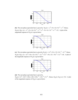
438. 0 0.2 0.4 0.6 0.8 1
0
0.2
0.4
0.6
0.8
1
ω/π
H
4
(z)
(e) The zero-phase equivalent here is given by
H5(z) = 9z5
− 44z3
+ 208z + 346 + 208z−1
− 44 z−3
+ 9z−5
. Hence H5(z)+ H5(−z) = 692. A plot
of the magnitude response of H5(z) is given below:
0 0.2 0.4 0.6 0.8 1
0
0.2
0.4
0.6
0.8
1
ω/π
H5
(z)
10.30 H0(z) =
Y0(z)
X(z)
= h[0]+ h[1]z
−1
+ h[2]z
−2
+ h[3]z
−3
+ h[4]z
−4
+ h[5]z
−5
+ h[6]z
−6
,
H1(z) =
Y1(z)
X(z)
= h[0]− h[1]z
−1
+ h[2]z
−2
− h[3]z
−3
+ h[4]z
−4
− h[5]z
−5
+ h[6]z
−6
.
z
−1 z
−1
z
−1
z
−1
z
−1
z
−1
h[0] h[1] h[2] h[3] h[4] h[5] h[6]
–1 –1 –1
x[n]
y0[n]
y1[n]
10.31 H0(z) =
Y0(z)
X(z)
= h[0]+ h[1]z
−1
+ h[2]z
−2
+ h[3]z
−3
+ h[4]z
−4
+ h[5]z
−5
+ h[6]z
−6
,
H1(z) =
Y1(z)
X(z)
= h[6]+ h[5]z
−1
+ h[4]z
−2
+ h[3]z
−3
+ h[2]z
−4
+ h[1]z
−5
+ h[0]z
−6
.
434

439. y1[n]
x[n]
y0[ n]
z
−1
z
−1 z
−1
z
−1 z
−1
z
−1
z
−1
z
−1 z
−1
z
−1 z
−1
z
−1
h[0]h[1]h[2]h[3]h[4]h[5]h[6]
10.31 (a)
H0
(z)
H1(z)
H2 (z)
H3(z)












=
1 1 1 1
1 −j −1 j
1 −1 1 −1
1 j −1 −j










E0
(z4)
z−1
E1(z4
)
z−2
E2(z4
)
z−3E3(z4)
















. Hence,
H0(z) = E0 (z4
) + z−1
E1(z4
) + z−2
E2(z4
)+ z−3
E3(z4
)
= 1+ 2z−1
+ 4z−2
+ z−3
+ 0.3z−4
− 1.5z−5
− 0.9z−6
+ 3.7z−7
− 0.8z−8
+ 3.1z−9
+ 2.3z−10
+1.7z−11
,
H1(z) = E0(z4
)− jz−1
E1(z4
) − z−2
E2(z4
) + jz−3
E3(z4
) = 1− j2z−1
− 4z−2
+ jz−3
+ 0.3z−4
+ j1.5z−5
− 0.9z−6
+ j3.7z−7
− 0.8z−8
− j3.1z−9
+ 2.3z−10
+ j1.7z−11
,
H2(z) = E0 (z4
) − z−1
E1(z4
)+ z−2
E2(z4
) −z−3
E3(z4
) =1− 2z−1
+ 4z−2
− z−3
+ 0.3z−4
+1.5z−5
− 0.9z−6
− 3.7z−7
− 0.8z−8
− 3.1z−9
+ 2.3z−10
−1.7z−11
,
H3(z) = E0(z4
)+ jz−1
E1(z4
) − z−2
E2(z4
) − jz−3
E3(z4
) = 1+ j2z−1
− 4z−2
− jz−3
+ 0.3z−4
− j1.5z−5
+ 0.9z−6
− j3.7z−7
+ 0.8z−8
+ j3.1z−9
− 2.3z−10
− j1.7z−11
(b)
H0 (ejω
)
1
0
ω
π
4
π
2
−
π
4
H1(e
jω
)
1
0 3π
4
π
ω
π
4
H3( ejω
)
1
0 5π
4
2ππ
ω
7π
4
435

440. 10.33 Y(z) = H0(z)G0(z)+ H1(z)G1(z)( )X(z). Now, H0(z) =
1+ z
−1
2
, and H1(z) =
1− z
−1
2
. Choose
G0(z) =
1+ z
−1
2
, and G1(z) = −
1− z
−1
2
. Then,
Y(z) =
1
4
(1+ z
−1
)
2
−
1
4
(1− z
−1
)
2




 X(z) =
1
4
(1+ 2z
−1
+ z
−2
−1+ 2z
−1
− z
−2
)X(z) = z
−1
X(z).
Or in other words, y[n] = x[n–1] indicating that the structure of Figure P10.7 is a perfect
reconstruction filter bank.
10.34 (a) Since H0(z) and H1(z) are power-complementary, H0(z)H0 (z
−1
)+ H1(z)H1(z
−1
) =1.
Now Y(z) = H0(z)G0(z)+ H1(z)G1(z)( )X(z) = z
−N
H0(z)H0(z
−1
)+ H1(z)H1(z
−1
)( )X(z)
= z
−N
X(z). Or in other words, y[n] = x[n–N] indicating that the structure of Figure P10.7 is a
perfect reconstruction filter bank.
(b) If H0(z) and H1(z) are causal FIR transfer functions of order N each, H0(z) and H1(z) are
polynomials in z–1. As a result, H0(z–1) and H1(z–1) are polynomials in z with the highest
power being zN. Hence, z–NH0(z–1) and z–NH1(z–1) are polynomials in z–1, making the
synthesis filters G0(z) and G1(z) causal FIR transfer functions of order N each.
(c) From Figure P10.7, for perfect reconstruction we require H0(z)G0(z) + H1(z)G1(z) = z–N
.
From part (a) we note that the PR condition is sdatisfied with G0(z) = z– N
H0(z–1
) and
G1(z) = z– N
H1(z–1
),if H0(z)H0 (z−1
)+ H1(z)H1(z−1
) =1, i.e. if H0(z) and H1(z) are power-
complementary. The last condition is satisfied if and only if H0(z) =
z−N /2
2
(z
−n0
+ z
n0
),
and H1(z) =
z−N / 2
2
(z
−n0
− z
n0
). As a result, G0(z) and G1(z) are also of the form
G0(z) =
z−N/ 2
2
(z
−n0
+ z
n0
), and G1(z) = –
z−N / 2
2
(z
−n0
− z
n0
).
10.35 From Eq. (10.97), Y(z) = T(z)X(z) + A(z)X(–z). Let Z–1{T(z)} = t[n], and Z–1{A(z)} =
a[n]. Then an inverse z-tranform of Eq. (10.97) then yields
y[n] = t[l ]x[n – l ]
l =–∞
∞
∑ + a[l ](−1)
n−l
x[n – l]
l =–∞
∞
∑ = t[l]+ (−1)
n−l
a[l ]( )x[n –l ]
l =– ∞
∞
∑ .
Define f0[n]= t[n]+ (−1)
−n
a[n], and f1[n] = t[n]− (−1)
−n
a[n]. Then we can write
y[n] =
f0[l ]x[n − l ],
l =–∞
∞
∑ for n even,
f1[l ]x[n − l ],
l =–∞
∞
∑ for n odd.





The corresponding equivalent realization of the 2-channel QMF bank is therefore as indicated
below:
436

441. x[n] y[n]
f1[n]
f0[n]
n even
n odd
As can be seen from the above representation, the QMF bank is, in general, a linear, time-
varying system with a period 2. Note that if A(z) = 0, then it becomes a linear, time-invariant
system.
10.36 (a) H0(z) =
1
4
A0(z2
) + z−1
A1(z2
){ }, and H1(z) =
1
4
A0 (z2
)− z−1
A1(z2
){ }. Hence,
E(z) =
A0
(z) A1
(z)
A0 (z) −A1(z)





, and R(z) =
A1(z) A1(z)
A0 (z) −A0(z)





.
(b) To prove E(z) is lossless, we need to show E† (ejω
)E(ejω
) = c2
I for some constant c:
E† (ejω
)E(ejω
) =
A0
*
(ejω
) A0
*
(ejω
)
A1(ejω) −A1(ejω )








A0
(ejω ) A1
(ejω)
A0 (ejω
) −A1(ejω
)








=
A0
(ejω )
2
+ A0
(ejω )
2
0
0 A1(ejω
)
2
+ A1(ejω
)
2










= 2I. Hence E(z) is lossless.
(c) R(z)E(z) =
1
4
2A1
(z)A0
(z) 0
0 2A1(z)A0 (z)





 =
A1(z)A0 (z)
2
I. Therefore,
R(z) =
A1(z)A0(z)
2
E-1(z).
(d) As in (c), R(z)E(z) =
A1(z)A0(z)
2
.
10.37 (a) G(z) =
1+ 3z
−1
+ 3z
−2
+ z
−3
6 + 2z
−2 =
1
2
1+ 3z
−2
3+ z
−2 +
3z
−1
+ z
−3
3+ z
−2







 =
1
2
1+ 3z
−2
3+ z
−2 + z
−1








=
1
2
A0 (z2
) + z−1
A1(z2
)( ), where A0(z) =
1+ 3z−1
3+ z−1 , and A1(z) = z−1
.
(b)
–1
z
−2
z
–1
1/2
1/3
437

442. (c) H(z) =
1
2
A0(z2
)− z−1
A1(z2
)( )=
1
2
1+ 3z−2
3+ z−2 − z−1





 =
1
2
1− 3z−1
+ 3z−2
− z−3
3+ z−2





 =
(1− z−1
)3
6+ 2z−2 .
(d)
10.38 Now the magnitude square function of an N-th order analog lowpass Butterworth transfer
function Ha(s) is given by Ha(jΩ)
2
=
1
1+ (Ω /Ωc
)2N , where Ωc is the 3-dB cutoff frequency.
For Ωc = 1, then Ha(jΩ)
2
=
1
1+ Ω2N . The corresponding transfer function of an N-th order
analog highpass transfer function is simply Ha
1
s( ), whose magnitude square function is given
by Ha
1
jΩ






2
=
Ω2N
1+ Ω2N . As a result, Ha(jΩ)
2
+ Ha
1
jΩ






2
=
1
1+ Ω2N +
Ω2N
1+ Ω2N = 1.
Now the bilinear transformation maps the analog frequency Ω to the digital frequency ω
through the relation ejω
=
1− jΩ
1+ jΩ
. As, –ejω
=
1−
1
jΩ
1+
1
jΩ
, the analog frequency 1/Ω is mapped to
the digital frequency π + ω . Hence the relation Ha(jΩ)
2
+ Ha
1
jΩ






2
=1, becomes
H0(ejω
)
2
+ H0( ej(π+ω)
)
2
= H0 (ejω
)
2
+ H0 (– ejω
)
2
= H0 (ejω
)
2
+ H1(ejω
)
2
= 1, where
H0(ejω
) is the frequency response of the digital lowpass filter H0(z) obtained by applying a
bilinear transformation to Ha(s) and H1(ejω
) is the frequency response of the digital highpass
filter H1(z) obtained by applying a bilinear transformation to Ha(1/s). Note that a transfer
function H0(z) satisfying the condition H0(ejω
)
2
+ H0(– ejω
)
2
=1, is called power-
symmetric.
Moreover, from the relation Ω = tan(ω / 2) it follows that the analog 3-dB cutoff frequency Ωc
= 1 is mapped into the digital 3-dB cutoff frequency ωc = π / 2. Hence, H(z) is a digital half-
band filter.
438

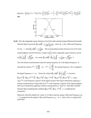
443. Let H0(z) =
P0(z)
D0 (z)
, where P0(z) and D0(z) are polynomials in z–1. Hence,
H0(ejω
) =
P0(ejω)
D0
(e jω )
. Now,
P0 (−ejω)P0
*(−ejω )
D0
(−ejω)D0
* (−e jω )
=
D0(ejω )D0
* (e jω )− P0(ejω)P0
*(ejω)
D0
(ejω)D0
* (ejω )
.
Note that there are no common factors between P0(ejω
) and D0(ejω
), and between P0
*
(ejω
)
and D0(ejω
). As a result there are no common factors between P0(−ejω
)P0
*
(−ejω
) and
D0(−ejω
)D0
*
(−e jω
). This implies then D0(ejω
)D0
*
(ejω
) = D0(−ejω
)D0
*
(−e jω
) As a result,
D0(ejω
)= D0 (−ejω
), or D0(ejω
)= d0(ej2ω
). Hence, D0(z) = d0(z2).
Since H0(z) =
P0(z)
D0 (z)
=
P0(z)
d0
(z2)
, it follows then H1(z) =
P0(−z)
d0
(z2)
. We have shown earlier that
H0(z) and H1(z) are power-complementary. Also P0(z) is a symmetric polynomial of odd
order and P0(–z) is an anti-symmetric polynomial of odd order. As a result we can express
H0(z) =
1
2
A0(z)+ A1(z)( ), and H1(z) =
1
2
A0 (z) − A1(z)( ). But H1(z) = H0(–z). Hence
H0(z) =
1
2
A0(−z) − A1(−z)( ). It therefore follows that A0(z) = A0 (−z) = A0(z2
), and
A1(z) = –A1(−z) = z−1
A1(z2
). Thus, H0(z) =
1
2
A0(z2
)+ z−1
A1(z2
)( ).
10.39 Ga(s) =
1
(s +1)(s2 + s +1)
. The corresponding digital transfer function H0(z) obtained by a
bilinear transformation is given by
H0(z) = Ga(s)
s=
z−1
z+1
=
(z +1)3
(z −1+ z +1) (z −1)2 + (z2 −1)+ (z +1)2
( )
=
(z +1)3
2z(3z2 +1)
=
(1+ z−1
)3
6 + 2z−2
=
1+ 3z−1
+ 3z−2
+ z−3
6+ 2z−2 =
1
2
1+ 3z−2
3+ z−2 + z−1








=
1
2
A0 (z2
)+ z−1
A1(2
)[ ] where A0 (z) =
1+ 3z−1
3+ z−1
and A1(z) =1.
The corresponding power-complementary transfer function is given by
H1(z) =
1
2
1+ 3z−2
3+ z−2 − z−1








=
(1− z−1
)3
6 + 2z−2 .
A realization of the QMF bank is as shown below:
439

444. 2
2
z
–1
z
–1
z
–1
–1
–1
1/ 3
10.40 Ga(s) =
1
s
5
+ 3.2361s
4
+ 5.2361s
3
+ 5.2361s
2
+ 3.2361s +1
. The corresponding digital transfer
function obtained by a bilinear transformation is given by
H0(z) = Ga(s)
s=
z−1
z+1
=
(1+ z
−1
)
5
18.9443 +12z
−2
+1.0557z
−4 =
0.0528(1+ z
−1
)
5
1+ 0.6334z
−2
+ 0.0557z
−4
=
0.0528 + 0.2639z
−1
+ 0.5279z
−2
+ 0.5279z
−3
+ 0.2639z
−4
+ 0.0528z
−5
1+ 0.6334z
−2
+ 0.0557z
−4
=
0.0528 + 0.5279z
−2
+ 0.2639z
−4
1+ 0.6334z
−2
+ 0.0557z
−4 +
0.2639z
−1
+ 0.5279z
−3
+ 0.0528z
−5
1+ 0.6334z
−2
+ 0.0557z
−4
=
0.0528(1+ 9.4704z−2
)
1+ 0.1056z−2 + z−1 0.2639(1+1.8948z−2
)
1+ 0.5278z−2
=
1
2
0.1056 + z−2
1+ 0.1056z−2 + z−1 0.5278+ z−2
1+ 0.5278z−2








=
1
2
A0 (z
2
)+ z
−1
A1(z
2
){ }, where
A0(z) =
0.1056 + z−1
1+ 0.1056z−1 , and A1(z) =
0.5278 + z−1
1+ 0.5278z−1 .
The corresponding power-complementary transfer function is given by
H1(z) =
1
2
A0(z2
) − z−1
A1(z2
){ }=
1
2
0.1056 + z−2
1+ 0.1056z−2 − z−1 0.5278+ z−2
1+ 0.5278z−2








.
In the realization of a magnitude-preserving QMF bank as shown in Figure 10.47, the
realization of the allpass filters A0(z) and A1(z) require 1 multiplier each, and hence the
realization of the analysis (and the synthesis) filter bank requires a total of 2 multipliers.
10.41 (a) Total number of multipliers required is 4(2N–1). Hence, total number of multiplications
per second is equal to 4(2N–1)FT = 4(2N–1)/T where FT = 1/T is the sampling frequency in
Hz.
(b) In Figure 10.47, H0(z) =
1
2
A0(z
2
) + z
−1
A1(z
2
){ }, and H1(z) =
1
2
A0 (z
2
)− z
−1
A1(z
2
){ }.
If order of A0 (z) is K and the order of A1(z) is L, then the order of H0(z) is 2K + 2L +1 = N.
Hence K+L = (N–1)/2. The total number of multpliers needed to implement A0 (z) is K while
the total number of multpliers needed to implement A1(z) is L. Hence the total number of
multipliers required to implement the structure of Figure 10.47 is 2(K+L) = N–1. However, the
440

445. multipliers here are operating at half of the sampling rate of the input x[n]. As a result, the
total number of multiplications per second in this case (N–1)FT/2 = (N–1)/2T.
10.42 H1(z) = z−N
H0(z−1
).
H0(z)
H1(z)
2
2
x[n] y0[n]
y1[n]
x[n]
y0[n]
y1[n]
2
2
h[N] h[N− 1] h[N− 2] h[1] h[0]
z
−1
z
−1
z
−1
z
−1
z
−1
z
−1
10.43 E(z) =
1 2 3 2
2 13 9 7
3 9 11 10
2 7 10 15










. For y[n] = 3x[n − 3], we require R(z)E(z) = 3I or
R(z) = 3E-1(z) = 3
1 2 3 2
2 13 9 7
3 9 11 10
2 7 10 15










−1
=
−3.8333 −1.5 4.8333 −2.333
−1.5833 0.25 0.5833 −0.333
4.5 0.5 −2.5 1.0
−1.75 −0.25 0.75 0










.
10.44 E(z) =
1 1 2
2 3 1
1 2 1








. For perfect reconstruction,
R(z) = E-1(z) =
1 1 2
2 3 1
1 2 1








−1
=
0.5 1.5 −2.5
−0.5 −0.5 1.5
0.5 −0.5 0.5








. A computationally efficient realization of
the filter bank is shown below:
z
−1
z
−1
z
−1
z
−1
3
3
3
3
3
3
(z)RE(z)
10.45 For perfect reconstruction we require
441

446. R(z) = E-1(z) =
1 2 3 4
3 2 1 5
2 1 4 3
4 2 3 1










−1
=
−0.4 0.2 0.16 0.12
0.7333 0.2 −0.76 0.3467
0.0667 0.2 0.24 0.0133
0.0667 0.2 0.16 −0.2133










. A computationally
efficient realization of the filter bank is shown below:
(z)RE(z)z
−1
z−1
z
−1
z−1
z
−1
z
−1
4
4
4
4
4
4
4
4
10.46 For perfect reconstruction we require
R(z) = E-1(z) =
4 2 3
5 4 1
2 1 3








−1
=
1.2222 −0.3333 −1.1111
−1.4444 0.6667 1.2222
−0.3333 0 0.6667








. A computationally
efficient realization of the filter bank is shown below:
z
−1
z
−1
z
−1
z
−1
3
3
3
3
3
3
(z)RE(z)
10.47 ˆX(z) = G0 (z) G1(z) L GL −1(z)[ ]
H0 (z) H0 (zW) L H0 (zW
L−1
)
H1
(z) H1
(zW) L H1
(zWL−1
)
M M O M
HL−1(z) HL−1(zW) L HL−1(zW
L−1
)














X(z)
X(zW)
M
X(zWL −1
)












.
To show the system of Figure 10.63 is, in general, periodic with a period L, we need to show
that if ˆX1(z) is the output for an input X1(z), and ˆX2(z) is the output for an input X2(z), then if
X2(z) = z
−L
X1(z),i.e. x2[n] = x1[n – L], then the corresponding output satisfies
ˆX2(z) = z
−L ˆX1(z),i.e. ˆx2[n] = ˆx1[n – L]. Now,
442

447. ˆX2(z) = G0 (z) G1(z) L GL −1(z)[ ]
H0 (z) H0 (zW) L H0 (zW
L−1
)
H1
(z) H1
(zW) L H1
(zWL−1
)
M M O M
HL−1(z) HL−1(zW) L HL−1(zW
L−1
)














X2(z)
X2
(zW)
M
X2
(zWL −1
)












= G0(z) G1(z) L GL−1(z)[ ]
H0 (z) H0(zW) L H0(zW
L−1
)
H1
(z) H1
(zW) L H1
(zWL−1
)
M M O M
HL −1(z) HL −1(zW) L HL−1(zW
L−1
)














z
−L
X1(z)
z−L
W−L
X1
(zW)
M
z
−L
W
−L(L−1)
X1(zW
L −1
)














= z
−L
G0 (z) G1(z) L GL −1(z)[ ]
H0 (z) H0 (zW) L H0 (zW
L−1
)
H1
(z) H1
(zW) L H1
(zWL−1
)
M M O M
HL−1(z) HL−1(zW) L HL −1(zW
L−1
)














X1(z)
X1
(zW)
M
X1
(zWL−1
)












= z
−L ˆX1(z). As a result, the structure of Figure 10.50 is a time-varying system with a period L.
10.48
x[n] y[n]L
L
L
L
L
L
H0 (z)
H1(z)
H L−1(z) GL−1(z)
G1(z)
G0 (z)
If the filter bank is alias-free, then
H0
(z) H1
(z) L HL −1
(z)
H0(zW) H1(zW) L HL−1(zW)
M M O M
H0 (zW L−1) H1(zWL−1) L HL−1(zWL −1)












G0(z)
G1
(z)
M
GL−1
(z)












=
T(z)
0
0
0










.
The above L equations are
(1): H0(z)G0(z) + H1(z)G1(z)+K + HL −1(z)GL−1(z) = T(z),
(2): H0(zWr
)G0(z)+ H1(zWr
)G1(z)+ K+ HL−1(zWr
)GL−1(z) = 0, 1≤ r ≤ L −1.
Replacing z by z WL−r
in the above equation we get
H0(zWL
)G0(z WL−r
) + H1(zWL
)G1(zWL −r
)+K + HL −1(zWL
)GL−1(zWL−r
) = 0,
or equivalently.
443

448. (3): H0(z)G0(z WL−r
) + H1(z)G1(zWL−r
) +K+ HL−1(z)GL−1(zWL −r
) = 0, 1≤ r ≤ L −1.
Rewriting Eqs. (1) and (3) in matrix form we get
G0
(z) G1
(z) L GL−1
(z)
G0 (zW) G1(zW) L GL−1(zW)
M M O M
G0 (zWL −1) G1(zWL−1) L GL−1(zWL −1)












H0(z)
H1
(z)
M
HL−1
(z)












=
T(z)
0
0
0










.
Thus, if an L-channel filter bank is alias-free with a given set of analysis and synthesis filters,
then the filter bank is still alias-free if the analysis and synthesis filters are interchanged.
10.49
x[n]
y[n]
z–1
z
–1
z–1
L
L
L
z
–1
z
–1
z–1
L
L
L
P(z)
•
•
•
•
•
•
cL −1[n] bL −1[n]
b1[n]
b0[n]c0[n]
c1[n]
From the above figure it follows that we can express the z-transforms of {ci[n]} as
Cl (z) =
1
L
(z1/ L
Wk
k=0
L−1
∑ )−l
X(z1/ L
Wk
), 0 ≤ l ≤ L −1, where W = e
−j2π/ L
.
Likewise, the z-transforms of {bi[n]} can be expressed as
Bs (z) = Ps,l (z)
l =0
L −1
∑ Cl (z), 0 ≤ s ≤ L −1, where Ps,l (z) denotes the (s,l )-th element of P(z).
Finally, the z-transform of the output y[n] is given by
Y(z) = z
−(L−1−s)
s=0
L−1
∑ Bs (z
L
) = z
−(L −1−s)
s=0
L−1
∑ Ps,l (z
L
)Cl (z
L
)
l =0
L−1
∑
=
1
L
z−(L −1−s)
s=0
L−1
∑ Ps,l (zL
) (zWk
)−l
X(zWk
)
k=0
L−1
∑
l =0
L−1
∑
=
1
L
X(zWk
)
k=0
L−1
∑ W−kl
z−l
z−(L−1−s)
s=0
L−1
∑ Ps,l (zL
)
l =0
L −1
∑ .
In the above expression, terms of the form X(zWk), k ≠ 0, represent the contribution coming
from aliasing. Hence, the expression for Y(z) is free from these aliasing terms for any arbitrary
input x[n] if and only if
W
−kl
z
−l
z
−(L−1−s)
s=0
L−1
∑ Ps,l (z
L
)
l =0
L −1
∑ ≠ 0, k ≠ 0.
444

449. The above expression can be written in a matrix form as D
†
V0(z)
V1
(z)
M
VL −1
(z)












=
T(z)
0
M
0










, where D is the
L × L DFT matrix, T(z) is the transfer function of the alias-free system, and
Vl (z) = z
−l
z
−(L−1−s)
s=0
L−1
∑ Ps,l (z
L
). Since D D
†
= L I, the above matrix equation can be
alternately written as
V0 (z)
V1
(z)
M
VL−1
(z)












= D
T(z)
0
M
0










. This implies that Vl (z) = V(z), 0 ≤ l ≤ L −1, as the
first column of D has all elements equal to 1. As a result, the L-channel QMF bank is alias-free
if and only if Vl (z) is the same for all l .
The two figures below show the polyphase realizations of V0(z) and V1(z).
z–1
z
–1
z–1
P0,0(zL
)
P1,0(zL
)
PL −1,0(zL
)
•
•
•
z
–1
z
–1
z
–1
z
–1
P1,1(z
L
)
PL−1,1(z
L
)
P0,1(z
L
)
•
•
•
(a) V0(z) (b) V1(z)
The realization of V1(z) can be redrawn as indicated below.
z–1
z–1
z
–1
z−L
P0,1(zL
)
P1,1(zL
)
P2,1(zL
)
•
•
•
(c) V1(z)
Because of the constraint V0(z) = V1(z), the polyphase components in Figures (a) and (c)
should be the same. From these two figures it follows that the first column of P(z) is an
upwards-shifted version of the second column, with the topmost element appearing with a z–1
445

450. attached. this type of relation holds for the k-th column and the (k+1)-th column of P(z). As a
result, P(z) is a pseudo-circulant matrix of the form of Eq. (10.214).
10.50 b0 y[3n]+ b1y[3n −1] + b2y[3n− 2]+ b3y[3n −3]= a0x[3n]+ a1x[3n −1]+ a2x[3n − 2]+ a3x[3n −3],
b0 y[3n +1]+ b1y[3n] + b2y[3n− 1]+ b3y[3n − 2] = a0x[3n +1]+ a1x[3n]+ a2x[3n −1]+ a3x[3n − 2],
b0 y[3n + 2]+ b1y[3n+ 1]+ b2y[3n]+ b3y[3n −1] = a0x[3n + 2]+ a1x[3n+ 1]+ a2x[3n]+ a3x[3n −1].
In matrix form, the above set of equations can be written as
(1): B0Yk + B1Yk−1 = A0Xk + A1Xk−1,
where B0 =
b0
0 0
b1 b0 0
b2 b1 b0










, B1 =
b3
b2
b1
0 b3 b2
0 0 b3










, Y k =
y[3k]
y[3k +1]
y[3k + 2]








, Y k−1 =
y[3k −3]
y[3k − 2]
y[3k −1]








A0 =
a0
0 0
a1 a0 0
a2 a1 a0










, A1 =
a3
a2
a1
0 a3 a2
0 0 a3










, X k =
x[3k]
x[3k +1]
x[3k + 2]








, X k−1=
x[3n − 3]
x[3n − 2]
x[3n −1]








.
A multirate implementation of the block difference equation is shown below:
From Eq. (1) we have B0 + z−1
B1( )Yk = A0 + z−1
A1( )Xk, or
Yk = B0 + z−1
B1( )
−1
A0 + z−1
A1( )Xk . Hence, H(z) = B0 + z−1
B1( )
−1
A0 + z−1
A1( )Xk .
10.51
3
3
3
3
3
3
H(z)
H(z)
H(z)
X(z) Y(z)
X 0(z)
X1(z)
X2(z) V2(z)
V1(z)
V0(z) U0(z)
U1(z)
U2 (z)
Y1(z)
Y2(z)
Y0(z)
z
z
z
−1
z−1
Analysis of the 3-path filter yields
Vi (z) =
1
3
Xi (z1/3
W3
0
) + Xi (z1/3
W3
−1
) + Xi(z1/3
W3
−2
)[ ], Ui (z) = H(z)Vi(z),and
Yi (z) = Ui(z3
),for i = 0,1,2. Thus, Yi (z) =
1
3
H(z3
) Xi (zW3
0
) + Xi (zW3
−1
) + Xi (zW3
−2
)[ ].
But Xi(z) = z−i
X(z). Hence,
Yi (z) =
1
3
H(z3
) (zW3
0
)−i
Xi (zW3
0
) + (zW3
−1
)−i
Xi (zW3
−1
) + (zW3
−2
)−i
Xi (zW3
−2
)[ ]. Therefore,
Y(z) = Y0(z)+ zY1(z)+ z2
Y2(z) =
1
3
H(z3
) W3
0
X(zW3
0
) + W3
0
X(zW3
−1
) + W3
0
X(zW3
−2
)[ ]
+
1
3
H(z3
)z z−1
W3
0
X(zW3
0
) + z−1
W3
1
X(zW3
−1
) + z−1
W3
2
X(zW3
−2
)[ ]
+
1
3
H(z3
)z2
z−2
W3
0
X(zW3
0
) + z−2
W3
2
X(zW3
−1
) + z−2
W3
4
X(zW3
−2
)[ ]
446

451. =
1
3
H(z3
) 3X(z) + W3
0
+ W3
1
+ W3
2
( )X(zW3
−1
) + W3
0
+ W3
2
+ W3
3
( )X(zW3
−2
)[ ] = H(z3
)X(z) since
by Eq. (3.28), W3
0
+ W3
1
+ W3
2
( )= W3
0
+ W3
2
+ W3
3
( )= 0.
It follows from the above that in the general N-path case, Y(z) = H(zN
)X(z)
10.52 From the results of Problem 10.51 we observe that the transfer function of an N-path filter is
H(zN
). Hence the transfer function of the cascade of a 3-path filter and a 4-path filter is given
by H(z3
)H(z4
). For the magnitude response of H(z) shown in Figure P10.9, thus, the
magnitude response of the transfer function of a 3-path filter is as indicated below
H(z3
)
0 π
12
7π
12
9π
12
15π
12
17π
12
23π
12 2π
↑
ω
and the magnitude response of the transfer function of a 4-path filter is as indicated below
ω
H(z4
)
0 2π↑ ↑ ↑ ↑ ↑
π
16
7π
16
9π
16 15π
16
17π
16 23π
16
25π
16 31π
16 .
Hence, the magnitude response of their cascade is of the form shown below:
ω
0↑
π
16
2π↑
31π
16
H(z
3
)H(z
4
)
10.53 (a)
X(z) Y(z)
z
–1
1+ z–1
H
0
(z)
H
1
(z)
H0( z) + H1(z)
z
–2
– z
–1
z–1
1– z
–12
2
2
2
2
2
W2(z)
W1(z)
W0(z)V0(z)
V1(z)
V2(z) U2(z)
U1(z)
U0(z) R0(z)
R1(z)
R2(z)
V(z) =
V0
(z)
V1(z)
V2(z)










=
z
−1
1+ z
−1
1










X(z). W(z) =
W0
(z)
W1(z)
W2(z)










=
z
−1/ 2
1+ z
−1/ 2
1










X(z
1/ 2
)+
− z−1/ 2
1− z
−1/ 2
1












X(– z
1/ 2
).
447

452. U(z) =
U0
(z)
U1(z)
U2(z)










=
z−1 /2
H0(z)
(1+ z
−1/ 2
) H0 (z)+ H1(z){ }
H1(z)












X(z
1/ 2
) +
– z−1/ 2
H0(z)
(1– z
−1/ 2
) H0 (z) + H1(z){ }
H1(z)












X(– z
1/ 2
).
R(z) =
R0
(z)
R1(z)
R2(z)










=
z−1
H0(z2
)
(1+ z
−1
) H0(z
2
) + H1(z
2
){ }
H1
(z2
)














X(z) +
–z−1
H0 (z2
)
(1– z
−1
) H0(z
2
)+ H1(z
2
){ }
H1
(z2
)














X(– z).
Y(z) = (1– z
−1
)R0(z)+ z
−1
R1(z) + (z
−2
–z
−1
)R2 (z)
= (1–z
−1
)z
−1
H0 (z
2
)+ (1+ z
−1
)z
−1
H0(z
2
) + H1(z
2
){ }+ (z
−2
– z
−1
)H1(z
2
)[ ]X(z)
+ –(1– z
−1
)z
−1
H0 (z
2
) + (1− z
−1
)z
−1
H0(z
2
)+ H1(z
2
){ }+(z
−2
– z
−1
)H1(z
2
)[ ]X(– z)
= 2z
−1
H0 (z
2
) + 2z
−2
H1(z
2
)[ ]X(z) = 2z
−1
H0(z
2
) +z
−1
H1(z
2
)[ ]X(z). Hence,
T(z) = 2z
−1
H0 (z
2
)+ z
−1
H1(z
2
)[ ].
(b) T(z) = 2z
−1 1
2
H(z)+
1
2
H(– z)+
1
2
H(z)−
1
2
H(– z)



 = 2z
−1
H(z).
(c) Length of H0(z) = K and length of H1(z) = K.
(d) The number of multplications in the above structure is given by 3K
FT
2
per second where
FT is the sampling frquency in Hz. On the other hand for a direct implementation of H(z)
requires 2KFT multiplications per second.
10.54 (a) An equivalent representation of the structure of Figure P10.7 is as indicated below:
0 1 0
z
−1
0 1






1 0
0 1
z−1
0










X(z)
Y(z)
z
–1
z–1 P( z)
2
2 2
2
whose simplified equivalent representation is as shown below:
X(z)
z–1
2
2 Y(z)
z–1
2
2
Q(z)
where Q(z) =
0 1 0
z
−1
0 1



 P(z)
1 0
0 1
z
−1
0










. It thus follows from Problem 10.39 that the structure
of Figure P10.7 is time-invariant (i.e. alias-free) if and only if Q(z) is pseudo-circulant.
448

453. (b) A realization of the structure of Figure P10.7 based on critical down-sampling and critical
up-sampling is shown above in Part (a).
10.55
z–1 z
–1
2
2
2
2
R(z)
X1(z)
X2 (z) Y2(z)
Y1(z)
R(z) = z−1
X1(z2
) + X2 (z2
).
Y1(z) = R(z1/ 2
) + R(– z1/ 2
) = z−1/ 2
X1(z) + X2(z)[ ]+ −z−1/ 2
X1(z) + X2 (z)[ ]= 2X2(z).
Y2 (z) = z–1/ 2
R(z1/ 2
)− z–1/ 2
R(– z1/ 2
)
= z−1
X1(z) + z–1/ 2
X2(z)[ ]+ z−1
X1(z)– z–1/ 2
X2(z)[ ]= 2z−1
X1(z).
Thus, the output y1[n] is a scaled replica of the input x2[n] while the output y2[n] is a scaled
replica of the delayed input x1[n–1] .
10.56
H(z2
)2
2
2
2
x1[n]
x2[n] y2[n]
y1[n]
z−1
z−1
w[n] v[n]
W(z) = X1(z2
) + z−1
X2(z2
)( ),
V(z) = H(z2
)X1(z2
)+ z−1
H(z2
)X2(z2
),
Y1(z) =
1
2
V(z1/ 2
) + V(−z1 / 2
)( )= H(z)X1(z),
Y2 (z) =
1
2
z−1/ 2
V(z1/ 2
)− z−1/ 2
V(−z1/ 2
)( )= z−1
H(z)X2 (z).
Therefore,
Y1(z)
X1(z)
= H(z), and
Y2 (z)
X2(z)
= z−1
H(z). Hence, the system is time-invariant.
10.57
H(z
2
)2
2
2
2
x1[n]
x2[n] y2[n]
y1[n]
z−1 z−1
449

454. As in Problem 10.56,
Y1(z)
X1(z)
= H(z), and
Y2 (z)
X2(z)
= z−1
H(z). Here now, X2(z) = Y1(z), and
hence, Y2 (z) = z−1
H(z)X2(z) = z−1
H(z)Y1(z) = z−1
H2
(z)X1(z). Thus,
Y2 (z)
X1(z)
= z−1
H2
(z). Hence,
the system is time-invariant.
10.58
x1[n]
x2[n] y2[n]
y1[n]
z
−1
z
−1
z
−1
z
−1
y[n]
y3[n]
3
3
3
3
3
3
z
− (C+1)
−2
3
H(z
3
)
w[n] v[n]
x3[n]
W(z) = X1(z3
) + z−1
X2 (z3
)+ z−2
X3(z3
),
V(z) = H(z3
)X1(z3
) + z−1
H(z3
)X2(z3
) + z−2
H(z3
)X3(z3
),
Y1(z) =
1
3
V(z1/ 3
)+ V(z1 /3
e−j2π/ 3
)+ V(z1/ 3
e−j4π /3
)[ ]
=
1
3
H(z)X1(z)+ H(z e−j2π
)X1(ze−j2π
) + H(z e−j4π
)X1(ze−j4π
)[ ]
+
1
3
z−1/ 3
H(z)X2 (z) + z−1 /3
e−j2π/ 3
H(z e−j2π
)X2(ze−j2π
) + z−1/ 3
e−j4π/ 3
H(z e−j4π
)X2(ze−j4π
)[ ]
+
1
3
z−2 /3
H(z)X3(z)+ z−2/ 3
e−j4π/ 3
H(z e−j4π
)X3(ze−j4π
) + z−2 / 3
e−j8π/ 3
H(z e−j8π
)X3(ze−j8π
)[ ]
=
1
3
H(z)X1(z)+ H(z )X1(z) + H(z)X1(z)[ ]
+
1
3
z−1/ 3
H(z)X2 (z) + z−1 /3
e−j2π/ 3
H(z)X2 (z) + z−1/ 3
e−j4π/ 3
H(z)X2(z)[ ]
+
1
3
z−2 /3
H(z)X3(z)+ z−2/ 3
e−j4π/ 3
H(z)X3(z) + z−2 / 3
e−j8π/ 3
H(z)X3(z)[ ] = H(z)X1(z),
Y2 (z) =
1
3
z−1/ 3
V(z1/ 3
)+ z−1/ 3
ej2π/ 3
V(z1/ 3
e−j2π/ 3
) + z−1 /3
ej4π /3
V(z1/ 3
e−j 4π/ 3
)[ ] = z−1
H(z)X3 (z),
Y3(z) =
1
3
z−1 /3
V(z1/ 3
) + z−1/3
ej 4π / 3
V(z1 /3
e−j2π/ 3
)+ z−1/ 3
ej8π /3
V(z1/ 3
e−j 4π/ 3
)[ ] = z−2
H(z)X2 (z).
Now, X3(z) = Y3(z) and X2(z) = Y1(z). Hence,
Y2 (z) = z−1
H(z)X3(z) = z−1
H(z)Y3(z) = z−1
H(z) z−1
H(z)X2(z)[ ]= z−2
H2
(z)Y1(z) = z−2
H3
(z)X1(z).
Therefore, Y(z) = −2Y2(z) +3z−(C+1)
Y3(z) = −2z−2
H3
(z)X1(z)+ 3z−(C+1)
z−1
H2
(z)X1(z)
= z−2
3H2
(z) + 3H2
(z)[ ]X1(z), for C = 0.
450

455. 10.59 (a) H0(z) =
1
2
− z−1
+
21
2
z−2
−
27
2
z−3
− 5z−4
−
5
2
z−5
.
H0(z−1
) =
1
2
− z +
21
2
z2
−
27
2
z3
− 5z4
−
5
2
z5
.
H0(z)H0 (z−1
) =1.25z5
− 28z3
− 72.75z + 325− 72.75z−1
− 28z−3
−1.25z−5
. Thus,
H0(z)H0 (z−1
)+ H0(−z)H0(−z−1
) = 650. Hence, H0(z) is a power-symmetric function. The
highpass analysis filter is given by
H1(z) = z−5
H0(−z−1
) =
5
2
− 5z−1
+
27
2
z−2
+
21
2
z−3
+ z−4
+
1
2
z−5
.
The two synthesis filters are time-reversed versions of the analysis filter as per Eq. (10.146) and
are given by
F0(z) = 2z−5
H0 (z−1
) = −5−10z−1
− 27z−2
+ 21z−3
− 2z−4
+ z−5
, and
F1(z) = 2z−5
H1(z−1
) =1+ 2z−1
+ 21z−2
+ 27z−3
−10 z−4
+ 5z−5
.
(b) H0(z) = 1+ 3z−1
+14 z−2
+ 27z−3
−12 z−4
+ 4z−5
.
H0(z−1
) = 1+ 3z +14 z2
+ 27z3
−12z4
+ 4z5
.
H0(z)H0 (z−1
) = 4z5
+ 42 z3
+ 41z + 850 + 41z−1
+ 42 z−3
+ 4z−5
. Thus,
H0(z)H0 (z−1
)+ H0(−z)H0(−z−1
) =1700. Hence, H0(z) is a power-symmetric function. The
highpass analysis filter is given by
H1(z) = z−5
H0(−z−1
) = −4 −12 z−1
− 22 z−2
+14z−3
− 3z−4
+ z−5
.
The two synthesis filters are time-reversed versions of the analysis filter as per Eq. (10.146) and
are given by
F0(z) = 2z−5
H0 (z−1
) = 8− 24 z−1
+ 44z−2
+ 28z−3
+ 6z−4
+ 2z−5
,
F1(z) = 2z−5
H1(z−1
) = 2 − 3z−1
+14z−2
− 22z−3
−12z−4
− 4z−5
.
10.60 H0(z) = 1+ a z−1
+ z−2
and H1(z) = 1+ az−1
+ bz−2
+ a z−3
+ z−4
. The corresponding synthesis
filters are given by G0(z) = H1(−z) = 1− az−1
+ bz−2
− a z−3
+ z−4
, and
G1(z) = −H0 (−z) = −1+ a z−1
− z−2
.
To show that the filter bank is alias-free and satisfies the perfect reconstruction property we
need to show that
H0
(z) H1
(z)
H0 (−z) H1(−z)






G0(z)
G1(z)





 = c z−K
0





, where c ≠ 0. Now,
H0(z)G0(z) + H1(z)G1(z)
= 1+ a z−1
+ z−2
( )1− a z−1
+ bz−2
− a z−3
+ z−4
( )+ −1+ az−1
− z−2
( )1+ a z−1
+ bz−2
+ az−3
+ z−4
( )
= 2a(b − 2)z−3
, and H0(−z)G0(z)+ H1(z)G1(−z) = H0(−z)H1(−z)− H0(−z)H1(−z) = 0. Thus, if
a ≠ 0 and b ≠ 2, the above filter bank is alias-free and also satisfies the perfect reconstruction
property.
10.61 If H0(z) is required to have 2 zeros at z = –1, then it is of the form H0(z) = (1+ z−1
)2
C(z),
where C(z) is a first-order polynomial.
451

456. Now P(z) = H0 (z)H0(z−1
) = (1+ z−1
)2
(1+ z)2
R(z), where R(z) is a zero-phase polynomial of the
form R(z) = a z + b+ a z−1
. For perfect reconstruction we require, P(z) + P(−z) = 2, i.e.,
(1+ z−1
)2
(1+ z)2
az + b+ a z−1
( )+(1− z−1
)2
(1− z)2
−az + b − a z−1
( )= 2.
Since the above equation must hold for all values of z, we observe that at z = 1, we get
2a + b =
1
8
. Likewise, at z = j, we get b =
1
4
. Hence, a = −
1
16
. Therefore,
P(z) = (1+ z−1
)2
(1+ z)2
−
1
16
z +
4
16
−
1
16
z−1
( ).
The analysis filter H0(z) is obtained by a spectral factorization of P(z). Two choices of spectral
factorization are given in Examples 10.17 and 10.20. The choice given in Example 10.20
results in linear-phase analysis filters with two zeros at z = –1.
10.62
The polyphase matrices are E(z) =
1 0
P(z) 1



 and R(z) =
1 0
−P(z) 1



 . Therefore
R(z)E(z) =
1 0
−P(z) 1




1 0
P(z) 1



 =
1 0
0 1



. Hence, the above structure is a perfect
reconstruction filter bank.
10.63
The polyphase matrices are E(z) =
1 Q(z)
0 1




1 0
P(z) 1



 and R(z) =
1 0
−P(z) 1




1 −Q(z)
0 1



 .
Therefore, R(z)E(z) =
1 0
−P(z) 1




1 −Q(z)
0 1




1 Q(z)
0 1




1 0
P(z) 1




=
1 0
−P(z) 1




1 0
0 1




1 0
P(z) 1



 =
1 0
0 1



 . Hence, the above structure is a perfect
reconstruction filter bank.
10.64 If the 2-channel QMF banks in the middle of the structure of Figure 10.71 are of perfect
reconstruction type, then each of these two filter banks have a distortion transfer function of the
form α z
−M
, where M is a positive integer:
2
2
2
2H
11
(z)
H
10
(z) G
10
(z)
G
11
(z)
α z
–M
Likewise, the 2-channel analysis filter bank on the left with the 2-channel synthesis filter bank
on the right form a perfect reconstruction QMF bank with a distortion tranfer function βz
−L
,
where L is a positive integer:
2
2
2
2
HL(z)
HH(z)
GL(z)
GH (z)
βz
–L
452

457. Hence an equivalent representation of Figure 10.71 is as indicated below
α z
–M
αz
–M
2
2
2
2
HL(z)
HH(z)
GL(z)
GH(z)
which reduces to
β z
–L
2
2
2
2
HL(z)
HH (z)
GL
(z)
GH (z)
αz
–2M
αz–2M
Thus, the overall structure is also of perfect reconstruction type with a distortion transfer
function given by αβz
−(2M+L)
.
10.65 We analyze the 3-channel filter bank of Figure 10.74(b). If the 2-channel QMF bank of
Figure 10.74(a) is of perfect reconstruction type with a distortion transfer function βz
−L
, the
structure of Figure 10.74(b) should be implemented as indicated below to ensure perfect
reconstruction:
2
2 GH
(z)
GL
(z)
2
2 GH
(z)
GL
(z)
HL
(z)
HH
(z)
2
2
HL
(z)
HH
(z)
2
2 βz
– L
An equivalent representation of the above structure is as shown below:
HL
(z)
HH
(z)
2
2
βz
– L
βz
– L
2
2 GH
(z)
GL
(z)
which reduces to
2
2 GH
(z)
GL
(z)HL
(z)
HH
(z)
2
2βz
– 2L
verifying the perfect reconstruction property of Figure 10.74(b).
In a similar manner the perfect reconstruction property of Figure 10.74(c) can be proved.
M10.1 (a) For Part (i) use the MATLAB statement
x = sin(2*pi*0.2*n) + sin(2*pi*0.35*n);
in Program 10_1 with L = 4 and N = 50, and remove the statement
453

458. wo = input('Input signal frequency = ');
The plots generated by the modified program are shown below:
0 10 20 30 40 50
-2
-1
0
1
2
Time index n
Input sequence
0 10 20 30 40 50
-2
-1
0
1
2
Time index n
Output sequence upsampled by4
For Part (ii) use the MATLAB statement x = n; in Program 10_1 with L = 4 and N = 50,
and remove the statement
wo = input('Input signal frequency = ');
The plots generated by the modified program are shown below:
0 10 20 30 40 50
0
10
20
30
40
50
Time index n
Input sequence
0 10 20 30 40 50
0
2
4
6
8
10
12
Time index n
Output sequence upsampled by4
For Part (iii) use x = square(N, duty); where duty can be chosen as 10, 20, 30, ...
(b) Use L = 5 in the modified program as described above.
M10.2 (a) For Part (i) use the MATLAB statement
x = sin(2*pi*0.2*m) + sin(2*pi*0.35*m);
in Program 10_2 with L = 4 and N = 50, and remove the statement
wo = input('Input signal frequency = ');
The plots generated by the modified program are shown below:
454

459. 0 10 20 30 40 50
-2
-1
0
1
2
Time index n
Input sequence
0 10 20 30 40 50
-2
-1
0
1
2
Time index n
Output sequence downsampled by 4
For Part (ii) use the MATLAB statement x = m; in Program 10_1 with L = 4 and N = 50,
and remove the statement
wo = input('Input signal frequency = ');
The plots generated by the modified program are shown below:
0 10 20 30 40 50
0
10
20
30
40
50
Time index n
Input sequence
0 10 20 30 40 50
0
50
100
150
200
Time index n
Output sequence downsampled by 4
For Part (iii) use x = square(N, duty); where duty can be chosen as 10, 20, 30, ...
(b) Use L = 5 in the modified program as described above.
M10.3 (a) Plots generated are shown below:
0 0.2 0.4 0.6 0.8 1
0
0.2
0.4
0.6
0.8
1
ω/π
Input spectrum
0 0.2 0.4 0.6 0.8 1
0
0.2
0.4
0.6
0.8
1
ω/π
Output spectrum
Since L = 5, the output spectrum consists of the input spectrum shrunk by a factor of 5 and
there are L–1 = 4 aliased spectra.
455

460. (b) Plots generated are shown below:
0 0.2 0.4 0.6 0.8 1
0
0.2
0.4
0.6
0.8
1
ω/π
Input spectrum
0 0.2 0.4 0.6 0.8 1
0
0.2
0.4
0.6
0.8
1
ω/π
Output spectrum
Since L = 6, the output spectrum consists of the input spectrum shrunk by a factor of 6 and
there are L–1 = 5 aliased spectra.
M10.4 (a) Plots generated are shown below:
0 0.2 0.4 0.6 0.8 1
0
0.2
0.4
0.6
0.8
1
ω/π
Input spectrum
0 0.2 0.4 0.6 0.8 1
0
0.2
0.4
0.6
0.8
1
ω/π
Output spectrum
(b) Plots generated are shown below:
0 0.2 0.4 0.6 0.8 1
0
0.2
0.4
0.6
0.8
1
ω/π
Input spectrum
0 0.2 0.4 0.6 0.8 1
0
0.2
0.4
0.6
0.8
1
ω/π
Output spectrum
M10.5 (a) Plots generated are shown below:
456

461. 0 0.2 0.4 0.6 0.8 1
0
0.2
0.4
0.6
0.8
1
ω/π
Input spectrum
0 0.2 0.4 0.6 0.8 1
0
0.05
0.1
0.15
0.2
0.25
ω/π
Output spectrum
Since M = 4 and the input is bandlimited to π/4, the output spectrum is a stretched version of
the input spectrum stretched by a factor of 4 and there is no aliasing. Moreover, the output
spectrum is scaled by a factor 1/4 as expected.
(b) Plots generated are shown below:
0 0.2 0.4 0.6 0.8 1
0
0.2
0.4
0.6
0.8
1
ω/π
Input spectrum
0 0.2 0.4 0.6 0.8 1
0
0.1
0.2
0.3
0.4
ω/π
Output spectrum
Since M = 5 and the input is bandlimited to π/4, the output spectrum is a stretched version of
the input spectrum stretched by a factor of 5 and there is some visible aliasing. Moreover,
the output spectrum is scaled by a factor 1/5 as expected.
M10.6 (a) Plots generated are shown below:
0 20 40 60 80 100
-2
-1
0
1
2
Input sequence
Time index n
0 10 20 30 40
-2
-1
0
1
2
Output sequence
Time index n
(b) Plots generated are shown below:
457

462. 0 20 40 60 80 100
-2
-1
0
1
2
Input sequence
Time index n
0 10 20 30
-2
-1
0
1
2
Output sequence
Time index n
M10.7 (a) Plots generated are shown below:
0 10 20 30 40
-2
-1
0
1
2
Input sequence
Time index n
0 20 40 60 80 100
-2
-1
0
1
2
Output sequence
Time index n
(b) Plots generated are shown below:
0 10 20 30
-2
-1
0
1
2
Input sequence
Time index n
0 20 40 60 80 100
-2
-1
0
1
2
Output sequence
Time index n
M10.8 (a) Plots generated are as shown below:
458

463. 0 10 20 30
-2
-1
0
1
2
Input sequence
Time index n
0 10 20 30 40
-2
-1
0
1
2
Output sequence
Time index n
(b) Plots generated are as shown below:
0 10 20 30 40
-2
-1
0
1
2
Input sequence
Time index n
0 5 10 15 20
-2
-1
0
1
2
Output sequence
Time index n
0 0.2 0.4 0.6 0.8 1
-80
-60
-40
-20
0
ω/π
0 0.2 0.4 0.6 0.8 1
0
0.05
0.1
0.15
0.2
0.25
ω/π
Polyphase component #1
459

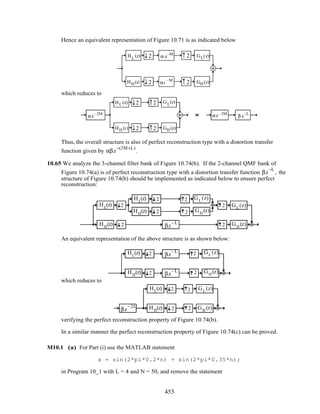
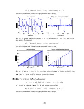
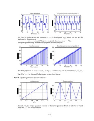
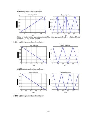
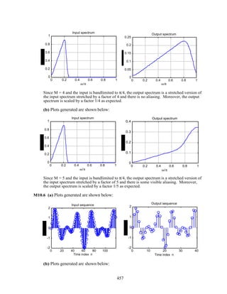
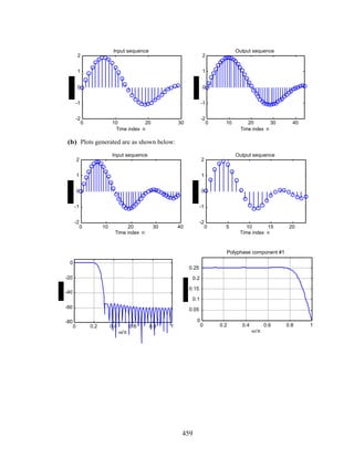
464. 0 0.2 0.4 0.6 0.8 1
0
0.05
0.1
0.15
0.2
0.25
ω /π
Polyphase component #2
0 0.2 0.4 0.6 0.8 1
0
0.05
0.1
0.15
0.2
0.25
ω/π
Polyphase component #3
0 0.2 0.4 0.6 0.8 1
0
0.05
0.1
0.15
0.2
0.25
ω /π
Polyphase component #4
M10.10 As shown in Problem 10.39, a digital lowpass Butterworth half-band filter can be designed
by applying a bilinear transformation to an analog lowpass Butterworth transfer function with a
3-dB cutoff frequency at 1 rad/sec. The 3-dB cutoff frequency of the digital lowpass
Butterworth half-band filter is therefore at ωc = 2tan−1
(1)/ π = 0.5. Thus to design a 5th-order
digital lowpass Butterworth half-band filter we use the MATLAB statement
[num,den]= butter(5,0.5); which yields H(z) =
0.052786(1+ z−1
)5
1+ 0.63344z−2 + 0.055728z−4 . As
can be seen from the pole plot obtained using zplane, all poles are on the imaginary axis.
-1 -0.5 0 0.5 1
-1
-0.5
0
0.5
1
Real part
460

465. Using the pole interlacing property we can express H(z) as H(z) =
1
2
A0(z2
)+ z−1
A1(z2
)( ),
where A0(z) =
0.52786+ z−1
1+ 0.52786z−1 and A1(z) =
0.10557 + z−1
1+ 0.10557z−1 . Hence, H(z) can be realized
using only 2 multipliers.
M10.11 To design a 7th-order digital lowpass Butterworth half-band filter we use the MATLAB
statement [num,den]= butter(5,0.5); which yields
H(z) =
0.016565(1+ z−1
)7
1+ 0.91997z−2 + 0.1927z−4 + 0.0076835z−4 .
As can be seen from the pole plot obtained using zplane, all poles are on the imaginary axis.
-1 -0.5 0 0.5 1
-1
-0.5
0
0.5
1
Real part
Using the pole interlacing property we can express H(z) as H(z) =
1
2
A0(z2
)+ z−1
A1(z2
)( ),
where A0(z) =
0.033131+ 0.68806z−1
+ z−2
1+ 0.68806z−1 + 0.033131z−2 and A1(z) =
0.23191+ z−1
1+ 0.23191z−1 . Hence, H(z) can be
realized using only 3 multipliers.
M10.12 The specifications given are Ws = 0.55π and δs = 0.01. Hence, Wp = 0.45π and
δp = 1 − 1 − δs
2
= 0.0000005. Therefore, Rp = −20log10(1− δp ) = 4.3429 × 10−6
dB and
Rs = −20 log10 (δs ) = 60 dB. Using the commands
[N,Wn] = ellipord(wp, ws, Rp, Rs) and
[b,a] = ellip(7, Rp, Rs, Wn) we then determine the transfer function of an N-th
order elliptic filter and plot its pole locations using zplane(b). The poles of the transfer
function generated are not on the imaginary axis. We next adjust the value of δs and found
that for δs = 0.01 the poles of the transfer function H0(z)generated are on the imaginary axis.
Using the pole interlacing property we can express H0(z) as H0(z) =
1
2
A0(z2
) + z−1
A1(z2
)( ),
461

466. whereA0(z) =
0.1657 +1.0544z−1
+ z−2
1+ 1.0544 z−1
+ 0.1657 z−2 and A1(z) =
0.5559 + z−1
1+ 0.5559z−1 . Thus, the half-band
lowpass elliptic filter is given by H0(z) =
1
2
0.1657 + 1.0544z−2
+ z−4
1 +1.0544z−2
+ 0.1657 z−4 + z−1 0.5559 + z−1
1+ 0.5559z−1





 ,
Its power-complementary highpass transfer function is then
H1(z) =
1
2
0.1657 + 1.0544 z−2
+ z−4
1+ 1.0544z−2
+ 0.1657z−4 − z−1 0.5559 +z−1
1+ 0.5559z−1





 , The gain responses of H0(z) and
H1(z) are shown below:
-1 -0.5 0 0.5 1
-1
-0.5
0
0.5
1
Real part
0 0.2 0.4 0.6 0.8 1
-60
-50
-40
-30
-20
-10
0
ω/π
M10.13 Replace win = hamming(N) with win = hanning(N) in Program 10_8. The
gain response of the 6th-band filter of length 43 is shown below:
0 0.2 0.4 0.6 0.8 1
-80
-60
-40
-20
0
ω/π
M10.14 The specifications of the corresponding zero-phase half-band filter are as follows:
stopband edge ωs = 0.65π and a minimum stopband attenuation of αs = 56 dB. The desired
stopband ripple is therefore δs = 0.0016. The passband edge of the filter is at
ωp = π − 0.65π = 0.35π.Using the function remezord we then estimate the order of F(z) and
using the function remez we next design Q(z). To this end the code fragments used are
[N,fpts,mag,wt] = remezord([0.35 0.65],[1 0],[0.0016 0.0016]);
462

467. The order of F(z) is found to be 19. The next number which is of the form 4K+2 is N = 22,
therefore we use N = 22 to determine H0(z) which will be of order 11 . The filter Q(z) is
designed using the statement
[q, err] = remez(22,fpts, mag, wt);
To determine the coefficients of the filter F(z) we add err to the central coefficient q[12]. Next,
using the function roots, we determine the roots of F(z) which should theoretically exhibit a
mirror image symmetry with respect to the unit circle with double roots on the unit circle.
Choosing the roots inside the unit circle along with the roots on the unit circle we get the
minimum-phase spectral factor H0(z)). The coefficients of H0(z) are as follows:
The coefficients of are
Columns 1 through 6
0.19902 0.47583 0.42992 0.040154 -0.18235 -0.036342
Columns 7 through 12
0.095385 0.015368 -0.050690 -0.0011198 0.025506 -0.010676
The highpass analysis filter H1(z) can be obtained using the following MATLAB
statements
k = 0:11;
h1 = ((-1).^k).*h0;
The synthesis filters can be obtained from the analysis filters using the commands
g0 = fliplr(h0);
g1 = fliplr(h1);
The gain responses of the two analysis filters are shown below:
0 0.2 0.4 0.6 0.8 1
-80
-60
-40
-20
0
20
ω/π
H0
(z) H1
(z)
M10.15 The following MATLAB programs can be used to design the analysis filters corresponding
to a two-channel QMF paraunitary lattice filter bank. (The program uses the function fminu
from the MATLAB Optimization Toolbox, which in turn uses the functions cubici2,
cubici3, optint, searchq, and updhess.)
% Program for the design of a two-channel QMF
% lattice filter bank.
Len = input('The length of the filter = ');
if (mod(Len,2) ~= 0)
sprintf('Length has to be an even number')
463

468. Len = Len+1;
end
ord = Len/2-1;
ws = 0.55*pi;
kinit = [1;zeros([ord,1])];
% set the parameters for the optimization routine
options = foptions;
options(1) = 1;
options(14) = 2500; % maximum number of iterations for the
optimization routine
kfin = fminu('filtopt',kinit,options,[],Len,ws);
e00old = 1;
e01old = kfin(1);
e10old = -kfin(1);
e11old = 1;
for k = 2:length(kfin)
e00new = [e00old 0]-kfin(k)*[0 e01old];
e01new = kfin(k)*[e00old 0]+[0 e01old];
e10new = [e10old 0]-kfin(k)*[0 e11old];
e11new = kfin(k)*[e10old 0]+[0 e11old];
e00old = e00new;
e01old = e01new;
e10old = e10new;
e11old = e11new;
end
E1 = [e00old;e01old];
h0 = E1(:);
scale_factor = abs(sum(h0));
h0 = h0/scale_factor;
E2 = [e10old;e11old];
h1 = E2(:);
h1 = h1/scale_factor;
[H0,W] = freqz(h0,1,1024);
[H1,W] = freqz(h1,1,1024);
plot(W/pi,20*log10(abs(H0)), W/pi, 20*log10(abs(H1)));
grid on
title('Gain response of the analysis filters');
xlabel('omega/pi'); ylabel('Gain, dB');
function val = filtopt(kval,Len,ws)
e00old = 1;
e01old = kval(1);
e10old = -kval(1);
e11old = 1;
for k = 2:length(kval)
e00new = [e00old 0]-kval(k)*[0 e01old];
e01new = kval(k)*[e00old 0]+[0 e01old];
e10new = [e10old 0]-kval(k)*[0 e11old];
e11new = kval(k)*[e10old 0]+[0 e11old];
e00old = e00new;
e01old = e01new;
e10old = e10new;
e11old = e11new;
end
E1 = [e00old;e01old];
h0 = E1(:);
[H0,W] = freqz(h0,1,1024);
val = 0;
464

469. for k = 1:length(W)
if (W(k) > ws)
val = val+abs(H0(k))^2;
end
end
Due to the non-linear nature of the function to be optimized, different values of kinit
should be used to optimize the analysis filter's gain response. The gain responses of the two
analysis filters is as shown below. From the gain response, the minimum stopband attenuation
of the analysis filters is observed to be about 24 dB.
0 0.2 0.4 0.6 0.8 1
-50
-40
-30
-20
-10
0
10
Gain response of the analysis filters
ω/π
M10.16 The MATLAB program used to generate the prototype lowpass filter and the analysis filters
of the 4-channel uniform DFT filter bank is given below:
L = 21; f = [0 0.2 0.3 1]; m = [1 1 0 0]; w = [10 1];
N = 4; WN = exp(-2*pi*j/N);
plottag = ['- ';'--';'-.';': '];
h = zeros(N,L);
n = 0:L-1;
h(1,:) = remez(L-1, f, m, w);
for i = 1:N-1
h(i+1,:) = h(1,:).*(WN.^(-i*n));
end;
clf;
for i = 1:N
[H,w] = freqz(h(i,:), 1, 256, 'whole');
plot(w/pi, abs(H), plottag(i,:));
hold on;
end;
grid on;
hold off;
xlabel('Normalized frequency');ylabel('Magnitude');
title('Magnitude responses of uniform DFT analysis filter
bank');
The plots generated by the above program is given below:
465

470. M10.17 The first 8 impulse response coefficients of Johnston's 16A lowpass filter HL(z) are given by
0.001050167, –0.005054526, –0.002589756, 0.0276414, –0.009666376, –0.09039223,
0.09779817, 0.4810284
The remaining 8 coefficients are given by flipping the coefficients left to right, From Eq.
(10.157), the highpass filter in the tree-structured 3-channel filter bank is given by H2(z) =
z–15HL(z–1). The two remaining filters are given by H0(z) = HL(z)HL(z2) and H1(z) =
HL(z)HH(z2). The MATLAB program used to generate the gain plots of the 3 analysis filters is
given by:
G1 = [0.10501670e-2 -0.50545260e-2 -0.25897560e-2
0.27641400e-1 -0.96663760e-2 -0.90392230e-1 0.97798170e-1
0.48102840];
G = [G1 fliplr(G1)];
n = 0:15;
H0 = (-1).^n.*G;
Hsqar = zeros(1,31); Gsqar = zeros(1,31);
Hsqar(1:2:31) = H0; Gsqar(1:2:31) = G;
H1 = conv(Hsqar,G); H2 = conv(Gsqar,G);
[h0,w0] = freqz(H0,[1]); [h1,w1] = freqz(H1,[1]); [h2,w2] =
freqz(H2,[1]);
plot(w0/pi,20*log10(abs(h0)),'b-',w1/pi,20*log10(abs(h1)),'r-
',w2/pi,20*log10(abs(h2)),'g-.');
axis([0 1 -120 20]);
grid on;
xlabel('Normalized Frequency');ylabel('Gain in dB');
The plots generated are given below:
466

471. 0 0.2 0.4 0.6 0.8 1
-80
-60
-40
-20
0
20
ω/π
H
0
(z)H
1
(z)H
2
(z)
467

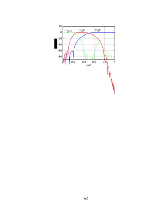
472. Chapter 11 (2e)
11.1 If R = 1250, then the frequency resolution =
7500
1250
= 6 Hz.
If frequency resolution = 4.5 Hz, then R =
7500
4.5
=1667 points.
11.2 (a) resolution =
8000
256
= 31.25 Hz.
(b) We need to take a
8000
16
= 500-point DFT.
(c) resolution =
8000
N
. Hence desired length N of the DFT is given by N =
8000
128
= 62.5.
ince N must be an integer we choose N = 63 as the DFT size.
11.3 (a) F200 =
kFT
R
=
200 ×104
1000
= 2000 Hz, F350 =
kFT
R
=
350×104
1000
= 3500 Hz,
F824 =
kFT
R
=
824×104
1000
= 8240 .
(b) F195 =
kFT
R
=
195×14 ×103
1010
= 2702.97 Hz, F339 =
kFT
R
=
339×14 ×103
1010
= 4699 Hz,
F917 =
kFT
R
=
917×14 ×103
1010
= 12710.89 .
(c) F97 =
kFT
R
=
97×104
517
= 1876.2 , F187 =
kFT
R
=
187× 104
517
= 3617.02 ,
F301 =
kFT
R
=
301×104
517
= 5822.05.
11.4 Let the samples sequence be represented as g[n]= cos(ωo n+ φ). Then, its DTFT is given by
G(ejω
) = π ejφ
δ(ω − ωo + 2πl )+ e− jφ
δ(ω + ωo + 2πl )( )
l =−∞
∞
∑ .
The windowed sequence is given by γ[n] = g[n]⋅w[n] where w[n] =
1, 0 ≤ n ≤ N −1,
0, otherwise.{ The
DTFT of the windowed sequence is then given by
Γ(ejω
) =
1
2
ejφ
ΨR(ej(ω−ωo
)
) +
1
2
e−jφ
ΨR(ej(ω+ωo
)
) where ΨR(ejω
) is the DTFT of w[n] and is
given by ΨR(ejω
) = e−jω(N −1) /2 sin(ωN / 2)
sin(ω / 2)
.
The DFT Γ[k] is a sampled version of Γ(ejω
) sampled at ωk =
2πk
N
. To prevent leakage
phenomenon we require that ωo =
2πl
N
for some integer l . Now ωo =
Ω
FT
where Ω is the

473. angular frequency of the analog signal. If Ω =
2πl FT
N
, then the CTFT Ga(jΩ) of the analog
signal can be determined from Γ[ko].
11.5 ga(t) = cos(200πt). If we require Γ[k]= 0 for all values of k except k = 64 and k = 448, we
require Ωo = 200π to be of the form Ωo =
2πl FT
N
for l = 64. Therefore
200π =
2π × 64 × FT
512
or FT = 800 Hz.
11.6 (a) Fm = 6 kHz. Let FT = 12. The resolution = FT / R. Hence, R =
12000
2.6
= 4616 .
(b) R =
12000
3
= 4000. The closest power-of-2 to 4000 is R = 4096. Hence, a 4096-point FFT
should be used.
11.7 x[n] = A cos(2πf1n / 64)+ B cos(2πf2 n/ 64). Since X[k] = 0 for all values of k except k = 15,
27, 37 and 49, it follows then that either
2π f1
64
=
2π × 15
64
or
2π f1
64
=
2π × 27
64
. Therefore,
f1 =15 or 27.
Case (i): f1 =15 , A = 64, and f2 = 27, B = 32. Therefore,
x[n] = 64 cos(30πn /64)+ 32cos(54πn / 64).
Case (ii): f1 = 27, A = 32, and f2 = 15, B = 64. Therefore,
x[n] = 32cos(54πn / 64)+ 64 cos(30πn / 64).
Thus, there are two possible solutions as indicated above.
11.8 (a) A direct DFT evaluation (no FFT) requires N2
= 250,000 complex multiplications and
N(N − 1) = 249,500 complex additions.
(b) Digital resolution = R =
1
500
= 0.002.
(c) Analog frequency resolution = =
100
500
= 0.2 Hz.
(d) The stopband edge of the filter should be at
FT
2
= 50 Hz.
(e) Digital frequency corresponding to the DFT sample X[31] =
31
500
= 0.062 and that
corresponding to the DFT sample X[390] =
390
500
= 0.78.
Analog frequency corresponding to the DFT sample X[31] = 2π ×
31
500
×100 =12.4π rad/s and
that corresponding to the DFT sample X[390] = 2π ×
390
500
×100 =156π rad/s.

474. (f) length of FFT = 512, and therefore 12 zer-valued samples should be appended.
(g) The FFT sample index that is closest to the old DFT sample X[31] is k = 31 ×
512
500
= 32 and
the FFT sample index that is closest to the old DFT sample X[390] is k = 390 ×
512
500
≅ 399.36
and hence k = 399 is the closest.
11.9 In oder to distinguish two closely spaced sinusoids we require that the separation between the
two frequencies be atleast half of the main-lobe width of the window being used. From Table
7.3, the main-lobe widths of the 4 windows are given by:
(a) Rectangular window: ∆ω =
4π
N
=
4π
60
. Therefore, f2 > f1 +
2
60
= 0.283.
(b) Hamming window: ∆ω =
8π
N
=
8π
60
. Therefore, f2 > f1 +
4
60
= 0.316.
(c) Hann window: ∆ω =
8π
N
=
8π
60
. Therefore, f2 > f1 +
4
60
= 0.316.
(d) Blackman window: ∆ω =
12π
N
=
12π
60
. Therefore, f2 > f1 +
6
60
= 0.35.
11.10 (a) f2 > f1 +
2
110
= 0.268. (b) f2 > f1 +
4
110
= 0.286. (c) f2 > f1 +
4
110
= 0.286.
(d) f2 > f1 +
6
110
= 0.304.
11.11 (a) FT ≥ 2Fm. Hence, the minimum sampling frequency is FT,min = 2Fm.
(b) R =
FT
N
≤ ∆F. Therefore FT ≤ N(∆F). Hence the maximum sampling frequency is
FT,max = N(∆F).
(c) If Fm = 4 kHz, then FT,min = 8 kHz.
If ∆F = 10 Hz and N = 2l
, then FT,max = 2
l
(10).
11.12 (a) XSTFT(e
jω
,n) = x[n – m]w[m]e
−jωm
m=–∞
∞
∑ .
GSTFT(e
jω
,n) = g[n– m]w[m]e
−jωm
m=–∞
∞
∑ = α x[n– m]+ βy[n – m]( )w[m]e
−jωm
m=–∞
∞
∑
= α x[n – m]w[m]e
−jωm
m=–∞
∞
∑ + β y[n – m]w[m]e
−jωm
m=–∞
∞
∑ = α XSTFT(e
jω
, n) + βYSTFT(e
jω
, n).

475. (b) y[n] = x[n – no]. Hence, YSTFT(e
jω
,n) = y[n – m]w[m]e
−jωm
m=–∞
∞
∑
= x[n – no − m]w[m]e
−jωm
m=–∞
∞
∑ = XSTFT(e
jω
,n – no ).
(c) y[n] = e
jωo x[n]. Hence, YSTFT(e
jω
,n) = y[n – m]w[m]e
−jωm
m=–∞
∞
∑
= x[n − m]w[m]e
−j(ω−ωo
)m
m=–∞
∞
∑ = XSTFT(e
j(ω−ωo
)
,n).
11.13 XSTFT(e
jω
,n) = x[n – m]w[m]e
−jωm
m=–∞
∞
∑ . Replacing m in this expression with n – m we
arrive at XSTFT(e
jω
,n) = x[m]w[n – m]e
−jωn
e
−jωm
m=–∞
∞
∑ = e
−jωn
x[m]w[n – m] e
−jωm
m=–∞
∞
∑
e
−jωn
XSTFT(e
−jω
,n). Hence, XSTFT(e
jω
,n) = e
−jωn
XSTFT(e
−jω
,n). Thus, in computing
XSTFT(e
jω
,n) the input x[n] is shifted through the window w[n], whereas, in computing
XSTFT(e
jω
,n) the window w[n] is shifted through the input x[n].
11.14 XSTFT(e
jω
,n) = x[m]w[n – m]e
−jωm
m=–∞
∞
∑ . Hence, by inverse DTFT we obtain
x[m]w[n− m] =
1
2π
XSTFT(e
jω
,n)
0
2π
∫ e
jωm
dω. Therefore,
x[m]w[n− m]
n =–∞
∞
∑ =
1
2π
XSTFT(e
jω
, n)
n=–∞
∞
∑
0
2π
∫ e
jωm
dω, which is equivalent to
x[m] w[n − m]
n =–∞
∞
∑ = x[m]W[0]=
1
2π
XSTFT(e
jω
,n)
n =–∞
∞
∑
0
2π
∫ e
jωm
dω, where
W[0]= w[n – m]
n=–∞
∞
∑ = w[n]
n =–∞
∞
∑ or x[m]=
1
2π W[0]
XSTFT(e
jω
,n)
n=–∞
∞
∑
0
2π
∫ e
jωm
dω.
11.15 From the alternate definition of the STFT given i Problem 11.13 we have
XSTFT(ejω
,l ) = x[m]w[l − m]e−jωm
m=−∞
∞
∑ . Therefore,

476. XSTFT(ejω
,l)ejωn
l =−∞
∞
∑ = x[m]w[l − m]e−jω(m−n)
m=−∞
∞
∑
l =−∞
∞
∑ . Hence,
XSTFT(ejω
,l )ejωn
l =−∞
∞
∑ dω
0
2π
∫ = x[m]w[l − m] e−jω(m−n)
0
2π
∫m=−∞
∞
∑
l =−∞
∞
∑ dω .
Now, ejωk
dω
0
2π
∫ =
2π, if k = 0,
0, if k ≠ 0.{ Thus,,
x[m]w[l − m]⋅2π δ[m − n] =
m=−∞
∞
∑
l =−∞
∞
∑ XSTFT(ejω
,l )ejωn
l =−∞
∞
∑ dω
0
2π
∫ , or
2π w[l − n]
l =−∞
∞
∑ ⋅x[n]= XSTFT(ejω
,l )ejωn
l =−∞
∞
∑ dω
0
2π
∫ .
Let W[0]= w[n].
n=−∞
∞
∑ Then x[n] =
1
2π W[0]
XSTFT(ejω
,l )ejωn
l =−∞
∞
∑ dω
0
2π
∫ .
11.16 XSTFT(e
jω
,n) = x[n – m]w[m]e
−jωm
m=–∞
∞
∑ . Hence,
XSTFT[k,n]= x[n – m]w[m]e
−j2πkm / N
m=–∞
∞
∑ = x[n] * w[n]e
−j2πkn / N
. Or in other words,
XSTFT[k,n] can be obtained by filtering x[n] by an LTI dystem with an impulse response
hk[n] = w[n]e
−j2πkn / N
as indicated in Figure P11.1.
11.17 XSTFT(e
jω
,n) = x[n – m]w[m]e
−jωm
m=–∞
∞
∑ . Hence,
XSTFT(e
jω
, n)
2
= x[n – m]x[n –s]w[m]w[s]e
−jωm
e
−jωs
m=–∞
∞
∑
s=–∞
∞
∑ . Thus,
r[k,n] =
1
2π
XSTFT(e
jω
,n)
2
e
jωk
dω
0
2π
∫ = x[n– m]x[n– s]w[m]w[s]δ[s + k − m]
m=–∞
∞
∑
s=–∞
∞
∑
= x[n – m]x[n – m + k]w[m]w[m − k]
m=–∞
∞
∑ .
11.18 (a) Length of the window N = FT τ

477. (b) The number of complex multiplications is C =
N
2
log2 N =
FTτ
2
log2(FTτ). An FFT is
performed after every K amples, i.e after every K / FT seconds. Thus, the number of complex
multiplications per second is
C
K / FT
=
FT
2τ
2K
log2(FT τ).
11.19 ϕST[k,n]= x[m]w[n − m]x[m+ k] w[n − k − m].
m=–∞
∞
∑
(a) ϕST[− k,n] = x[m]w[n − m]x[m − k]w[n + k − m].
m=–∞
∞
∑
Substitute in the above expression m – k = s, i.e. m = k +s. This yields
ϕST[−k,n] = x[s + k]w[n − k − s]x[s]w[n − s]= ϕST[k,n].
s=–∞
∞
∑
(b) Let m + k = s. Then, ϕST[k,n]= x[s − k]x[s]w[n −s + k] w[n− s]
s=–∞
∞
∑ . It follows from
this expression that ϕST[k,n] can be computed by a convolution of hk[n] = w[n]w[n+k] with
x[n]x[n – s] as indicated in Figure P11.2.
11.20
S(z)
z
–1
α
1 – α
2
– α
X(z) Y(z)
Analysis yields S(z) = αz
–1
S(z)+ X(z), and Y(z) = –α X(z) + (1− α
2
)z
−1
S(z). Solving the
first equation we get S(z) =
X(z)
1− αz
−1 , which when substituted in the second equation yields
after some algebra
Y(z)
X(z)
=
−α + z
−1
1− αz
−1 . The transfer function is thus seen to be a Type 1
allpass of the form of Eq. (6.58) and can thus be realized using any one of the single-
multiplier structures of Figure 6.36.
11.21 Analysis of the structure of Figure P11.4 yields
Y(z)
X(z)
=
−α + z
−1
A(z)
1− αz
−1
A(z)
, where A(z) denotes the
transfer function of the "allpass reverberator". Note that this expression is similar in form to
that of Eq. (6.58) with "d" replaced by "− α " and "z–1" replaced by "z–1A(z)". Hence an
efficient realization of the structure of Figure P11.4 also is obtained readily from any one of
the structures of Figure 6.36. One such realization is indicated below:

478. X(z)
Y(z)
z–1
–1
− α
A(z)
11.22 G2(z) =
K1
2
1− A2(z){ }+
K2
2
1+ A2 (z){ } = K2
1
2
K1
K2
1− A2 (z){ }+
1
2
1+ A2 (z){ }








.
Hence in this case, the ratio K1/K2 determines the amount of boost or cut at low frequencies,
K2 determines the amount of dc gain or attenuation at all frequencies, α determines the
3-dB bandwidth ∆ω3−dB = cos−1 2α
1+ α2





 ,and the center frequency ωo is related to β
through β = cosωo .
alpha = 0.8;
beta = 0.4;
K1 = [0.9];
K2 = [0.5 2];
nbp = ((1-alpha)/2)*[1 0 -1];
dbp = [1 -beta*(1+alpha) alpha];
nbs = ((1+alpha)/2)*[1 -2*beta 1];
dbs = dbp;
[Hlp,w] = freqz(nbp,dbp,512);
[Hhp,w] = freqz(nbs,dbs,512);
hold on
for k = 1:length(K1)
for m = 1:length(K2)
H = K1(k)*Hlp+K2(m)*Hhp;
semilogx(w/pi,20*log10(abs(H)));
xlabel('Gain, dB');
ylabel('omega/pi');
clear H;
hold on;
end
end
grid on
axis([.01 1 -8 8]);
11.23 The transpose of the decimator structure of Figure 11.63 yields

479. 3
3
3
3
3
3
z–1
z–1
z–1
z–1
z –1
z–1
2
2
E00(z)
E01(z)
E02(z)
E12(z)
E11(z)
E10(z)
x[n]
y[n]
11.24
H(z)3 4
3 4
3
3
z−1
z−1
R0(z)
R1(z)
R2(z)
3 4
3
3
R0(z)
R1(z)
R2(z)
z−4
z−4
z
3
z
6
(a) (b)
z
−1
z
−1
3 4
3
3
R0(z)
R1(z)
R2(z)
4
4
z
z
z−1
z−1
34
3
3
R0 (z)
R1(z)
R2 (z)
4
4
z−1
z−1
(c) (d)

480. z−1
z−1
34
3
3
4
4z−1
z−1
z−1
z−1
z−1
z−1
z−1
z
−1
z−1
z−1
z−1
4
4
4
4
4
4
4
4
4
E20 (z)
E21(z)
E22 (z)
E23 (z)
E10 (z)
E11(z)
E12 (z)
E13(z)
E00 (z)
E01 (z)
E02 (z)
E03 (z)
(e)
M11.1 Figures below illustrate the application of Program 11_1 in detecting the touch-tone digits A
and 3:
Touch-Tone Symbol = A Touch-Tone Symbol = 3
M11.2 For R = 16, the two strong peaks occur at k = 3 and 5. The associated frequencies are
ω1 =
2π×3
16
, or f1 =
3
16
= 0.1875, and f2 =
5
16
= 0.3125. For R = 32, the two strong peaks occur at
k =5 and 10. The associated frequencies are f1 =
5
32
= 0.15625, and f2 =
10
32
= 0.3125.

481. For R = 64, the two strong peaks occur at k = 11 and 22. The associated frequencies are
f1 =11/ 64 = 0.1718, and f2 = 20/ 64 = 0.3125. For R = 128, the two strong peaks occur at k =
21 and 39. The associated frequencies are f1 = 21/128 = 0.1641, and f2 = 39 /128 = 0.3047.
Moreover, the last two plots show a number of minor peaks and it is not clear by examining
these plots whether or not there are other sinusoids of lesser strengths present in the sequence
being analyzed.
An increase in the size of the DFT increases the resolution of the spectral analysis by reducing
the separation between adjacent DFT samples. Also the estimated values of the frequencies of
the sinusoid get closer to the actual values of 0.167 and 0.3076 as the size of the DFT increases.
M11.3 As the separation between the two frequencies decreases, the distance between the two
maximas in the DFT of the sequence decreases, and when f2 = 0.21, the second sinusoid
cannot be determined from the DFT plot. This is due to the use of a length-16 rectangular
window to truncate the original infinite-length sequence. For a length-16 rectangular
window, two adjacent sinusoids can be distinguished if their angular frequencies are apart by
half the mainlobe width of
4π
N
radians or equivalently, if their frequencies are apart by
2
N
= 0.0625. Note that the DFT length R = 128 is all plots.

482. M11.4 f2 = 0.21, f1 = 0.18. Hence, ∆f = 0.03. For a Hamming window the mainlobe width
∆ML =
8π
N
. The DFT length R = 128 in all plots.
(i) N = 16. Here it is not possible to distinguish the two sinusoids. This also can be seen
from the value of ∆ML =
8
16
= 0.5, and hence, half of the mainlobe width is greater than ∆f .
(ii) Increasing N to 32, makes the separation between the two peaks visible. However, it is
difficult to identify the peaks accurately.

483. (iii) Increasing N to 64, makes the separation between the two peaks more visible. However,
it is still difficult to identify the peaks accurately.
(iv) For N = 128, the separation between the two peaks clearly visible.
Note also the suppression of the minor peaks due to the use of a tapered window.
M11.5 Results are similar to that in Problem M11.4.
M11.6 f2 = 0.21, f1 = 0.18. Hence, ∆f = 0.03. The DFT length R = 128 in all plots.

484. (i) For N = 16, it is difficult to identify the two sinusoids.
(ii) For N = 32, there are two peaks clearly visible at k = 36 and 43, respectively.
(iii) For N = 64, it is difficult to identify the two sinusoids.
(iv) For N = 128, there are two peaks clearly visible at k = 37 and 41, respectively.
M11.7

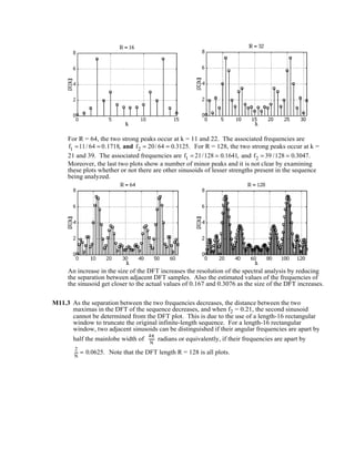
485. The SNR computed by the program is –7.4147 dB. There is a peak at the frequency index 29
whose normalized frequency equivalent is equal to 29/256 = 0.1133. Hence the DFT approach
has correctly identified the frequency of the sinusoid corrupted by the noise.
M11.8
The SNR computed by the program is –7.7938 dB. There is a peak at the frequency index 42
whose normalized frequency equivalent is equal to 42/256 = 0.1641. Hence the DFT approach
has correctly identified the frequency of the sinusoid corrupted by the noise.
M11.9 The following program can be used to plot the power spectrum estimates of the noise
corrupted signal windowed by a rectangular window.
% Power Spectrum Estimation %
nfft = input('Type in the fft size = ');
n = 0:1000;
g = sin(0.1*pi*n) + sin(0.2*pi*n) + randn(size(n));
window = boxcar(nfft);
[Pxx, f] = psd(g,nfft,2,window);
plot(f/2,10*log10(Pxx));grid
xlabel('omega/pi');ylabel('Power Spectrum, dB');
titletext=sprintf('Power Spectrum With Window Size =
%d',nfft);
title(titletext);

486. The power spectrum estimate with window size = 64 and 256 are shown below
0 0.1 0.2 0.3 0.4 0.5
-5
0
5
10
15
ω/π
Power Spectrum With Window Size = 64
0 0.1 0.2 0.3 0.4 0.5
-10
-5
0
5
10
15
20
ω/π
Power Spectrum With Window Size = 256
M11.10 Program_11_4 can be used to evaluate the Bartlett and Welch estimate by changing
g = 2*sin(0.12*pi*n) + sin(0.28*pi*n) + randn(size(n));
to g = sin(0.1*pi*n) + sin(0.2*pi*n) + randn(size(n));
and the line window = hamming(256) with window = boxcar(1024) for the
Bartlett estimate, and with window = hanning(1024) for the Welch estimate. Also set
nfft=1024.
The plot of the Bartlett estimate of the power spectrum estimate for the noise corrupted signal
is shown below
0 0.1 0.2 0.3 0.4 0.5
-30
-20
-10
0
10
20
30
ω/π
Bartlett Estimate (Overalp = 0 samples)
The Welch estimates of the power spectrum with an overlapping Hann window for overlaps of
64 and 128 samples are shown below

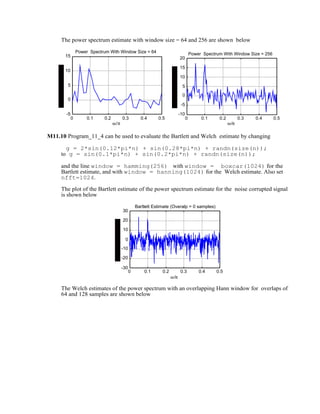
487. 0 0.1 0.2 0.3 0.4 0.5
-30
-20
-10
0
10
20
30
ω/π
Welch Estimate (Overalp = 64 samples)
0 0.1 0.2 0.3 0.4 0.5
-30
-20
-10
0
10
20
30
ω/π
Welch Estimate (Overalp = 128 samples)
M11.11 Use the statement b = remez(11,[0 0.3 0.5 1],[1 1 0 0],[1 1]); to
design the FIR filter. Then use the statement [d,p0] = lpc(b,order); and run it for
order = 4,5 and 6 to determine an equivalent all-pole model. The magnitude response of the
orignial FIR filter (solid line) and the all-pole equivalent (dotted line) are shown below for
different values of order.
0 0.2 0.4 0.6 0.8 1
0
0.5
1
1.5
ω/π
Order of all-pole equivalent = 4
Original
Estimate
0 0.2 0.4 0.6 0.8 1
0
0.5
1
1.5
ω/π
Order of all-pole equivalent = 5
Original
Estimate
0 0.2 0.4 0.6 0.8 1
0
0.5
1
1.5
ω/π
Order of all-pole equivalent = 6
Original
Estimate