Downloaded 413 times
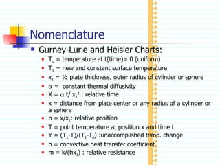
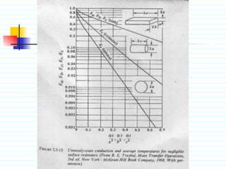
![Nomenclature Chart for Semi-infinite solid Semi-infinite solid – solid where the unidirectional conductive heat transfer is infinite (Ex. Ground) T o = initial uniform solid temperature T 1 = constant ambient temperature to which solid surface is exposed T = temperature of solid at position x 1- Y = (T-T o )/(T 1 -T o ): Ordinate h( t) 0.5 /k : convective parameter x/[2 ( t) 0.5 ]: Abscissa](https://image.slidesharecdn.com/unsteady-state-basics-1229913196450954-2/85/Unsteady-State-Basics-10-320.jpg)
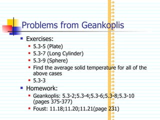
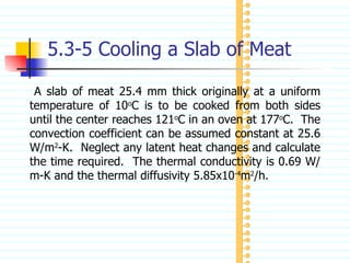
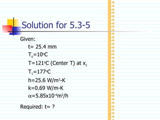
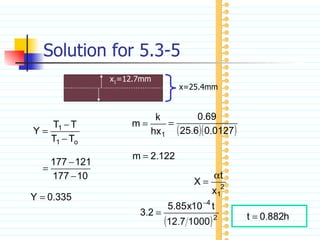
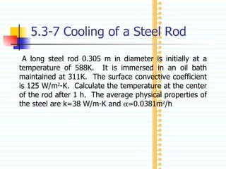
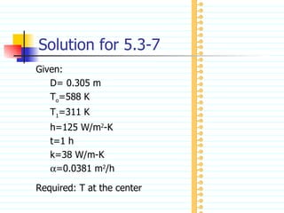
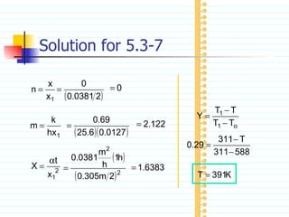
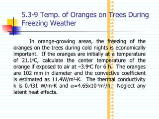
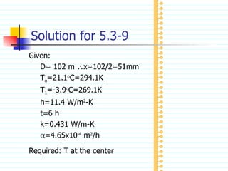
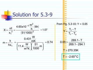
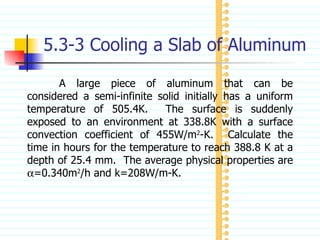
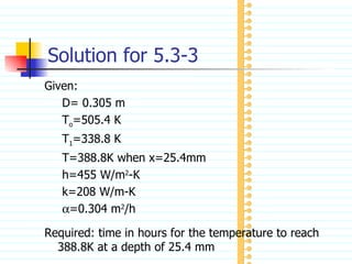
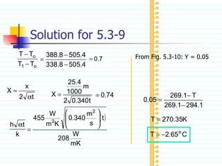
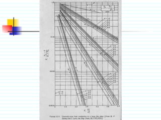
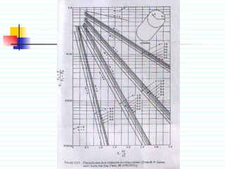
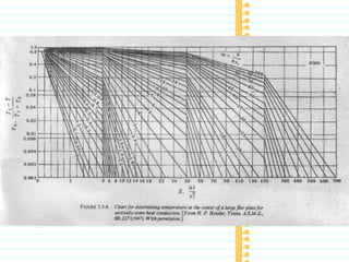
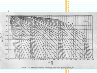
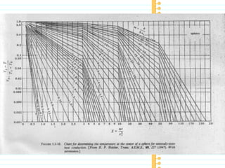
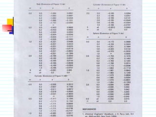

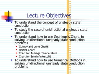
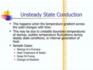
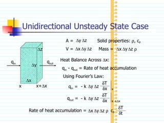
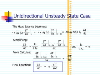
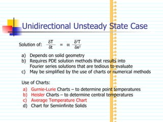
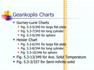
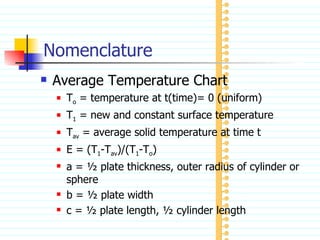
The document discusses unsteady state heat conduction, which occurs when the temperature gradient across a solid changes over time. It provides examples of unsteady state conduction and examines the one-dimensional case. It introduces the governing equation and describes using charts like the Geankoplis charts to solve problems involving startup conditions for plates, cylinders, and spheres. It then provides examples of using the charts to solve problems involving cooling/heating of various objects.