A polynomial function is a function of the form f(x) = anxn + an-1xn-1 + ... + a2x2 + a1x + a0, where each coefficient ak is a real number, an ≠ 0, and n is a non-negative integer. The degree of a polynomial is determined by the highest exponent of x, and the leading coefficient is the coefficient of the term with the highest exponent. Polynomial functions can be classified as increasing or decreasing based on whether higher x-values result in higher or lower y-values. Polynomials have local and absolute extrema, turning points, and their graphs can be sketched based on x-intercepts and evaluating the function at

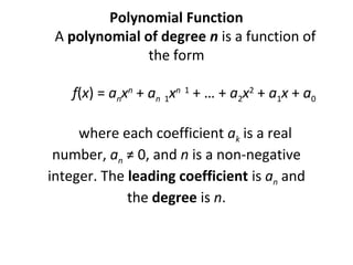
1.
Polynomial Function
A polynomial of degree n is a function of
the form
f(x) = anxn + an 1xn 1 + … + a2x2 + a1x + a0
where each coefficient ak is a real
number, an ≠ 0, and n is a non-negative
integer. The leading coefficient is an and
the degree is n.

2. • Below are the graphs of some degree 3 and
degree 4 polynomials. Notice that both are
smooth (like a parabola), but have more
curves. We shall examine how many curves a
polynomial can have a little later on.
•

4. •
•
•
•
•
•
•
Example 1:
What are the degree and leading coefficients
of the following polynomials?
(i) 10x3 + 4x2 + 3x + 1 and (ii) 2x4 + 3x + 5

5. • Solution:
•
• For (i), we see that the degree is 3 and the
leading coefficient is 10. For (ii), we see that
the degree is 4 and the leading coefficient is 2.
• At this point, it is useful to introduce two
more concepts about functions that will help
us to describe their graphs better.

6. •
•
•
•
•
•
•
•
•
•
Increasing and Decreasing Functions
Suppose that f(x) is a function defined over an interval I on the
number line. If x1 and x2 are in I, then we say that
f(x) increases on I if, whenever x1 < x2, f(x1) < f(x2)
and
f(x) decreases on I if, whenever x1 < x2, f(x1) > f(x2)

8. •
•
•
•
Example 2:
Use the graph of f(x) = 12x x3 (shown
below) to identify the intervals where f(x) is
increasing and decreasing.

10.
Solution:
From the graph, we see that f(x) is
increasing on the interval (-2, 2) and
decreasing on the intervals (-∞, -2) (2, ∞).
•
•
•
•
•

11. •
•
•
•
•
•
•
•
Let us take a closer look at the graph above. The places where the graph
changed from increasing to decreasing and from decreasing to increasing are of
particular importance in calculus. We shall call those pointsturning points, since
the graph changes direction. In calculus, one can show that a polynomial of
degree n has at most n 1 turning points.
While we are considering graphs of polynomials, it is worth mentioning some
additional concepts. In particular, notice that there were two types of turning
points. One that appeared at “the top of the hill” and the other which appeared at
“the bottom of the valley”. More formally, we call those points a local maximum
and a local minimum of the graph.
We may also be interested in determining the largest or smallest value of the
function overall. We call those points the absolute maximum and absolute
minimum, respectively.
To recap, we have the following:

12. •
•
•
•
•
•
•
•
•
Absolute and Local Extrema
Suppose c is in the domain of f(x). Then
(i) f(c) is an absolute (global) maximum if f(c) ≥ f(x) for all x in
the domain of f(x)
(ii) f(c) is an absolute (global) minimum if f(c) ≤ f(x) for all x in
the domain of f(x)
(iii) f(c) is a local (relative) maximum if f(c) ≥ f(x) when x is near c
(iv) f(c) is a local (relative) minimum if f(c) ≤ f(x) when x is near c
Note: By “near c”, we mean that there is an open interval in the
domain of f(x) containingc, where f(c) satisfies the stated inequality.

13. •
•
•
•
•
Example 3:
Below is the graph of f(x) on the interval [-3,
4]. Use the graph to identify the points where f(x)
has a local maximum and local minimum. Also
identify the absolute maximum and absolute
minimum of f(x) on the interval.

15.
Solution:
We observe that there is a local maximum at
the point (1, 37) (with a value of 37). There are
two local minimums, occurring at (-2, -152) and
(3, -27) (with values -152 and -27, respectively).
On the interval [-3, 4], the maximum value is 64
(and occurs at (4, 64)) and the minimum value is
-152 (and occurs at (-2, -152)).
•
•
•
•
•

16. •
•
•
•
•
•
•
•
Finally, we turn our attention to graphing polynomials. If we have a
polynomial in factored form, we can make a rough sketch of the graph by
considering the following three steps.
List all of the x-intercepts of the graph and (lightly) draw vertical lines at
those intercepts.
Choose points to the left and to the right of each intercept and determine
if the function is positive or negative. (Whenever possible, it is preferable
to choose integers, as the math is usually simpler.) Plot the points on the
graph. (You may wish to shade the area in between the x-intercepts that
the chosen point does not pass through. These are known as the excluded
regions.)
Finally, draw a smooth curve between the points you have drawn.
This is best illustrated through an example.

17. •
•
•
•
Example 4:
Sketch a graph of f(x) = (x + 4)(x 1)(x 4).

18. • Solution:
•
• We begin by plotting the x-intercepts of the
graph (which occur at x = -4, 1, and 4) and
draw in light vertical lines at those points.
•

20. • Next, we choose points in between the
dashed lines. For the sake of simplicity, we
shall choose x = -5, x = -2, x = 2, and x = 5.
Notice that f(-5) = -54, f(-2) = 36, f(2) = -12,
and f(5) = 36. Plotting those points on the
graph, we have the following.
•
•

22. • We place shaded rectangles to show the
places where the graph does not pass
through. Also, at this point, we can remove
our vertical lines. Doing so, we have the
following:
•

24. • Finally, we draw a smooth curve that
connects the points, making sure not to cross
into any of the shaded regions. Doing this, we
have:
•

26. • And finally, we remove our shaded regions to
obtain our final graph.

28. • In the example above, the polynomial had no
repeated factors. That is, none of the factors
is squared or cubed or so on. But what
happens if there are repeated factors. Again,
we shall follow the three steps listed above.
But there is a fact from calculus that will aid
us.
•

29. •
The Behavior of a Polynomial Function near
an x-intercept
• Let f(x) be a polynomial and suppose that
(x a)n is a factor of f(x). Then, in the immediate
vicinity of the x-intercept at a, the graph
of y = f(x) closely resembles that of y = A(x a)n.
•

30. • Drawn below are the graphs of y = (x + 1)
(x 1)(x 2), y = (x + 1)2(x 1)(x 2), and y = (x +
1)3(x 1)(x 2).
•

32. • In the first graph, notice that near the xintercept of -1, the function looks like a
straight line. In the second graph, near the xintercept of -1, the function looks like a
parabola, and in the third graph, near the xintercept of -1, the function looks like a cubic.
•