An Advanced learning FEA, CAE - Ansys, Inventor CAM

CAE Assignment
Submitted by
Anglia Ruskin University
SID 1227201

1
Contents
Pre-Requisites:.............................................................................................................................................................................................3
Workbook A part 2:.....................................................................................................................................................................................4
Exercise 2.1a............................................................................................................................................................................................4
Exercise 2.1b............................................................................................................................................................................................6
Exercise 2.1c.......................................................................................................................................................................................... 13
Exercise 2.2............................................................................................................................................................................................14
Exercise 2.3............................................................................................................................................................................................15
Exercise 2.4............................................................................................................................................................................................17
Exercise 2.5............................................................................................................................................................................................18
Workbook Part B:......................................................................................................................................................................................22
Given to us.............................................................................................................................................................................................22
To Obtain............................................................................................................................................................................................... 22
Methodology:............................................................................................................................................................................................23
Inventor Design:........................................................................................................................................................................................ 24
Base Design:.......................................................................................................................................................................................... 24
Iteration 1..................................................................................................................................................................................................25
Result:....................................................................................................................................................................................................26
Iteration 2..................................................................................................................................................................................................27
Result:....................................................................................................................................................................................................29
Iteration 3..................................................................................................................................................................................................30
Result:....................................................................................................................................................................................................32
Final Part....................................................................................................................................................................................................33
Meshing Analysis...................................................................................................................................................................................34
Result:....................................................................................................................................................................................................38
Manufacturing Model - CNC..................................................................................................................................................................... 39
Results (Physical Test)............................................................................................................................................................................... 41
Physical Part.......................................................................................................................................................................................... 41
Zoomed view of the necking.................................................................................................................................................................42
Testing........................................................................................................................................................................................................43
Validation...................................................................................................................................................................................................45
Conclusion................................................................................................................................................................................................. 46
References................................................................................................................................................................................................. 47

2
Introduction:
CAE is an essential part in understanding the world of designing and manufacturing engineering products. Every product that is
designed, developed on 3d sketch is analysed on FEA (Finite Element Analysis). This saves time & money for the companies. On the
other hand this increases the efficiency rate, meeting the demands on time. FEA produces, exact similar results that are obtained in
physical tests. Most of the engineering companies these days use with variation of FEA soft wares like ANSYS, CAELinux,
NASTRAN/PATRAN (often used by NASA) Abaqus (Dassult Systems) & many more as you name it.
FEA not only helps in breaking the results in computerized method for predicting the solutions but also helps in understanding how
the product behaves under real world forces, vibrations, static & dynamic forces and other physical as well as boundary conditions
(Auto Desk, U.S. 2014) (Figure 1)
More or less, this has become an essential part in engineering which has not only made engineering problems an easy approach but
has encouraged more flexibility in resolving to solutions of the problems.
Figure 1 CAE analysis figure

3
Pre-Requisites:
The assignment requires a basic understanding of how to design a product on Inventor Professional 2014 (AutoDesk) (refer work
book A) or any similar designing software like CATIA, Inventor Fusion or linux softwares like libreCAD. Using Ansys workbench for
static analysis of the part. Applying forces, displacement, understanding of meshing and deriving results like equivalent von mises
stress, Safety factor. (Refer Work book A). Standard long hand calculations for the confirmation of the results obtained by the physical
tests & from ANSYS workbench. Calculating the tensile stress from the graph and changing engineering data on workbench.

4
Workbook A part 2:
Exercise 2.1a
Given:
An element which is drawn in the Autodesk inventor,
and extruded shown in figure . To execute the
simulation of the part in FEA analysis in ANSYS .
Solution and explanation:
Meshing refers to a geometrical representation of set of fine elements. This feature allows to split the whole design in a set of the
fine structures that analyze the stress and deformation to combine and produce a perfect set of results like the equivalent stress,
strain or deformation of a part designed. Meshing plays an important role in the Finite Element Analysis (FEA) ANSYS to understand
the part designed. It is an important and critical part of engineering. This feature provides the balance to the requirements and the
right mesh in each simulation (ANSYS, 2014). However the mesh size can be changed and varied according to the requirement.
Figure 2 Inventor drawing
Figure 3 25 mm Mesh size
Figure 4 Element quality %

5
Comments:
The above part is meshed in 25 elements. Meshing results can be seen as in figures 3 & 4.
 After meshing it is found that 77 percent of the elements as volume fall in between 88% to 97% of fine mesh quality. However
there are approximately 1% each which is categorized as in between 50% to 80% mesh quality each.
 Again the are ill conditioned elements in the meshing.
 Similarly the other factor which results as a perfect mesh is the aspect ratio which is the ratio of length to breadth of a mesh
(Longer side/ shorter side).
Figure 5 Aspect ratio
 The aspect ratio should result in more mesh greater than 0.8 ie. 70% of them should be > 0.8
 However here we have 77.69% of the mesh greater than 1.20 but more spread out in more than 4 to 8 .
Hence forth ion consideration with the above factors and results, it can be concluded that the mesh is not good and may not result in
accurate variable factors like stress, strain and deformation.
Figure 6 Element quality at 20 mm

6
To have a perfect quality of mesh it is advisable to have at least 3 layers of meshing of the part. This tends to achieve the best results
which simulating the design.
Exercise 2.1b
Skweness is primary used to determine the quality of the mesh. It usually determines how close the element to the ideal ones is.
Extremely high skewed elements are never acceptable in FEA analysis.
Aspect ratio refers to the ratio of the longer side to the shorter side of the mesh, ie. l/b . It is acceptable to have 70% of the mesh
with Aspect ratio < 4 & Element quality 70% of mesh > 0.8
Given:
A T beam fixed on the T side (face)
Tensile Force on free end = 1000 N
Thickness = 25 mm
Inventor Drawing and FEA on ANSYS:
Figure 7 Inventor design

7
Mesh element size 25 mm:
Figure 25 mm mesh size
Figure 8 Element quality at 25 mm mesh size
Mesh size in
mm
Aspect Ratio Element quality Skweness
25
With the element size 25 mm , 74 .07
% of the elements by volume lies
between 1.25 to 1.50 where as 20%
and 10 % of them lie in between 2.00
to 2.50 and beyond 4.50.
This clearly indicated that the aspect
ratio is widely scattered
The elements have widely scattered
quality ranging from 0.22 to 0.35 and
again from 0.75 to 0.96.
The Skweness is however less
with average of 0.215
Comment:
This is not a proper meshing. It is because, Skweness is high with almost 67 elements have highly skewed structures in 25 mm
mesh. The aspect ratio and the element quality are widely scattered. The more the elements occur in one strict region the
better the mesh is and the more accurate results are obtained.

8
Figure 9 Mesh element size 20 mm
Skweness at 20 mm
Figure 10 Aspect ratio with 20 mm mesh element size
Figure 11 20 mm mesh element size quality
Comment:
Mesh size in
mm
Aspect Ratio Element quality Skewness
20
Wide spread in region 1.60 - 1.75 ;
2.25 to 2.75. High concentration of
the elements are in the region of
1.65 to 1.69. But all the elements are
less than 4
The elements are scattered around
in between 0.70 to 0.90 . However
79.37 % are restricted at 0.88
element quality.
The skewness starts to
decrease, on an average it is
0.182
It is well noted that with decrease in the mesh size, the Skweness decreases, aspect ratio and element quality improves.
However this is not the best mesh. Further gradual decrease in the mesh size can be done for accuracy.

9
Figure 12 Skweness at element size 15 mm
Figure 13 Aspect ratio at 15 mm mesh element size
Figure 14 Element quality at mesh size 15 mm
Comment:
Mesh size in
mm
15
With high concentration of the
elements - 82.30 % of the entire
volume of the elements of the mesh
lies in the region of 1.45 - 1.46
Similarly 82.30% of the entire
volume of the elements of the mesh
lies in the region of 0.93 to 0.945
On contrast the skewness
increases. On an average the
skewness reaches to 2.68
This is slighter better than comparison to the mesh size 25 mm and 20 mm. With more elements with fixed aspect ratio and the
element quality but increased Skweness. The mesh is still not accurate as more elements can be made to concentrate in one
region rather than scattered. However this can still be accepted as it has at least 2 layers of meshing for better accuracy.

10
Figure 15 Skweness at element size 10 mm
Figure 16 Element Quality at 10mm mesh size
Figure 17 Aspect ratio at 10 mm element size
Comment:
Mesh size in
mm
10
78 number of the elements lie in
the aspect ratio of 1.26 - 1.28 which
is almost more than 70% of the
elements < 4 and is less scattered
Whilst 78 number of elements are
concentrated at 0.95 to 0.96 which is
again 70% of the elements > 0.8 and
very few scattered
Average Skweness is high at
7.84 as the number of the
elements increased and
henceforth the elements
around the joint tries to
achieve the ideal geometry
has also increased.
The mesh size 10 mm can be an acceptable meshing as it constraints certain points of having almost to the accuracy of the
aspect ratio and element quality. However the only one factor that restricts that 10 mm cannot be considered for prefect
results is the Skweness which suddenly changes to very high. Hence it is well understood that we can still try to reduce the
mesh size for near about ideal results.

11
Figure 18 Skweness at element size 5
Figure 19 Aspect ratio at Element size 5 mm
Figure 20 Element quality at 5 mm mesh size
Comments:
Mesh size
in mm
5
100 % of the elements have a good
aspect ratio of 1 which is uniform
across all the elements
All the elements have quality of 1
which is highly acceptable since 100%
= 1
Skewness drastically reduces
to 1.305 on average
The element size can be widely acceptable in contrast to 25, 20, 15 & 10 as this mesh size consists of 3 layers of
meshing. As discussed earlier that any meashing having three layers of mesh results to more accurate result and accounting to
the aspect ratio and element quality all the elements lie in a concentrated region of 1.

12
Mesh element size 1.50 mm:
Figure 21 Skweness at element size 1.50mm

13
Figure 22 Aspect ratio at 1.50 mm element size
Figure 23 Element Quality at 1.50 mm mesh size
Comment:
Below is the distribution of the Skweness in respect to the mesh size. :
Exercise 2.1c
Mesh Element Size in mm Stress in MPa
1.5 83.121
5 60.73
10 63.919
15 59.894
20 59.881
25 Crashed
Mesh size
in mm
1.5
19,992 elements lie in the region of
near about 1.05 and however there
are few elements which lie b/w 1.17 -
1.18
All the elements have quality within
0.99 to 1 but however the
concentration of the elements is
distributed with in that region
Skweness remains same of
about 1.305 as average
Mesh size (mm) Skweness
1.5 1.305
5 1.305
10 7.84
15 2.68
20 0.182
25 0.215
This is an example that always decrease in the mesh size does not affect the aspect ratio or element quality. At 1.5 the aspect ratio
and element quality decreases to more scattered elements however the Skweness remain constant. This may however affect stress
determination using probe at the joint areas.

14
Exercise 2.2
Given:
L = 24 mm
B = 24 mm
H = 6 mm
Diameter of the circle = 5 mm
Force = 2000 N
E = 200,000 MPa (material steel)
Hand Calculation:
There will be stress acting on the plate as well as there will be a stress concentration around the hollow circular area. As the diagram
below explains the formula, we we derive the stress acting in the part.
The tensile force acts uniform along on the side . The initial stress calculation: σ = Force/ Area
Area = t x D ie. = (6 x 24)mm2
= 144 mm2
Henceforth the stress is = (2000/ 144) N/mm2
= 13.8 MPa
But since there is a stress acting adjacent to the hole, which needs to be calculated as above mentioned. This given by
σ max = σ nom x k
σ nom = (D/(D-2r)) x σ

15
σ nom = nominal stress in absence of the stress raiser
k = Stress concentration factor
a = the diameter of the hole
b = the width of the plate
Hence c = a/b
Therefore the calculated c = 5/24 = 0.208 = 0.21
From chart figure
k = 2.5
σ nom = (24/(24-2x2.5))x13.8 = 17.43 N/mm2
σ max = 17.43 x k = 17.43 x 2.5 = 43.57 N/mm2
Or the total σ max = 43.57 MPa
Safety Factor :
S.F. =( Yield Stress / Maximum stress )
(250/ 43.57) = 5.7378
Inventor and FEA Analysis:

16
Figure 24 Ansys Stress diagram and Inventor design
Figure 25 Safety Factor
Inference: The following results were obtained when the part was subjected to ANSYS FEA analysis.
 Maximum stress obtained on simulation is 48.289 MPa
 The total deformation is 0.0019 mm
 The safety factor obtained on simulating the part is 5.1771
Interpretation: With the static load on the free end, there is hardly any visible deformation. Being the material of steel, it has
boundary conditions same and homogeneous properties. There are variables in the geometry as there is a hollow circular region in
the center of the plate, where there are stress concentrations when load is applied. The stress is tensile.
Conclusion: The results obtained on the FEA analysis and the hand calculations are approximately same with minimal variation. This
can a reason of the default mesh quality. However the region of the highest stress is concentrated in a very minute part of 48.289
MPa while the region of 43.352 MPa is spread more. Hence we can concluded the results are validated.
Exercise 2.3
Given:
A steel bearing lug
F = 18000 N
Safety Factor = 8
Hand Calculation:

17
According to the formula to determine the bearing stress is given by:
σb = P/Acontact
A contact = t x d
where t = thickness of the part
d = d/2 since the Force is acting in the lower half of the circle. Acontact = 50 x (100/2) = 2500 mm2
Therefore Stress is = 18000 / 2500 = 7.2 MPa
Safety Factor = Yield Stress/ Maximum Stress
= 250/ 27.294 = 9.154
From the figure obtained on the ANSYS simulation.
Inventor & Ansys Solution:
Figure 26 Inventor design
Figure 27 Safety Factor & Stress

18
Inference:
From the results of the hand calculations and the simulation in the ANSYS gives us the following:
 The maximum stress on the part is 27.294 MPa, but however the force derived from the hand calculation is 7.2 which lies in the
region of 6.3955 - 9.38 MPa in the figure 27 This is the most wide spread and covers the most of the region
 The safety factor obtained is 9.15 and the safety factor provided in the question is 8
Interpretation: The material retains its same properties. Since with a high 18000 N the part does not break, we can conclude that the
material shows elastic properties. However there are changes in the boundary conditions, the deformation is quiet visible which can
be said that the material buckles top oval shape near the circular region
Conclusion: The hand calculation and the distribution of the stress in representation is almost same whereas the safety factor is less
than the required.
Exercise 2.4
Given:
L = 300 mm
Diameter of circle in the center of the beam = 12.5 mm
F = 850 N
Hand calculations:
According to the formula of cantilever beams σ = My/ I ---------------------- (i)
However the beam has a hole of diameter 12.5 that passes sideways, is frictionless support and has a reaction force.
To find the reaction force calculate the moment about the fixed axis.
850 x 300 = R1 x 150 => R1 = 1700 N
The moment for this cantilever beam is given by Mmax = w L ,where the L changes to x if there is a circular hole at 150 mm i.e. = wx
------------------ (ii)
= 850 x 150 N mm = 127500 Nmm
Now calculation of the I which is the second moment of inertia. I = bd3
/12 = 30 x 303
/ 12 = 67,500 mm4
for the rectangular beam and
I for the circular hollow area is given by : π d4
/ 64 = π x 12.54/ 64 = 1,198.422 mm4
Putting the values of M, y and I in the equation (i)
σ = 127500 x 15/ (67,500 -1198.422) (As the this will result in the total second moment of inertia in the beam)
= 28.43 MPa
Inventor and ANSYS analysis:
Inference and Interpretations:
It is visible that the maximum stress obtained when the force applied is
29.064 MPa. on simulating the part in ANSYS. The material is steel which has static load acting on the free end of the beam. The
boundary conditions are fixed and the material being homogeneous and behaves ductile where the deformation is visible.
Conclusion: There is no big difference between the hand calculated stress and the ANSYS simulated stress and hence we can
conclude that our results are validated.
Figure 28 Inventor Design

19
Exercise 2.5
Given to us:
K = Coefficient of Anglia Ruskin Student id - 1227201
i.e.; 01/2 = 0.5 (last two digits divided by 2)
K = 0.5
Hence forth replacing the value of K in the above figure 1, the new figure 2 obtained
is:
Long Hand Calculation:
According to the figure we need to find forces acting in the system. This can be resolved by the following system :
Now resolving the forces in the F.B.D we get
∑Fx=0
F1 cos 35 – F2 cos 45 – 15.05 =0
F1 cos 35 – F2 cos 45 = 15.05
0.819F1 – 0.707F2 = 15.05 x 103
-------------------------- (i)
∑Fy=0
-F1 sin 35 – F2 sin 45 - 5.05
-F1 sin 35 – F2 sin 45 = 5.05
-0.573 F1 – 0.707 F2 = 5.05 x 103
------------------------------- (ii)
From equations (i) & (ii) subtracting (i) from (ii) we get
0.819F1 – 0.707F2 = 15.05 x 103
- (-0.573 F1 – 0.707 F2 = 5.05 x 103
)
__________________________________
1.392 F1 = 10 x 103
F1= 10,000 / 1.392
F1 = 7183 N = 7.183 KN (iii)
Putting the value of (iii) in equation (ii) we get
-(7183)(0.573) – 0.707 F2 = 5.05 x103
-4115.859 – 0.707 F2 = 5050
∑Fx=0 Summation of all the forces in X direction is equal to zero
∑Fy=0 Summation of all the forces in Y direction is equal to zero
∑Fz=0 Summation of all the forces in Z direction is equal to zero
∑M=0 Summation of moment about a point is equal to zero
Figure 29

20
- 0.707 F2 = 5050 +4115.859
-0.707 F2 = 9165.859
F2 = - 12964.43989 = 12964.44 N = 12.964 KN
Hence F1= 7.183 KN and F2= 12.964 KN
Now since we do not know the length of the sides of the triangle we need to find the length of b and c using the triangle formula :
a
˭
b
˭
c
sin 100 sin 45 sin 35
i.e. b = 807.8 mm
similarly c = 655.23 mm
Element 1
Given:
E1 = 210,000 M Pas
A1 = 250 mm2
L1 = 807.8 = 808 mm ------------------------ (derived from the above equation of triangle)
Θ = 3250
----------------------------------------- (Angle with element 1 taking left to right )
l = cos 3250
= 0.819
m = sin 3250
= 0.5735 = -0.573
Finding : (E1A1 / L1) = (210,000 X 250 ) = 64975.247 = 64975.25
808
=
This is the stiffness matrix for Element 1
Similarly for Element 2:
Given:
1125
˭
b
sin 100 sin 45
1125
˭
c
sin 100
sin
35
0.670761 -0.469287 -0.670761 0.469287
64975.25
-0.469287 0.328329 0.469287 -0.328329
-0.670761 0.469287 0.670761 -0.469287
0.469287 -0.328329 -0.469287 0.328329
43582.86 -30492.04 -43582.86 30492.04
-30492.04 21333.26 30492.04 -21333.26
-43582.86 30492.04 43582.86 -30492.04
30492.04 -21333.26 -30492.04 21333.26

21
E = 210,000 M Pas
A2 = 250 mm2
L2 = 655.23 mm ---------------------------- (derived from the triangle law )
Θ = 2250
----------------------------- (angle with the element, refer figure)
l = cos 2250
= -0.707
m = sin 2250
= -0.707
Finding : (EA2 / L2) = (210,000 X 250) = 80124.536 = 80124.54
655.23
This is the stiffness matrix for Element 2
2 3
2
3
2 1
2
1
1 2 3
1
2
3
0.499849 0.499849 -0.499849 -0.499849
80124.54
0.499849 0.499849 -0.499849 -0.499849
-0.499849 -0.499849 0.499849 0.499849
-0.499849 -0.499849 0.499849 0.499849
40050.17 40050.17 -40050.17 -40050.17
40050.17 40050.17 -40050.17 -40050.17
-40050.17 -40050.17 40050.17 40050.17
-40050.17 -40050.17 40050.17 40050.17
43582.86 -30492.04 -43582.86 30492.04
-30492.04 21333.26 30492.04 -21333.26
-43582.86 30492.04 43582.86 -30492.04
30492.04 -21333.26 -30492.04 21333.26
40050.17 40050.17 -40050.17 -40050.17
40050.17 40050.17 -40050.17 -40050.17
-40050.17 -40050.17 40050.17 40050.17
-40050.17 -40050.17 40050.17 40050.17
FX1
40050.17 40050.17 -40050.17 -40050.17
0 0 U1
FY1
40050.17 40050.17 -40050.17 -40050.17
0 0 V1
FX2
-40050.17 -40050.17 83633.03 9558.13 -43582.86 30492.04
U2
FY2
-40050.17 -40050.17 9558.13 61383.43 30492.04 -21333.26
V2
FX3 0 0
-43582.86 30492.04 43582.86 -30492.04
U3
FY3 0 0
30492.04 -21333.26 -30492.04 21333.26
V3

22
1 2 3
1
2
3
83633.03 U2 + 9558.13 V2 = -15050 ------------------- (i)
9558.13 U2 + 61383.43 V2 = -5050 -------------------- (ii)
U2 = -0.1736 mm
V2 = -0.0552 mm
FX1 = (-40050.17 x (-0.1736)) + (-40050.17 x (-0.0552)) = 9163 N
FY1 = (-40050.17 x (-0.1736)) + (-40050.17 x (-0.0552)) = 9136 N
F1 = 12958.438 N = 12.598 KN
F2 = 15874.66 = 15.87 KN
There is a difference between the hand calculation and the result obtained in the F1 and F2 in the CAE matrix system. Possible
reasons can be:
The triangle does not have proper angles with the elements. More equilateral triangle the better the results are obtained.
FX3 = -43582.86 x (-0.1736) + (30492.04 x (-0.0552)) = 5882.8 N
FY3 = 30492.04 X (-0.1736) + (-21333.26 X (-0.0552)) = -4115.82 N
F3 = 4203.25 N
FX1 40050.17 40050.17 -40050.17 -40050.17 0 0 0
FY1 40050.17 40050.17 -40050.17 -40050.17 0 0 0
-15050 -40050.17 -40050.17 83633.03 9558.13 -43582.86 30492.04 U2
-5050 -40050.17 -40050.17 9558.13 61383.43 30492.04 -21333.26 V2
FX3 0 0 -43582.86 30492.04 43582.86 -30492.04 0
FY3 0 0 30492.04 -21333.26 -30492.04 21333.26 0

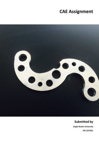
23
Workbook Part B:
Given to us
An Aluminium plate with predrilled holes.
Diameter of both the holes
d1 & d2 = Ø = 11.1
And both the holes are 100 mm apart from the center each.
Thickness of the Aluminium plate = 6 mm
A mandatory hole of 12 mm Ø has to be created in the center of distance between both predrilled holes, at any point (refer Figure)
To Obtain
To obtain an final product either in ‘S’ or ‘V’ shape as a part of design restriction, that needs to be trimed out of this Aluminium plate.
The Part is subjected to the following conditions:
Force = 450 N applied to one pre drilled hole.
Displacement applied top the other end.
Safety Factor of at least 2
Displacement to be greater than 0.2mm but in between 0.23 & 1.2 mm
Figure 30 Dimension

24
Methodology:
The design of the part follows a very simple procedure. The idea is generated to follow an ‘S’ shape for the final design. However
from idea to sketch and physical part takes multiple steps including Inventor, Ansys workbench and Autodesk Inventor.
The first step was to basic design (aluminium plate) with the mentioned specifications (refer Autodesk steps page ). The basic
aluminium block is analysed in Ansys to observe the physical properties before proceedings for any iterations for the final product.
The stress for the material is calculated from a predefined data obtained from an observation. A set of forces is given and the area
could be calculated from the given length and breath which is 31.86mm2
. (refer figure ) (Refer Appendix for the calculation)
Stress graph is generated. Following the graph where the yield point starts to generate is 130 MPa (refer figure ) . This is later
considered for the Ansys’s Work bench simulation while changing the engineering data.
Figure 31 General graph to calculate the Stress at a point
The iterations are made in the inventor. Consecutive three nearest iterations are picked for analysis to reach to the final design. Each
iteration is then analyzed on the ANSYS workbench for the best matched results. Using CAM the code for the final product is
generate for manufacturing. The final step is the physical testing of the product and comparing the results with FEA.
mm
MPa

25
Inventor Design:
Base Design:
The base plate is designed with the predrilled holes and the hole is the centre (figure 32). On a plane, a rectangle This is later
analysed in the ANSYS to find the basic stress by applying force and displacement in the holes*(1)
(figure ). The engineering values are
updated in the ANSYS (figure ). The calculated Tensile and yield stress is 134 MPa which is fed.
Figure 32 Inventor Design and 3D representation
On the application of force and fixed boundaries in figure, it gave a clear approach of structuring the S shape & the place how to
remove the excess metals.
* Holes have been split in inventor, since application of force & displacement is just on one half of the hole not on the entire.
Figure 33 Deformation detailed on simulation in Ansys
Figure 34 Stress in ANSYS for the plate

26
Iteration 1
The first iteration was a rough cut made out of the base plate. It was a basic S shaped model. The 3D model was finished in inventor
and analysed in Ansys, with the same boundary conditions. The modified engineering data and value were kept mentioned in Base
Design
Figure 35 1st iteration S shape model.
Figure 36 Ansys boundary conditions application
Figure 37 Stress

27
Figure 38 Deformation in the body
Result:
The result was clear. The model failed to achieve the required criteria. However the Ansys Analysis provided valuable feedback of the
regions shown in blue with least deformation and minimal stress levels. This was keenly observed & focused for design alteration in
next iteration.

28
Iteration 2
The feedback from the iteration 1 was incorporated in this model. This focused on regions which reacted least in deformation on the
application of force. Since the previous model, this was way lighter, specific with more deformation.
Figure 39 2nd Iteration
Figure 40 Ansys loading & boundary Conditions

29
Figure 41 Stress
Figure 42 Deformation

30
Result:
From the data obtained on running Ansys static loading simulation, the part met the deformation and the safety factor however
failed in achieving lesser stress requirements.
Stress: Regions of high stress concentrations are visible in the red region around the holes. (Refer Fig. 41).
Deformation: The deformation was acceptable with large patch in blue region which could have been removed to lesser the weight
and obtain more deformation. (Refer Fig, 42)
Meshing: Finite element size was selected. Three layers of mesh with 2mm element size.

31
Iteration 3
The iteration focused on obtaining the required minimal stress in ANSYS simulation with addition to removing mass and making the
product lighter in weight though adding more mass near the holes as those regions suffered high stress concentration. The pre
design was altered in inventor.
Figure 44 3rd iteration in inventor.
Figure 45 Boundary Conditions

32
Figure 46 Stress

33
Result:
The model succeeded in achieving the requirements. Design alterations included removal of more mass around the edges and
generation of 4 holes with 9 mm dimensions and 2 holes with 6 mm diameter. This helped in achieving the least weight till so far.
Stress: Clearly the part passed the requirement. The maximum stress was 64.3 MPa around the red region near the displacement (fig
46)
Deformation: The part achieved a deformation of maximum 0.20 mm
Safety Factor: The safety factor achieved was 2.004 which is acceptable.
However due to ergonomics and deign safety, it is unacceptable to have sharp edges. This also included that edges of the part
couldn’t have hollow holes as this would create complexity in the design.

34
Final Part
The final part is exactly the same as the previous iteration (Numbered 3). This was modified to have solid edge with least circular
sharp edges and make the design to be more ergonomic.
Figure 49 Final Design Inventor
Figure 50 Boundary Conditions
Figure 51 Meshing at 7 mm

35
Figure 52 Skweness at 7mm
Meshing Analysis
Figure 53 Aspect ratio in meshing and percentage below
Aspect Ratio
It is important to have a fine size of meshing for the accuracy of the part results. Meshing results vary the accuracy of the model.
With a mesh size of 2mm, the researcher has obtained 3 layers of mesh on the surface of the model. Ideal three layers of mesh
achieves correct reactions to the boundary conditions.
From the figure 98.96% of the mesh elements lie in the region of 1.04 which is nearer to one compared to the mesh size of 7 mm in
figure 52.

36
Skweness
The tendency of the element size which can be as close to the exact geometrical shapes. Higher the Skweness results in absurd
results which effects the stress analysis. It can be seen in the figure that the Skweness for 20% of the elements lie in the region of
0.01 while 34.90% in 0.13. This means the tendency is approximately in region of fractional difference. Hence it can considered as
reason good Skweness
Element Quality

37
Figure 54 Elements in 2 mm showing the fine percentage of element quality
With 2mm mesh sizing , almost 59.81% of the elements lie in the region of 1 while very few or approximately 38% lie in the region of
0.88 which is close to the accuracy of 1. Hence it can considered as a very fine mesh quality.

38
Figure 55 Element Quality in selected elements
Figure 56 Selected element quality

39
Figure 57 Stress in final model
Figure 58 Stress changing (Red region)
Figure 59 Final Stress in the red region from simulation

40
Result:
The model was considered to be a pass after the simulation FEA tests in Ansys. The model met the criteria of the design specification
Stress achieved on the part with 2 mm fine meshing resulted in a concentrated region with 64.08MPa however almost 1/3rd
of the
part seemed to have stress varying from 14.48 MPa to 35.74 MPa
Deformation achieved is 0.21 which is acceptable
Safety Factor obtained from the Ansys results is 2.1 which also satisfied the criteria.

41
Manufacturing Model - CNC
The part design is now ready to be manufactured. As in engineering, any design drawn in a software is coded in binary language for
CNC machines. Machines do not understand values in terms of English language. This is done by converting the data into binary
language of 0’s & 1’s. Most of the 2D & 3D sketch designing software comes with built in CAM (Computer Aided Manufacturing).
Auto desk CAM 2014 has been used to manufacture the part.
Steps manufacturing the part:
1. The final part is exported to Inventor CAM 2014
2. Using standard tools available on the toolbar the model is selected from the Aluminium plate
3. Adding fixed dimensions of the part and selecting phase, the model is generated.
4. Fixed holes are drilled first, following the central hole and the additional holes.
5. The part is phased out with rough cut and a final cut milling tools.
This standard steps involved milling, facing and drilling steps. The code generated was later sent to the CNC programmer to
manufacture the part.
For the CNC Code please refer Appendix.
(Refer Anglia Ruskin University, Notes, VLE)
Figure 62 Final Part Front face

42
Figure 63 Final Part back face.

43
Results (Physical Test)
Physical Part
The physical part suffered necking exactly below the 2nd
circle from the left under the impression of increasing stress. The deformation took place at the part of necking,
However the stress was too less to break the metal apart. This confirms elastic behavior of the material under force.
Figure 64 Part developed necking after the physical test.
Area of necking under stress.
Application of Displacement
Application of force.

44
Zoomed view of the necking
Figure 65 Zoom view

45
Testing
Once the part is clamped in fixed displacement, force is applied slowly from the top hole (figure ) in constant time intervals of 5 secs.
The values of the deformation and force applied is fed in the computer.
Figure 66 Tensile Stress
The testing machine is called Hounsfield Tensile Tester a Tensometer. The device generates the tensile strength of the materials and
the young’s modulus.

46
Figure 67 Time interval graphs with force and deformation
The graph obtained is shown below.
This represents the Stress ratio deformation which is axial movement. From the graph the maximum force obtained is 1200.
Therefore to obtain the safety factor, it can derived as
Total Stress / Total Force ie. 1200/ 450 = 2.66
Stress
Deformation
Necking point

47
Validation
The results obtained from Ansys and the physical tests are in coherence. On maximum Force of 450 N the part starts to generate
necking around the region shown below which is similar to the region displayed in Ansys.
Figure 68 Comparision picture between physical part & Ansys
Exact location of the stress concentration showing the similar result obtained in Part Physical test & Ansys simulation.
The safety factor achieved in Ansys is 2.1 while the physical test records show the safety factor achieved is 2.66 which very closely
similar result obtained in Ansys.
Other the other hand Ansys displayed least deformation stress levels in the other regions which is exactly similar to the part as no
other deformation region can be seen.
Hence we conclude that our test results are validated with the Ansys results obtained.

48
Conclusion
With the above experiments and practical hands on the software, it can be well said that FEA is a vital aspect of engineering. Things
can be researched and analysed in instances. Ansys Workbench as a CAE and FEA software has a crucial role in understanding any
design. Since the research report focused on the static analysis, it can be well versed that every engineering design that is cored into
a final product for market undergoes vivid test. As physically these tests are time consuming & tiring. Ansys Workbench resolves the
problem in fraction of seconds. Individual parts and local meshing can be solved by Ansys.
One of the interesting fact that was observed during this research was the workbench offered multiple material selection with ability
to change their physical properties like tensile strength & much more.
Not only the simulations showed a concentrated analysis of the material behaviour but the exact results of the physical test.
In nut it can be summarised, CAE is not only mere a part of R&D but plays a core role in concurrent engineering with easy and
standard approach to the problem.

49
References
Inc., A. (2014, November 1st). ANSYS Workbench. Retrieved from ANSYS : http://www.ansys.com/en_uk
Lee, H. -H. (2011). Ansys Workbench 13 . Stephen Schroff.
Siemens. (2014, November 4th ). Siemens PLM software. Retrieved from Siemens FEA software:
http://www.plm.automation.siemens.com/en_gb/plm/fea.shtml

1
1
2
2
3
3
4
4
A A
B B
C C
D D
SHEET 1 OF 1
DRAWN
CHECKED
QA
MFG
APPROVED
dl411 05/01/2015
DWG NO
TITLE
SIZE
C
SCALE
REV
R36.98
11.109.00
9.00
6.00
9.00
12.00
6.00
R5.55
R10.59
R13.97
R6.00
R27.92
R36.98
6.47
R10.59
100.00
R36.96
R13.34
R36.96
1227201 CAE Part
Aluminium part for tensile test
1227201
2:1

An Advanced learning FEA, CAE - Ansys, Inventor CAM

Recommended

Recommended

More Related Content

What's hot

What's hot (20)

Viewers also liked

Viewers also liked (11)

Similar to An Advanced learning FEA, CAE - Ansys, Inventor CAM

Similar to An Advanced learning FEA, CAE - Ansys, Inventor CAM (20)

Recently uploaded

Recently uploaded (20)

An Advanced learning FEA, CAE - Ansys, Inventor CAM