
Recommended
Recommended
More Related Content
What's hot
What's hot (20)
Similar to Vogel’s Approximation Method (VAM)
Similar to Vogel’s Approximation Method (VAM) (20)
Recently uploaded
Recently uploaded (20)
Vogel’s Approximation Method (VAM)
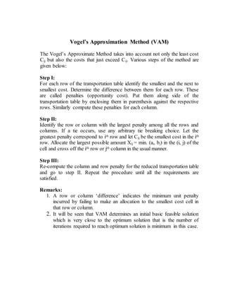
- 1. Vogel’s Approximation Method (VAM) The Vogel’s Approximate Method takes into account not only the least cost Cij but also the costs that just exceed Cij. Various steps of the method are given below: Step I: For each row of the transportation table identify the smallest and the next to smallest cost. Determine the difference between them for each row. These are called penalties (opportunity cost). Put them along side of the transportation table by enclosing them in parenthesis against the respective rows. Similarly compute these penalties for each column. Step II: Identify the row or column with the largest penalty among all the rows and columns. If a tie occurs, use any arbitrary tie breaking choice. Let the greatest penalty correspond to ith row and let Cij be the smallest cost in the ith row. Allocate the largest possible amount Xij = min. (ai, bj) in the (i, j) of the cell and cross off the ith row or jth column in the usual manner. Step III: Re-compute the column and row penalty for the reduced transportation table and go to step II. Repeat the procedure until all the requirements are satisfied. Remarks: 1. A row or column ‘difference’ indicates the minimum unit penalty incurred by failing to make an allocation to the smallest cost cell in that row or column. 2. It will be seen that VAM determines an initial basic feasible solution which is very close to the optimum solution that is the number of iterations required to reach optimum solution is minimum in this case.
- 2. Examples: 1. Balanced Transportation Problem SupplyP Q R S A 18 21 12 15016 B 17 14 13 16019 C 32 11 10 9015 Demand 140 120 90 50 400 Solution: In this example, Total Supply = Total Demand. So, this is balanced transportation problem. P Q R S Supply Penalities A 18 21 12 150 416 B 17 14 13 160 119 C 32 11 10 90 115 Demand 140 120 90 50 400 Penalities 1 7 1 2 For each row and column of the transportation table determine the penalties and put them along side of the transportation table by enclosing them in parenthesis against the respective rows and beneath the corresponding columns.
- 3. Select the row or column with the largest penalty i.e. (7) (marked with an arrow) associated with second column and allocate the maximum possible amount to the cell (3,2) with minimum cost and allocate an amount X32=Min(120,90)=90 to it. This exhausts the supply of C. Therefore, cross off third row. The first reduced penalty table will be: Supply PenalitiesP Q R S A 18 21 12 150 416 B 17 14 13 160 119 Demand 140 30 90 50 310 Penalities 1 1 7 1 In the first reduced penalty table the maximum penalty of rows and columns occurs in column 3, allocate the maximum possible amount to the cell (2,3) with minimum cost and allocate an amount X23=Min(90,160)=90 to it . This exhausts the demand of R .As such cross off third column to get second reduced penalty table as given below. Supply PenalitiesP Q S A 18 12 150 416 B 17 19 13 160 4 191 919 Demand 140 30 50 220 Penalities 1 1 1 In the second reduced penalty table there is a tie in the maximum penalty between first and second row. Choose the first row and allocate the maximum possible amount to the cell (1,4) with minimum cost and allocate an amount
- 4. X14=Min(50,150)=50 to it . This exhausts the demand of S so cross off fourth column to get third reduced penalty table as given below: Supply PenalitiesP Q A 18 100 216 B 17 19 70 2 191 919 Demand 140 30 170 Penalities 1 1 The largest of the penalty in the third reduced penalty table is (2) and is associated with first row and second row. We choose the first row arbitrarily whose min. cost is C11 = 16. The fourth allocation of X11=min. (140, 100) =100 is made in cell (1, 1). Cross off the first row. In the fourth reduced penalty table i.e. second row, minimum cost occurs in cell (2,1) followed by cell (2,2) hence allocate X21=40 and X22=30. Hence the whole allocation is as under: SupplyP Q R S A 100 18 21 50 12 150 16 B 40 30 90 14 13 160 17 19 C 32 90 11 10 90 15 Demand 140 120 90 50 400 The transportation costaccording to the above allocation is given by Z = 16 × 100 + 12 × 50 + 17 × 40 +19 × 30 + 14 × 90 + 11 × 90 = 5700
- 5. 2. Unbalanced Transportation Problem A B C Supply P 4 8 8 76 Q 16 24 16 82 R 8 16 24 77 Demand 72 102 41 Solution: In this example, Total Supply is 235 and Total Demand is 225. Here Total Supply > Total Demand. So, this is unbalanced transportation problem. To solve this problem we need to make it balanced transportation problem. Here we introduce dummy column with transportation cost including the dummy. Thus new balanced transportation table is as: A B C Dummy Supply P 4 8 8 0 76 Q 16 24 16 0 82 R 8 16 24 0 77 Demand 72 102 41 200
- 6. A B C Dummy Supply Penalities P 4 8 8 0 76 4 Q 16 24 16 0 82 16 R 8 16 24 0 77 8 Demand 72 102 41 20 Penalities 4 8 8 For each row and column of the transportation table determine the penalties and put them along side of the transportation table by enclosing them in parenthesis against the respective rows and beneath the corresponding columns. Select the row or column with the largest penalty i.e. (16) (marked with an arrow) associated with second row and allocate the maximum possible amount to the cell (2,4) with minimum cost and allocate an amount X24=Min(20,82)=20 to it. This exhausts the demand of dummy. Therefore, cross off forth column. The first reduced penalty table will be: A B C Supply Penalities P 4 8 8 76 4 Q 16 24 16 62 8 R 8 16 24 77 8 Demand 72 102 41 Penalities 4 8 8
- 7. In the first reduced penalty table there is a tie in the maximum penalty between second row, third row, second column and third column . Choose the second column and allocate the maximum possible amount to the cell (1,2) with minimum cost and allocate an amount X12=Min(102,76)=76 to it . This exhausts the supply of B so cross off first row to get second reduced penalty table as given below: A B C Supply Penalities Q 16 24 16 82 8 R 8 16 24 77 8 Demand 72 26 41 Penalities 8 8 8 In the second reduced penalty table there is a tie in the maximum penalty between all rows and columns. Choose the first column and allocate the maximum possible amount to the cell (2,2) with minimum cost and allocate an amount X12=Min(72,77)=72 to it . This exhausts the demand of A so cross off first column to get third reduced penalty table as given below: B C Supply Penalities Q 24 16 82 8 R 16 24 5 8 Demand 102 41 Penalities 8 8
- 8. In the third reduced penalty table there is a tie in the maximum penalty between all rows and columns. Choose the first column and allocate the maximum possible amount to the cell (1,2) with minimum cost and allocate an amount X12=Min(41,82)=41 to it . This exhausts the demand of C so cross off second column to get fourth reduced penalty table. In the fourth reduced penalty table i.e. second row, minimum cost occurs in cell (2,1) followed by cell (1,1) hence allocate X21=5 and X22=21. Hence the whole allocation is as under: A B C Dummy Supply P 4 76 8 8 0 76 Q 16 21 41 16 20 0 82 24 R 72 5 16 24 0 77 8 Demand 72 102 41 20 The transportation costaccording to the above allocation is given by Z = 8 × 76 + 24 × 21 + 16× 41 + 0 × 20 + 8 × 72 + 16 × 5 = 2424