book chapter ; Quantum technology, quantum computing, quantum sensing, quantum cryptography

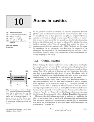
1. 10
10.1 Optical cavities 194
10.2 Atom–cavity coupling 197
10.3 Weak coupling 200
10.4 Strong coupling 206
10.5 Applications of cavity
effects 211
Further reading 213
Exercises 214
Atoms in cavities
In the previous chapter we studied the resonant interaction between
photons and an atomic transition of the same frequency. The atoms
we considered were in free space and the photons originated from an
external source such as a lamp or laser beam. We now wish to re-explore
this process in more detail for the special case in which the interaction
between the photons and the atom is enhanced by placing the atom
inside a resonant cavity. This will naturally lead us into the subject of
cavity quantum electrodynamics (cavity QED). We begin our discussion
by considering the key parameters that determine the properties of the
cavity and the magnitude of the atom–cavity coupling, and then explore
the different physical effects that are observed in the limits of weak and
strong coupling to the cavity.
10.1 Optical cavities
Before studying the interaction between atoms and cavities, it is helpful
to remind ourselves of some of the basic properties of optical cavities.
We shall restrict our attention here to the simplest case, namely a planar
cavity. This will be sufficient to illustrate the chief points, and the results
can then be generalized to other types of cavity. The planar cavity is
covered in detail in most classical optics texts, and we give here only a
brief summary of the results that are relevant to our discussion.
Fig. 10.1 A planar cavity of length
Lcav with two parallel end mirrors M1
and M2 of reflectivity R1 and R2,
respectively. The medium inside the
cavity has a refractive index n. The
cavity acts as a Fabry–Perot inter-
ferometer when light of wavelength λ
is introduced through one of the end
mirrors.
Consider the planar cavity shown in Fig. 10.1. The cavity consists of
two plane mirrors M1 and M2, with reflectivities of R1 and R2, respect-
ively, separated by an adjustable length Lcav. The space between the
mirrors is filled with a medium of refractive index n and the mirrors
are aligned parallel to each other so that light inside the cavity bounces
backwards and forwards between the mirrors. Planar cavities of the type
shown in Fig. 10.1 are frequently used in high-resolution spectroscopy,
in which case the instrument is called a Fabry–Perot interferometer.
The properties of the planar cavity can be analysed by considering the
effect of introducing light of wavelength λ from one side and calculating
how much gets transmitted through to the other side. On the assumption
that there are no absorption or scattering losses within the cavity, the
transmission T is given by:
See, for example, Brooker (2003), Hecht
(2002), or Yariv (1997).
T =
1
1 + (4F2/π2) sin2
(φ/2)
(10.1)

2. 10.1 Optical cavities 195
where
φ =
4πnLcav
λ
(10.2)
is the round-trip phase shift, and
F =
π(R1R2)1/4
1 −
√
R1R2
(10.3)
is the finesse of the cavity. It is easy to see from eqn 10.1 that the
transmission is equal to unity whenever φ = 2πm, where m is an integer.
In this situation the cavity is said to be on-resonance. From eqn 10.2
we see that the resonance condition occurs when the cavity length Lcav
is equal to an integer number m of intracavity half wavelengths:
Lcav = mλ/2n. (10.4)
The resonance condition thus occurs when the light bouncing around
the cavity is in phase during each round trip.
Fig. 10.2 Transmission of a lossless
planar cavity with mirror reflectivities
of 90%, giving a finesse F of 30. Reso-
nance occurs whenever the round-trip
phase equals 2πm, where m is an
integer.
Figure 10.2 shows the transmission of a lossless planar cavity with
R1 = R2 = 0.9, giving F = 30. The transmission is a sharply peaked
function of the round-trip phase shift φ, with maxima at the resonance
values of φ = 2πm. The width of the peaks can be calculated by find-
ing the condition for T = 50%. In the limit of large F, this is easily
calculated from eqn 10.1 and gives
φ = 2πm ± π/F. (10.5)
The full width at half maximum (FWHM) is therefore equal to
ΔφFWHM = 2π/F, (10.6)
which implies: The cavity finesse is usually defined
as the ratio of the separation of adja-
cent maxima to the half width, as in
eqn 10.7.
F =
2π
ΔφFWHM
. (10.7)
The finesse of the cavity determines the resolving power when using the
instrument for high-resolution spectroscopy.
The cavity resonance condition naturally leads to the concept of
resonant modes. These are modes of the light field that satisfy the
resonance condition and are preferentially selected by the cavity. Since
the light fields bouncing around the cavity are all in phase, the waves
interfere constructively and have much larger amplitudes than at non-
resonant frequencies. The resonant modes have intensities inside the
cavity enhanced by a factor 4/(1 − R) compared to an incoming wave,
while the out of resonance frequencies have their intensity suppressed
by a factor (1 − R). (See Exercise 10.2.) The properties of the resonant
modes play an essential part in determining the emission spectra of
lasers, and will also be very important for the discussion of the emission
properties of atoms in cavities.
The angular frequencies of the resonant modes are easily worked out
from eqn 10.4 and are given by:
ωm = m
πc
nLcav
. (10.8)

3. 196 Atoms in cavities
The mode frequencies can be tuned either by changing Lcav or n. Since
the mode frequency is proportional to the phase, we can use eqn 10.7 to
relate the spectral width Δω of the resonant modes to the properties of
the cavity:
Δω
ωm − ωm−1
=
ΔφFWHM
2π
=
1
F
, (10.9)
giving:
The cavity length is typically tuned by
moving one of the mirrors with a piezo-
electric transducer. The method used
for tuning the refractive index depends
on whether the cavity is filled with
a gas or a solid. In the former case,
the refractive index can be controlled
through the gas pressure, and in the
latter, by heating the cavity and using
the temperature dependence of n.
Δω =
πc
nFLcav
. (10.10)
This shows that cavities with high finesse values have sharp resonant
modes.
The final quantity that we need to consider is the photon lifetime
τcav inside the cavity. Consider a light source at the centre of a sym-
metric, high-finesse cavity with R1 = R2 ≡ R ≈ 1. We suppose that the
source emits a short pulse of light containing N photons into the cavity
mode at time t = 0 as shown in Fig. 10.3. We assume that the fractional
photon number change at each reflection is small due to the high reflec-
tivity of the mirrors. After a time t = nLcav/c, the pulse will have gone
around half the cavity, and the photon number will be equal to RN. At
t = 2nLcav/c, the pulse will have completed a round trip and the pho-
ton number will be equal to R2
N. This process continues until all the
photons are lost from the cavity. On average, we lose ΔN = (1 − R)N
photons in a time equal to nLcav/c. We can therefore write:
dN
dt
= −
ΔN
nLcav/c
= −
c(1 − R)
nLcav
N, (10.11)
which has solution N = N0 exp(−t/τcav), where the photon lifetime is
given by:
τcav =
nLcav
c(1 − R)
. (10.12)
It is helpful to define the photon decay rate (κ) as:
κ =
1
τcav
. (10.13)
Fig. 10.3 Decay of the cavity photon number following emission from a pulsed source
at the centre of the cavity at t = 0. The mirror reflectivities are assumed to be high,
so that the fractional loss per round trip is small.

4. 10.2 Atom–cavity coupling 197
We can then combine eqns 10.3, 10.10, and 10.12 with R ≈ 1 to find:
Δω = (τcav)−1
≡ κ. (10.14)
This shows that the width of the resonant modes is controlled by the
photon loss rate in the cavity, in exactly the same way that the natu-
ral width of an atomic emission line is controlled by the spontaneous
emission rate (cf. eqn 4.30).
The analysis of the linear cavity shows that there are basically two
key parameters that determine the main properties, namely the reso-
nant mode frequency ωm and the cavity finesse F. The latter parameter
controls both the mode width Δω and the cavity loss rate κ. In dealing
with other types of cavity it is helpful to introduce the quality factor
(Q) of the cavity, defined by:
Q =
ω
Δω
. (10.15)
This serves the equivalent purpose for a general cavity as the finesse
does for the planar cavity. It is thus convenient to specify the properties
of a cavity either by the frequency and finesse, or equivalently by the
frequency and quality factor.
Fig. 10.4 A two-level atom in a reso-
nant cavity with modal volume V0. The
cavity is described by three parame-
ters: g0, κ, and γ which, respectively
quantify the atom–cavity coupling, the
photon decay rate from the cavity, and
the non-resonant decay rate. Note that
the cavity in Fig. 10.4 is drawn with
concave mirrors rather than plane ones.
If the cavity only had plane mirrors,
then off-axis photons emitted by the
atom would never re-interact with it.
The use of concave mirrors reduces this
problem.
10.2 Atom–cavity coupling
Having reminded ourselves of the relevant properties of optical cavities,
we can now start to discuss the interaction between the light inside a
cavity and an atom, as shown schematically in Fig. 10.4. We assume that
the atom is inserted in such a way that it can absorb photons from the
cavity modes and also emit photons into the cavity by radiative emission.
We are particularly interested in the case where the transition frequency
of the atom coincides with one of the resonant modes of the cavity. In
these circumstances, we can expect that the interaction between the
atom and the light field will be strongly affected, since the atom and
cavity can exchange photons in a resonant way.
The transition frequencies of the atom are determined by its internal
structure and are taken as fixed in this analysis. The resonance condition
is then achieved by tuning the cavity so that the frequency of one of the
cavity modes coincides with that of the transition. At resonance we find
that the relative strength of the atom–cavity interaction is determined
by three parameters:
• the photon decay rate of the cavity κ,
• the non-resonant decay rate γ,
• the atom–photon coupling parameter g0.
These three parameters each define a characteristic time-scale for the
dynamics of the atom–photon system. The interaction is said to be in
the strong coupling limit when g0 (κ, γ), where (κ, γ) represents the
larger of κ and γ. Conversely, we have weak coupling when g0 (κ, γ).