SlideShare a Scribd company logo
1 of 45
Observed Climate–Snowpack Relationships in California and
their
Implications for the Future
SARAH KAPNICK AND ALEX HALL
University of California, Los Angeles, Los Angeles, California
(Manuscript received 27 October 2008, in final form 11
December 2009)
ABSTRACT
A study of the California Sierra Nevada snowpack has been
conducted using snow station observations and
reanalysis surface temperature data. Monthly snow water
equivalent (SWE) measurements were combined
from two datasets to provide sufficient data from 1930 to 2008.
The monthly snapshots are used to calculate
peak snow mass timing for each snow season. Since 1930, there
has been an overall trend toward earlier snow
mass peak timing by 0.6 days per decade. The trend toward
earlier timing also occurs at nearly all individual
stations. Even stations showing an increase in 1 April SWE
exhibit the trend toward earlier timing, indicating
that enhanced melting is occurring at nearly all stations.
Analysis of individual years and stations reveals that
warm daily maximum temperatures averaged over March and
April are associated with earlier snow mass
peak timing for all spatial and temporal scales included in the
dataset. The influence is particularly pro-
nounced for low accumulation years indicating the potential
importance of albedo feedback for the melting of
shallow snow. The robustness of the early spring temperature
influence on peak timing suggests the trend
toward earlier peak timing is attributable to the simultaneous
warming trend (0.18C decade
21
since 1930, with
an acceleration in warming in later time periods). Given future
scenarios of warming in California, one can
expect acceleration in the trend toward earlier peak timing; this
will reduce the warm season storage capacity
of the California snowpack.
1. Introduction
The California water supply is determined by cold
season precipitation (rain in low elevations and snow in
high elevations) and the capacity of natural and man-
made reservoirs. Most manmade reservoirs were built in
the early twentieth century for two purposes: 1) the
storage and disbursement of cold season rains and 2) the
storage and disbursement of runoff from spring snow-
melt. Reservoirs were designed to store only a fraction
of the state’s total yearly precipitation, under the as-
sumption that a sufficient delay between winter rains
and spring snowmelt runoff would always exist, with
snowmelt occurring at roughly the same time every year.
The annual mountain snowpack thus provides natural
storage for the water supply until the onset of snowmelt.
Changes in the amount of precipitation, percentage of
precipitation falling as rain instead of snow, and onset of
snowmelt can therefore affect the state’s water supply.
During anomalously high rain or snowmelt events, res-
ervoirs must not only store water, but also discharge
excess water to avoid flooding. Water must sometimes
even be discharged in anticipation of large events to re-
duce flood risk. The dual functions of storage and flood
management require reservoir managers to carefully
balance factors such as precipitation, snowmelt timing,
reservoir storage capacity, and demand. Even if future
climatological precipitation remains unchanged, shifts
in snowmelt timing can affect California’s water supply
during the warm season because of reservoir storage ca-
pacity constraints. To understand changes in snowmelt
water supply as a result of climate change, it is therefore
important to understand changes in the timing of snow-
melt in addition to total spring snowpack amounts.
Snowpack measurements are essential for predicting
timing and amount of warm season snowmelt runoff. For
this reason, a network of stations in the western United
States dating back to the 1930s tracks water content of
snow (also known as snow water equivalent; SWE). Mea-
surements are taken manually around the first of the
month at each station according to a prescribed monthly
Corresponding author address: Sarah Kapnick, University of
California, Los Angeles, P.O. Box 951565, Los Angeles, CA
90095-
1565.
E-mail: [email protected]
3446 J O U R N A L O F C L I M A T E VOLUME 23
DOI: 10.1175/2010JCLI2903.1
� 2010 American Meteorological Society
schedule. Because of the desire to track peak SWE—
thought to occur in early April—many more records are
available on or around 1 April (Serreze et al. 1999). Pre-
vious snowpack studies have focused on this well-sampled
1 April SWE dataset (Barnett et al. 2008; Mote 2006; Mote
et al. 2005; Cayan 1996) to assess the climatology and
variability of snowpack in the western United States.
These studies are important for understanding total melt-
water available during the warm months, but do not
directly address the timing of the transition from accu-
mulation to melt from snow observations.
Ideally, high-temporal resolution data would be avail-
able to study the evolution of the snowpack over the
course of the season, particularly the exact date and
amount of maximum SWE and subsequent melt rates.
Stations have been built in California since the 1970s
to measure daily SWE automatically, but do not begin
early enough for long-term variability analysis. Previous
observational studies have instead utilized streamflow
data, presumably snowmelt-dominated, as a proxy for
snowmelt timing. They show there has been a trend in
streamflow discharge toward earlier in the spring using
a variety of streamflow metrics (Regonda et al. 2005;
Stewart et al. 2005; Cayan et al. 2001). Daily SWE data
from 1992 to 2002 has also been combined with long-
term historic streamflow data to study the onset of
spring in the Sierra Nevada (Lundquist et al. 2004);
however, because of the shortness of the SWE time
series, streamflow measurements must still be relied
upon to measure long-term variability in snowmelt.
Unfortunately, this indirect variable is not a perfect mea-
sure of snowmelt, as it can be influenced by other factors
such as precipitation, temperature, lithology, soil compo-
sition, vegetation (Aguado et al. 1992), and presnowmelt
soil moisture.
Modeling studies to produce SWE, temperature, and
precipitation values have also been conducted to assess
changes in the snowpack of the Western United States.
Hamlet et al. (2005) created a snowpack simulation from
1915 to 2003 using the variable infiltration capacity hy-
drologic model as a surrogate for historical SWE ob-
servations and found that downward trends in 1 April
SWE and trends toward earlier peak snow accumulation
were due to warming over the period. Pierce et al. (2008)
produced simulations for 1600 years using two global
circulation models, yielding evidence that SWE as a per-
centage of precipitation has had a negative trend because
of anthropogenic forcing that will continue in the future.
These modeling studies show that the Sierra snowpack
has been declining and project a continuance of a nega-
tive trend in SWE in the future.
To study changes in the California snowpack directly
and provide a purely empirical sensitivity for future
projections, the present study focuses on observations of
monthly SWE. A dataset has been compiled from two
different sources to provide sufficient stations with SWE
measurements from mid-January through mid-May over
a long enough time period to do robust trend and sen-
sitivity analysis. The monthly data is used to infer peak
snow mass timing from February to May. Over this re-
cord stretching roughly from 1930 to the present, the
peak timing exhibits a trend toward earlier in the season.
Much of this trend can be explained by the sensitivity
of snow mass peak timing to early spring temperature.
Given future warming scenarios in the California Sierra
Nevada, we conclude the trend in earlier peak timing
will continue.
2. Data
A snow station dataset was compiled from two exist-
ing datasets for the state of California: the National
Resources Conservation Service (NRCS) and Water and
Climate Center (www.wcc.nrcs.usda.gov/snowcourse/) and
the California Department of Water Resources (http://
cdec.water.ca.gov/misc/SnowCourses.html). A total of
154 stations across California with recorded SWE data
from mid-January to mid-May with at least 30 years of
data from 1930 to 2008 are used (see Fig. 1). These
stations range in their years of available data. We show
that these temporal gaps have a negligible impact on our
analysis in the appendix. It has been noted that the exact
timing of historical monthly snow course measurements
can vary, with some measurements being taken within
a few days of the first-of-the-month measurement date
(Cayan 1996). In these measurements, there may also be
a systematic shift in the actual date of measurement
toward later (Mote et al. 2005). To circumvent these
issues we only selected stations with exact measurement
dates corresponding to raw SWE data for our analysis.
The correlations shown in this paper are noticeably re-
duced when SWE values are assumed to be first-of-the-
month values; such employment of SWE measurements
may therefore lead to a nonnegligible source of random
error in the other studies. Subsequent sections will de-
scribe criteria used to produce subsets of data for analysis.
Temperature data are also used to diagnose snow
accumulation and melt processes. Maximum and mini-
mum daily temperature data from 1930 to 2003 were
obtained from the Surface Water Modeling group at the
University of Washington from their Web site (www.hydro.
washington.edu/Lettenmaier/Data/gridded/) the develop-
ment of which is described by Hamlet and Lettenmaier
(2005). This dataset was chosen for its long temporal
coverage (1915–2003) and high spatial resolution (1/ 88)
relative to other pre-satellite-era temperature products.
1 JULY 2010 K A P N I C K A N D H A L L 3447
This product has also been used in previous snowpack
studies (Mote et al. 2005; Hamlet et al. 2005).
3. Methods and results
a. Calculation of snow mass peak
To assess interannual variations in California snow-
pack evolution, a metric was developed quantifying sys-
tematic changes in snow accumulation and melt timing.
In particular, we focused on the timing of peak snow
mass. We created a measure of this quantity relying on
SWE measurements taken around the first-of-the-month
from February to May. We used these monthly snap-
shots rather than daily SWE data because the daily data
are only robustly available from 1980 to the present, too
short a time series to calculate long-term trends in max-
imum SWE timing.
The peak snow mass timing is defined for any given
year as the temporal centroid date, also known as the center
of mass, of SWE values (SWE centroid date; SCD) from
approximately 1 February to 1 May for stations with
complete data over this four-month time period. The
SCD is given by the equation:
SCD 5
� t
i
SWE
i
�SWE
i
. (1)
Each individual measurement during the season is dis-
tinguished by i. The SWE measurements are given by
SWEi in centimeters. The value ti is the exact date of the
measurement in Julian days and falls within two weeks
of the first of the month for February, March, April, and
May. The SCD metric is similar to that used in previous
studies of streamflow peak timing (Stewart et al. 2004,
2005). Figure 2a provides a visualization of this calcu-
lation for a location and a year when daily data are also
available. As is clear from the figure, SCD captures the
gross timing of snow processes. For the peak to shift earlier
FIG. 1. Location of 154 snow stations with usable data in
California. Open circles denote
NRCS Water and Climate Center stations and closed circles
denote California Department of
Water Resources stations. Stations are colored by elevation in
meters.
3448 J O U R N A L O F C L I M A T E VOLUME 23
(later), the percentage of snow accumulation later in the
season must decrease (increase), or there must be an in-
crease (decrease) in the percentage of snow melting later
in the season. Thus it corresponds roughly with the peak
in snow mass.
The SCD metric provides a more accurate represen-
tation of the timing of snow accumulation and melt than
the date of absolute maximum SWE value given in the
four approximate first-of-the-month point measurements.
It allows for the snow mass peak timing to shift on the
order of days instead of being constrained to shifts in
monthly increments. Long-term variability in snow mass
peak timing can be studied on submonthly time scales
despite the lack of daily data. As we show below, the
changes in peak snow mass timing in the California Sierra
Nevada are on the order of days, confirming the need for
a metric with this property.
For stations where daily data are available within
close proximity to long-term monthly stations, SCD was
calculated on a daily and monthly basis to assess the
accuracy of using historical monthly SWE values. Daily
SWE values from 15 January to 15 May from 13 stations
were used to calculate a daily SCD, while first-of-the-
month measurements taken from the daily stations were
used to calculate a monthly SCD. These stations were
chosen to correspond to those used in subsequent long-
term monthly trend analysis. For each station, years
missing 10 or more days from January to May were ex-
cluded; this criterion was similarly employed by Knowles
et al. (2006) and developed by Huntington et al. (2004).
The SCD values calculated from monthly and daily data
was found to be extremely highly correlated (r 5 0.98,
p , 0.01), giving confidence that the temporal resolution
of monthly snapshots is high enough to provide accurate
information about snowpack timing.
b. Trends in peak snow mass timing
Examination of SCD from 1930 to 2008 yields evi-
dence that it is trending earlier. When stations with data
for at least 75% of these years are included, SCD is
found to occur earlier at a rate of 0.6 days per decade
(Fig. 3; this is similar to figures showing trends in earlier
spring timing in Cayan et al. (2001)). This trendline has
a slope significantly different than zero (using the Stu-
dent’s t test, p , 0.01). When stations with fewer yearly
SCD values are also included, or when the starting year
of the trendline is set later to include more stations,
statistically significant nonzero trendlines of earlier peak
timing are still found (Table 1). In most cases, the trend
toward earlier peak timing is enhanced (i.e., the trend
becomes more negative). There is a similar enhancement
in the averaged March and April maximum daily tem-
perature warming trend from 1930 to 1970 as successively
FIG. 2. SCD monthly calculation example for (a) one station in
1996 and (b) a comparison of the monthly vs daily
calculations of SCD for 13 stations. In (a), the solid black line
denotes daily 1996 SWE values at the SNOTEL Adin
Mountain station from 1 January to 31 May. The gray bars help
illustrate how four measurements of SWE values are
used to calculate the SCD over the time period shown. The gray
hatch on each bar denotes the first of February,
March, April, and May. The black dashed line at Julian day 72
denotes the SCD found by using the monthly SCD
values. In (b), 13 stations with daily data were used to calculate
SCD using the daily and monthly methods. The
stations were chosen by their proximity to stations used in the
long trend analysis shown in Fig. 3. The monthly
approximation of SCD is well correlated with the daily
calculation of SCD (r 5 0.98, p , 0.01). There are 336 data
points for 13 stations from 1970 to 2008.
1 JULY 2010 K A P N I C K A N D H A L L 3449
later periods of the time series are isolated (Table 1,
last row). We discuss the potential causal link between
the warming and SCD trends in the discussion.
Almost all individual station SCD trends are also neg-
ative (Fig. 4), suggesting a consistent signal from catch-
ment to catchment. In addition, Fig. 4 compares station
trends in SCD to trends in the highly studied 1 April
SWE record. Note that measurements are taken within
two weeks of 1 April for the 1 April SWE record. Mote
et al. (2005) noted that the fluctuation in measurement
date may affect 1 April SWE trends, but concluded that
climatic factors likely have a dominant effect on the trend.
The majority of stations exhibit a negative trend in both
SCD and 1 April SWE. A negative SCD trend is as-
sociated with snow melting earlier, which also results in
trends toward lower SWE. Some of the change in SCD
may also be driven by a shift toward more rain and less
snowfall as described by Knowles et al. (2006); our
analysis shows that only the lowest elevation stations
have exhibited statistically significant trends in both
metrics.
Figure 4 resolves the apparent inconsistency between
increasing 1 April SWE at some locations and a warming
climate. All the points with positive trends in 1 April
SWE have negative trends in SCD. These points all have
positive trends in SWE from February to May (not
shown). Enhanced melting at these locations must there-
fore be compensating for the increased accumulation to
create the negative trend in SCD. The link between
1 April SWE values and melt during previous months
has been observed in some daily Snowpack Telemetry
(SNOTEL) stations in the California Sierra Nevada;
1 April SWE was shown to be highly anticorrelated with
daily melt events from the previous months, implying
changes in 1 April SWE have been due at least in part
to melt events (Mote et al. 2005).
TABLE 1. Trend in peak timing (days decade
21
) for collective
stations and temperature (8C decade
21
) found in the grid cells
covering the snow stations from start date (denoted in columns)
to
2008. Trend in peak timing is given for three different cases: all
stations with available SCD data, stations with data for only
50% of
available years, and stations with data for only 75% of available
years. The SCD trend corresponding to Fig. 3 is given by the
bolded
cell. Trend in average monthly maximum daily temperature at
el-
evations above 1700 m (elevation minimum for snow stations
used
in the bulk of this analysis) is given from start date to 2003
(due to
the limitation of the available temperature dataset) for the
months
of January, February, March, and April with the last row
providing
the averaged March and April temperature trend.
Case 1930 1940 1950 1960 1970
All Stations 20.7 20.8 20.7 20.7 20.4
50% of years 21.0 21.1 20.7 20.7 20.7
75% of years 20.6 20.9 20.8 21.0 20.5
January temperature 0.3 0.3 0.5 0.5 0.7
February temperature 0.2 0.2 0.1 0.0 20.1
March temperature 0.2 0.3 0.4 0.5 0.7
April temperature 0.0 0.1 0.1 0.3 0.5
May temperature 0.1 0.2 0.3 0.3 0.2
Averaged March
and April temperature
0.1 0.2 0.3 0.4 0.6
FIG. 3. SCD for 22 stations with annual data available for at
least 75% of the record from 1930
to 2008. There are 1482 data points for the time period. The
dashed line denotes the mean SCD
(Julian day 76) and the solid line denotes the linear trendline
for the time series.
3450 J O U R N A L O F C L I M A T E VOLUME 23
c. Distribution of peak snow mass timing versus
1 April SWE
Variability in 1 April SWE is evaluated against vari-
ability in the SCD metric to explore relationships be-
tween SCD and the SWE variable used to predict water
supply. Figure 5 shows a scatterplot of 1 April SWE
versus SCD values. Each point represents a snow station
during one snow season. Snow stations with a minimum
of 75% of SCD values over the period from 1950 to 2003
were used for this analysis. This time period was selected
to coincide with the available temperature record and
increase the number of snow stations available for tem-
perature sensitivity studies in section 3d. (A nearly iden-
tical distribution is found if the start date is changed to
1930.) For the given subset of snow stations, SCD occurs
over a wide range, with the average SCD occurring on
Julian day 73 (mid March). The average 1 April SWE
value is 74 cm.
The striking bell-shaped distribution of the 1 April
SWE versus SCD scatterplot arises because of differing
behavior of SCD for large and small seasonal snow
accumulation. When 1 April SWE is large (roughly
$100 cm), the SCD tends to occur in a narrow band
between Julian day 70 and 90, with most points (96%)
above the mean of 73. This corresponds to a time period
mainly falling between the middle of the second and
third bar of Fig. 2, or the calendar month of March. There
are three main reasons for this behavior: 1) To attain
such high 1 April SWE values, relatively consistent storm
activity and steady accumulation is necessary from
February to March. 2) The large accumulation then in-
creases the effective thermal inertia of the snowpack,
delaying the onset of melting. 3) This large accumulation
then only melts once the seasonal warming becomes
great enough to initiate the melting process. These three
processes make for a late SCD, with little variation from
season to season.
When 1 April SWE is small (less than roughly 100 cm)
however, the SCD falls over a large range between
Julian day 21 and 114. This range is more than 4 times
that of the high seasonal accumulation and covers the
middle of the first bar to the middle of the fourth bar
in Fig. 2, or from the last day in January to the end
of April. The significantly greater range in SCD values
is due to two factors: 1) Low accumulation is the re-
sult of a relatively small number of storms with highly
variable timing. 2) Melting in shallow snow is more
sensitive to temperatures above freezing because of
the smaller thermal inertia of shallow snow and its
greater susceptibility to albedo feedback. This results
in earlier (later) snowmelt when temperatures are warm
(cold).
To explore the sensitivity of SCD to temperature fur-
ther, the colorbar given in Fig. 5 distinguishes the distri-
bution of SCD values by local averaged March and April
(MA) maximum daily temperature. The local average
maximum daily temperature for each station is calcu-
lated by taking the local gridcell maximum daily tem-
perature, averaging it over two months, and adjusting it
for the elevation of each station assuming a constant
lapse rate of 6.58C km21. When the distribution of SCD
versus 1 April SWE is distinguished by temperature,
SCD has very little systematic association with either
January or February temperatures, but is closely linked
to early spring temperature (colorbar in Fig. 5). The
correlations of observed SCD and temperatures for dif-
ferent months are shown in the first row of Table 2, and
clearly quantify the influence of late accumulation season
temperature on SCD. Lower MA temperatures appear
to shift SCD into the later half of the season. The most
likely reason for this connection is that snowmelt dur-
ing March and April is reduced (increased) by anoma-
lously cold (warm) March and April temperatures, thus
moving SCD to the later (earlier) portion of the season.
The sensitivity to MA temperature is particularly pro-
nounced for years when 1 April SWE is low (r 5 20.61,
p , 0.01 when 1 April SWE is less than 100 cm versus
r 5 20.47, p , 0.01 when it is above this threshold),
providing direct evidence of the greater susceptibility of
shallow snow to fluctuations in temperature and poten-
tially albedo feedback.
FIG. 4. Trend in SCD vs trend in 1 April SWE for 22 stations
with
at least 75% of years available from 1930 to 2008. Stations are
the
same ones used for Fig. 3. Dashed lines denote trends of zero.
Stations are colored by elevation in meters. Circled stations
have
statistically significant trends (at p , 0.05) in 1 April SWE and
SCD. Stations with a cross (x) have statistically significant
trends
(at p , 0.05) in 1 April SWE or SCD.
1 JULY 2010 K A P N I C K A N D H A L L 3451
d. Relationships between peak snow mass timing
and temperature
Figure 5 provides visual evidence that air temperature,
the primary thermodynamic control of melt, is poten-
tially a major variable affecting SCD. Figure 6a pro-
vides a statistical measure of the link between the MA
maximum daily temperature and SCD for the direct
observations of these variables. Temperature is found
to shift SCD earlier in the season by 2.5 days per degree
and is significantly anticorrelated (r 5 20.62, p , 0.01)
with SCD. As noted in section 3b, the trend toward ear-
lier SCD coincides with a trend toward warmer MA
temperature. The anticorrelation between SCD and tem-
perature seen in Fig. 6a could result from these two trends.
However, when the SCD and temperature time series
are detrended, the anticorrelation remains (r 5 20.47,
p , 0.01). This suggests the link between MA temper-
atures and SCD is robust for temporal variability as well
as trends in SCD, a point we return to in the discussion.
Figures 6b,c reveal the SCD–temperature relationship
when controlled for spatial and temporal variability.
In Fig. 6b, the temporal SCD and maximum daily tem-
perature anomalies (defined as the observation value
minus the mean value at each station) are compared.
Here we eliminate any systematic relationship between
SCD and temperature in Fig. 6a arising from the fact
that the stations are at different locations and therefore
have different climatological temperatures. Conversely,
in Fig. 6c, temporal variability is eliminated by com-
paring station mean SCD values against station mean
maximum daily temperatures. Thus, each point on the
graph is an individual station. A negative relationship
between SCD and temperature remains when spatial
and temporal variability are each isolated in turn. More-
over, Table 2 shows that MA temperatures have the
greatest overall relationship with SCD from January to
May for direct observations, anomalies, and mean sta-
tion values. This analysis was also conducted using av-
eraged daily minimum temperatures; negative correlations
FIG. 5. Scatterplot of SCD vs 1 April SWE value for 70 stations
with at least 75% of years
available from 1950 to 2003; colored by the local averaged
March and April daily maximum
temperature. Temperature data are from the Hamlet and
Lettenmaier (2005) dataset (avail-
able from 1915 to 2003) and have been adjusted for station
elevation assuming a constant lapse
rate of 6.58C km
21
. If the graph is confined to stations with at least 75% of years
available from
1930 to 2003, a similar distribution is found. The average SCD
for the dataset is Julian day 73,
and is given by the dashed black line.
TABLE 2. Correlation of temperature vs SCD for 70 stations
from 1950 to 2003 for January–May and for direct observations,
anomalies,
and mean values of these variables. This table provides a
sensitivity analysis of the correlations found in Fig. 6 (the last
column, bolded) for
different months.
Sensitivity January February March April May Averaged March
and April
Direct observation 20.21 20.21 20.56 20.52 20.28 20.62
Anomaly 0.04 0.02 20.52 20.49 20.10 20.65
Station mean 20.55 20.60 20.65 20.60 20.60 20.63
3452 J O U R N A L O F C L I M A T E VOLUME 23
between SCD and temperature remained, but were
lower than shown in Fig. 6 and Table 2. This is likely due
to maximum temperature being more closely associated
with snowmelt given that average minimum tempera-
tures are predominantly below freezing. This analysis
provides evidence of the predictive value of MA maxi-
mum temperature for both spatial and temporal vari-
ability in SCD.
4. Summary
In this study, a metric is developed to calculate peak
snow mass timing in the California Sierra Nevada using
monthly SWE data from 1930 to 2008. Robust statisti-
cal analysis is conducted to assess the variability in the
timing of peak snow mass. From 1930 to present, the
peak timing of the entire dataset exhibits a trend toward
earlier in the season of 0.6 days decade21. On an in-
dividual station basis, most stations show earlier SCD
and reduced 1 April SWE, and the only stations with
statistically significant trends in both SCD and 1 April
SWE exhibit negative trends in both variables. The trends
in SCD complicate interpretations of 1 April SWE as
a metric of Sierra Nevada snowpack trends as nearly all
stations exhibit negative trends in SCD indicating that
enhanced melting is occurring even when 1 April SWE
may be increasing. The influence of MA temperature on
SCD is almost certainly due to the effect of early spring
temperature on snowmelt. This relationship is particu-
larly pronounced for low accumulation years, indicating
the lower thermal inertia of shallow snow and potential
enhancement of snowmelt due to albedo feedback as bare
ground and vegetation is exposed. The robustness in
the sensitivity of SCD to MA temperature for all spatial
and temporal scales inherent in the dataset indicates
the SCD trend can be attributed to the MA warming
trend.
The trend in snow mass peak timing found in this study
is less than those of snowmelt-dominated streamflow
found in some previous studies (Regonda et al. 2005;
Stewart et al. 2005; Cayan et al. 2001), which provide
changes in the date of peak runoff on the order of a few
days per decade. The differences in the trends in these
two metrics may be accounted for by the fact that a shift
in the timing of streamflow runoff is not necessarily ac-
companied by an equal shift in peak snow mass. In fact,
FIG. 6. Scatterplot of averaged March and April daily maximum
temperature vs SCD for 70 stations from 1950 to 2003 for: (a)
ob-
servations of SCD and local temperature, (b) anomalies, and (c)
mean values. The dashed black line denotes the linear trendline
on
each graph. The two variables are strongly anticorrelated for all
plots: (a) r 5 20.62, (b) r 5 20.65, and (c) r 5 20.63, with p ,
0.01
for all graphs. If the correlation is calculated for the detrended
direct observations and detrended anomalies, the
anticorrelations
are slightly lower (r 5 20.47 in each case), but still material.
1 JULY 2010 K A P N I C K A N D H A L L 3453
if the shift in SCD is due to earlier snowmelt, the snow-
melt acceleration would probably have to be much more
rapid than the SCD shift. This is because of the steadi-
ness of the weights of the accumulation months (i.e.,
measurements around 1 February and 1 March) in the
SCD calculation. The involvement of four months of data
in the SCD calculation introduces more ‘‘inertia’’ into
this quantity than snowmelt runoff.
5. Discussion
Taken together, this study and previous studies paint a
picture of a California Sierra Nevada snowpack respond-
ing rapidly to the changing climate of the past few de-
cades. These trends are likely to continue and may be
accelerating. Extrapolating the current trend in MA
temperatures, peak snow mass timing should continue to
occur earlier. Projections of temperature in California
in the coming decades show that the trend in annual
temperature may accelerate, with surface temperatures
increasing by 28 to 78C by 2100 (Cayan et al. 2008).
Assuming a similar distribution change in temperature
in March and April, we can calculate a projection of the
shift in SCD by the end of the century. Using the re-
lationship between temperature and SCD anomalies in
Fig. 6b, this implies a shift in the SCD from current mean
values by 6 to 21 days earlier by the end of the century,
with potentially much larger shifts in snowmelt runoff
timing.
These extrapolations into the future may be too con-
servative because the trends in SCD found in this study
are probably low estimates of future changes in peak
snow mass timing. In addition to acceleration of climate
change itself, snow season temperatures will begin to
rise above the freezing point with increasing frequency
as the climate continues to warm, leading to more pre-
cipitation falling as rain instead of snow. On average,
this threshold has not yet been reached for the given
stations during the months of March and April. During
March and April there were only two instances (less than
0.1%) of data points shown in Fig. 5 having average daily
minimum temperatures above 08C. Most stations gener-
ally exhibit net snow accumulation during this time pe-
riod. As minimum temperatures begin to rise above the
critical threshold of 08C much more often, melt rates will
continue to increase, but precipitation will also shift from
being dominated by snow to rain, which will eventually
result in net melt rather than net accumulation in early
spring. At present, January and February have both
average daily maximum and minimum temperatures
below freezing. If these winter months begin to expe-
rience temperatures above freezing, less accumulation
may occur during this time, making the snowpack more
susceptible to temperature fluctuations later in the sea-
son. Stations at lower elevations will be the first to ex-
hibit changes in accumulation dynamics. This has been
shown in Knowles et al. (2006), where sites at elevations
below the majority of those in this study (below 1900 m)
have exhibited a shift in cold season precipitation from
snow to rain. The shift to rain will also impact SWE
values in the latest part of the season first, which will
contribute to the advance of SCD. The calculated sensi-
tivity of SCD to late season temperatures does not reflect
this mechanism yet, and therefore is probably a lower
bound.
Given the importance of high-resolution snowpack
predictions, continued research on the California Sierra
Nevada snowpack is critical to understanding the state’s
future water supply. Continuation of SWE measure-
ments is necessary to monitor and predict changes in the
water supply from the Sierra Nevada snowpack. Re-
gional modeling studies of the Sierra Nevada would also
be helpful to determine the mechanisms affecting accu-
mulation and melt events and to identify regions where
precipitation will shift from being snow-dominated to
rain-dominated. Snowmelt runoff will be affected by
changes in snowfall amounts and snowmelt timing. An
understanding of the mechanisms affecting these vari-
ables will help predict the future of the California water
supply.
Acknowledgments. Sarah Kapnick is supported by an
NASA Earth and Space Science Fellowship (#07-Earth07F-
0232) and a JPL fellowship (Earth Climate Science:
Collaborative Investigations with UCLA Graduate Stu-
dents: 1313181). Alex Hall is supported by UC Water
Resources Grant WR1024. The writers would also like
to gratefully acknowledge funding provided by JPL
(#1312546) under a project entitled: ‘‘Evaluating key
uncertainties in IPCC Climate Change projection of
California snowpack: Topography, snow, physics and
aerosol deposition.’’
APPENDIX
Test of Snow Station Coherence
If stations exhibit different accumulation patterns—
entirely possible given their broad geographical and al-
titudinal distribution—they must be treated as subgroups
of data rather than as a single system to avoid over-
generalization of the behavior of the snowpack. Under-
standing the spatial variability of SWE is therefore a
necessary step in our study. To achieve this, we calculate
the spatial coherence of the monthly SWE values. The
3454 J O U R N A L O F C L I M A T E VOLUME 23
subset of stations for each month (taken within two weeks
of the first of the month in February, March, April, and
May) with yearly values available for 50% of the time
period from 1930 to 2008 is used for this analysis. For
each month, the time series of SWE values averaged over
the state are calculated and then correlated with each
individual station time series. The results are then plotted
in Fig. A1.
FIG. A1. Correlation plot to show spatial station coherence.
Correlations are calculated on a first-of-the-month
basis for (a) February, (b) March, (c) April, and (d) May. For
the given month, correlations were calculated on
a station-by-station basis between individual station SWE
values against the mean SWE value for the set stations
shown. Only stations with annual data for at least 50% of the
record between 1930 and 2008 are used. There were 119,
120, 139, and 102 stations, respectively, in each month.
1 JULY 2010 K A P N I C K A N D H A L L 3455
We find that snow stations are generally highly spa-
tially correlated with the mean SWE value for the snow-
pack, especially those stations below 408N. For example,
in the month of April, 110 stations have correlations to
the mean SWE value above 0.80 with p , 0.01. This
pattern persists from February to May, implying SWE
anomalies are fairly uniform across the state for all
months. These correlations may also be lower than if the
analysis was conducted with actual first-of-the-month
SWE values given that measurements are taken within
two weeks of the first of the month. This measurement
practice may introduce some error in these correlation
calculations. However, the overall spatial coherence of
snowpack variability demonstrates that minor tempo-
ral gaps at individual stations will not materially affect
analysis of the climatology and variability of the overall
California snowpack when the dataset is taken as a co-
herent group. This finding is especially important for the
trend analysis found in section 3b and shown in Fig. 3 as
some stations do not have data over the entire time
period of interest (1930 to 2008). Sensitivity analysis of
calculated trends is also provided when stations with
different temporal records are used (Table 1).
It should be noted that the station below 408N with the
lowest correlation to the mean SWE time series is also
the station with the lowest elevation. This location likely
has different meteorological conditions, temperature pat-
terns, and may experience snowmelt earlier and more
frequently throughout the snow accumulation season
than points at higher elevation. Because of its aberrant
behavior, this station is left out of other analysis con-
ducted in this study.
REFERENCES
Aguado, E., D. Cayan, L. Riddle, and M. Roos, 1992: Climatic
fluctuations and the timing of west coast streamflow. J.
Climate,
5, 1468–1483.
Barnett, T., and Coauthors, 2008: Human-induced changes in
the
hydrology of the western United States. Science, 319, 1080–
1083,
doi:10.1126/science.1152538.
Cayan, D., 1996: Interannual climate variability and snowpack
in
the western United States. J. Climate, 9, 928–948.
——, S. Kammerdiener, M. Dettinger, J. Caprio, and D.
Peterson,
2001: Changes in the onset of spring in the western United
States. Bull. Amer. Meteor. Soc., 82, 339–415.
——, E. Maurer, M. Dettinger, M. Tyree, and K. Hayhoe, 2008:
Climate change scenarios for the California region. Climatic
Change, 87 (S1), 21–42.
Hamlet, A., and D. Lettenmaier, 2005: Production of temporally
consistent gridded precipitation and temperature fields for the
continental United States. J. Hydrometeor., 6, 330–336.
——, P. Mote, M. Clark, and D. Lettenmaier, 2005: Effects of
temperature and precipitation variability on snowpack trends
in the western United States. J. Climate, 18, 4545–4560.
Huntington, T., G. Hodgkins, B. Keim, and R. Dudley, 2004:
Changes in the proportion of precipitation occurring as snow
in New England (1949–2000). J. Climate, 17, 2626–2636.
Knowles, N., M. Dettinger, and D. Cayan, 2006: Trends in
snowfall
versus rainfall in the western United States. J. Climate, 19,
4545–4559.
Lundquist, J., D. Cayan, and M. Dettinger, 2004: Spring onset
in
the Sierra Nevada: When is snowmelt independent of eleva-
tion? J. Hydrometeor., 5, 327–342.
Mote, P., 2006: Climate-driven variability and trends in
mountain
snowpack in western North America. J. Climate, 19, 6209–6220.
——, A. Hamlet, M. Clark, and D. Lettenmaier, 2005: Declining
mountain snowpack in western North America. Bull. Amer.
Meteor. Soc., 86, 39–49.
Pierce, D., and Coauthors, 2008: Attribution of declining
western
U.S. snowpack to human effects. J. Climate, 21, 6425–6444.
Regonda, S., B. Rajagopalan, M. Clark, and J. Pitlick, 2005:
Sea-
sonal cycle shifts in hydroclimatology over the western United
States. J. Climate, 18, 372–384.
Serreze, M., M. Clark, R. Armstrong, D. McGinnis, and R.
Pulwarty,
1999: Characteristics of the western United States snowpack
from snowpack telemetry (SNOTEL) data. Water Resour. Res.,
35, 2145–2160.
Stewart, I., D. Cayan, and M. Dettinger, 2004: Changes in
snow-
melt runoff timing in western North America under a ‘business
as usual’ climate change scenario. Climatic Change, 62, 217–
232.
——, ——, and ——, 2005: Changes toward earlier streamflow
tim-
ing across western North America. J. Climate, 18, 1136–1155.
3456 J O U R N A L O F C L I M A T E VOLUME 23
Copyright of Journal of Climate is the property of American
Meteorological Society and its content may not be
copied or emailed to multiple sites or posted to a listserv
without the copyright holder's express written
permission. However, users may print, download, or email
articles for individual use.

More Related Content

Similar to Observed Climate–Snowpack Relationships in California and thei.docx

Developing a Model to Validate the Use of Landsat and MODIS Data to Monitor C...
Developing a Model to Validate the Use of Landsat and MODIS Data to Monitor C...Developing a Model to Validate the Use of Landsat and MODIS Data to Monitor C...
Developing a Model to Validate the Use of Landsat and MODIS Data to Monitor C...daileya
 
Late Noachian Icy Highlands climate model: Exploring the possibility of trans...
Late Noachian Icy Highlands climate model: Exploring the possibility of trans...Late Noachian Icy Highlands climate model: Exploring the possibility of trans...
Late Noachian Icy Highlands climate model: Exploring the possibility of trans...Sérgio Sacani
 
MARS3012Report2_42853288_GregForster
MARS3012Report2_42853288_GregForsterMARS3012Report2_42853288_GregForster
MARS3012Report2_42853288_GregForsterGreg Forster
 
Climatology of High Impact Winter Weather Events for U.S. Transport Hubs
Climatology of High Impact Winter Weather Events for U.S. Transport HubsClimatology of High Impact Winter Weather Events for U.S. Transport Hubs
Climatology of High Impact Winter Weather Events for U.S. Transport HubsDominique Watson
 
Meier clean presentation_ppt
Meier clean presentation_pptMeier clean presentation_ppt
Meier clean presentation_pptwaltmeier
 
Impact of Climate Modes such as El Nino on Australian Rainfall
Impact of Climate Modes such as El Nino on Australian RainfallImpact of Climate Modes such as El Nino on Australian Rainfall
Impact of Climate Modes such as El Nino on Australian RainfallAlexander Pui
 
Abrupt variations in_south_american_mons
Abrupt variations in_south_american_monsAbrupt variations in_south_american_mons
Abrupt variations in_south_american_monsGeorgeaMelo1
 
Capstone Poster Design 4-23
Capstone Poster Design 4-23Capstone Poster Design 4-23
Capstone Poster Design 4-23Trevor Bengtsson
 
IJSRED-V2I5P25
IJSRED-V2I5P25IJSRED-V2I5P25
IJSRED-V2I5P25IJSRED
 
Monitoring Changes in Antarctic Sea Ice Phenology: 1990-2015
Monitoring Changes in Antarctic Sea Ice Phenology: 1990-2015Monitoring Changes in Antarctic Sea Ice Phenology: 1990-2015
Monitoring Changes in Antarctic Sea Ice Phenology: 1990-2015priscillaahn
 
Arctic sea ice - use of observational data
Arctic sea ice - use of observational dataArctic sea ice - use of observational data
Arctic sea ice - use of observational datatracyrogers84
 
Lake Ontario Unleashed: An Analysis of a February 2007 Lake Effect Event
Lake Ontario Unleashed: An Analysis of a February 2007 Lake Effect EventLake Ontario Unleashed: An Analysis of a February 2007 Lake Effect Event
Lake Ontario Unleashed: An Analysis of a February 2007 Lake Effect Eventmlanza
 
An optimized snowmelt lysimeter system for monitoring melt rates and collecti...
An optimized snowmelt lysimeter system for monitoring melt rates and collecti...An optimized snowmelt lysimeter system for monitoring melt rates and collecti...
An optimized snowmelt lysimeter system for monitoring melt rates and collecti...NOMADPOWER
 
Glacier area evolution of Nevados Caullaraju/Pastoruri in the last decades
Glacier area evolution of Nevados Caullaraju/Pastoruri in the last decadesGlacier area evolution of Nevados Caullaraju/Pastoruri in the last decades
Glacier area evolution of Nevados Caullaraju/Pastoruri in the last decadesInfoAndina CONDESAN
 
Responding to Climate Change: Impacts, Uncertainty and Adaptation - lecture 1...
Responding to Climate Change: Impacts, Uncertainty and Adaptation - lecture 1...Responding to Climate Change: Impacts, Uncertainty and Adaptation - lecture 1...
Responding to Climate Change: Impacts, Uncertainty and Adaptation - lecture 1...Jose M. Molina
 
4_IGARSS11-Zhou.ppt
4_IGARSS11-Zhou.ppt4_IGARSS11-Zhou.ppt
4_IGARSS11-Zhou.pptgrssieee
 
UCLA THESIS_Vrsalovich_condensed
UCLA THESIS_Vrsalovich_condensedUCLA THESIS_Vrsalovich_condensed
UCLA THESIS_Vrsalovich_condensedJohn Vrsalovich
 

Similar to Observed Climate–Snowpack Relationships in California and thei.docx (20)

Developing a Model to Validate the Use of Landsat and MODIS Data to Monitor C...
Developing a Model to Validate the Use of Landsat and MODIS Data to Monitor C...Developing a Model to Validate the Use of Landsat and MODIS Data to Monitor C...
Developing a Model to Validate the Use of Landsat and MODIS Data to Monitor C...
 
Late Noachian Icy Highlands climate model: Exploring the possibility of trans...
Late Noachian Icy Highlands climate model: Exploring the possibility of trans...Late Noachian Icy Highlands climate model: Exploring the possibility of trans...
Late Noachian Icy Highlands climate model: Exploring the possibility of trans...
 
MARS3012Report2_42853288_GregForster
MARS3012Report2_42853288_GregForsterMARS3012Report2_42853288_GregForster
MARS3012Report2_42853288_GregForster
 
Climatology of High Impact Winter Weather Events for U.S. Transport Hubs
Climatology of High Impact Winter Weather Events for U.S. Transport HubsClimatology of High Impact Winter Weather Events for U.S. Transport Hubs
Climatology of High Impact Winter Weather Events for U.S. Transport Hubs
 
Meier clean presentation_ppt
Meier clean presentation_pptMeier clean presentation_ppt
Meier clean presentation_ppt
 
GEOG_362_FINAL
GEOG_362_FINALGEOG_362_FINAL
GEOG_362_FINAL
 
Impact of Climate Modes such as El Nino on Australian Rainfall
Impact of Climate Modes such as El Nino on Australian RainfallImpact of Climate Modes such as El Nino on Australian Rainfall
Impact of Climate Modes such as El Nino on Australian Rainfall
 
Diving into the Hudson Without Getting Wet
Diving into the Hudson Without Getting WetDiving into the Hudson Without Getting Wet
Diving into the Hudson Without Getting Wet
 
Abrupt variations in_south_american_mons
Abrupt variations in_south_american_monsAbrupt variations in_south_american_mons
Abrupt variations in_south_american_mons
 
Capstone Poster Design 4-23
Capstone Poster Design 4-23Capstone Poster Design 4-23
Capstone Poster Design 4-23
 
IJSRED-V2I5P25
IJSRED-V2I5P25IJSRED-V2I5P25
IJSRED-V2I5P25
 
Monitoring Changes in Antarctic Sea Ice Phenology: 1990-2015
Monitoring Changes in Antarctic Sea Ice Phenology: 1990-2015Monitoring Changes in Antarctic Sea Ice Phenology: 1990-2015
Monitoring Changes in Antarctic Sea Ice Phenology: 1990-2015
 
Arctic sea ice - use of observational data
Arctic sea ice - use of observational dataArctic sea ice - use of observational data
Arctic sea ice - use of observational data
 
Lake Ontario Unleashed: An Analysis of a February 2007 Lake Effect Event
Lake Ontario Unleashed: An Analysis of a February 2007 Lake Effect EventLake Ontario Unleashed: An Analysis of a February 2007 Lake Effect Event
Lake Ontario Unleashed: An Analysis of a February 2007 Lake Effect Event
 
Abderrahim
AbderrahimAbderrahim
Abderrahim
 
An optimized snowmelt lysimeter system for monitoring melt rates and collecti...
An optimized snowmelt lysimeter system for monitoring melt rates and collecti...An optimized snowmelt lysimeter system for monitoring melt rates and collecti...
An optimized snowmelt lysimeter system for monitoring melt rates and collecti...
 
Glacier area evolution of Nevados Caullaraju/Pastoruri in the last decades
Glacier area evolution of Nevados Caullaraju/Pastoruri in the last decadesGlacier area evolution of Nevados Caullaraju/Pastoruri in the last decades
Glacier area evolution of Nevados Caullaraju/Pastoruri in the last decades
 
Responding to Climate Change: Impacts, Uncertainty and Adaptation - lecture 1...
Responding to Climate Change: Impacts, Uncertainty and Adaptation - lecture 1...Responding to Climate Change: Impacts, Uncertainty and Adaptation - lecture 1...
Responding to Climate Change: Impacts, Uncertainty and Adaptation - lecture 1...
 
4_IGARSS11-Zhou.ppt
4_IGARSS11-Zhou.ppt4_IGARSS11-Zhou.ppt
4_IGARSS11-Zhou.ppt
 
UCLA THESIS_Vrsalovich_condensed
UCLA THESIS_Vrsalovich_condensedUCLA THESIS_Vrsalovich_condensed
UCLA THESIS_Vrsalovich_condensed
 

More from cherishwinsland

Based on your course reading assignments and your pending research p.docx
Based on your course reading assignments and your pending research p.docxBased on your course reading assignments and your pending research p.docx
Based on your course reading assignments and your pending research p.docxcherishwinsland
 
Based on yesterday Assignment  (Green Machine)1. Provide a Com.docx
Based on yesterday Assignment  (Green Machine)1. Provide a Com.docxBased on yesterday Assignment  (Green Machine)1. Provide a Com.docx
Based on yesterday Assignment  (Green Machine)1. Provide a Com.docxcherishwinsland
 
Based on what youve learned from the material on incidental teachin.docx
Based on what youve learned from the material on incidental teachin.docxBased on what youve learned from the material on incidental teachin.docx
Based on what youve learned from the material on incidental teachin.docxcherishwinsland
 
Based on what you have learned related to cybercrime and technol.docx
Based on what you have learned related to cybercrime and technol.docxBased on what you have learned related to cybercrime and technol.docx
Based on what you have learned related to cybercrime and technol.docxcherishwinsland
 
Based on what you have learned in this class, write a letter to a fu.docx
Based on what you have learned in this class, write a letter to a fu.docxBased on what you have learned in this class, write a letter to a fu.docx
Based on what you have learned in this class, write a letter to a fu.docxcherishwinsland
 
Based on what you have learned about using unified communication.docx
Based on what you have learned about using unified communication.docxBased on what you have learned about using unified communication.docx
Based on what you have learned about using unified communication.docxcherishwinsland
 
Based on what you have learned about using cloud-based office pr.docx
Based on what you have learned about using cloud-based office pr.docxBased on what you have learned about using cloud-based office pr.docx
Based on what you have learned about using cloud-based office pr.docxcherishwinsland
 
Based on week 13 reading assignment wh,describe an IT or simil.docx
Based on week 13 reading assignment wh,describe an IT or simil.docxBased on week 13 reading assignment wh,describe an IT or simil.docx
Based on week 13 reading assignment wh,describe an IT or simil.docxcherishwinsland
 
Based on the video, how do we make ourselves vulnerable or not so vu.docx
Based on the video, how do we make ourselves vulnerable or not so vu.docxBased on the video, how do we make ourselves vulnerable or not so vu.docx
Based on the video, how do we make ourselves vulnerable or not so vu.docxcherishwinsland
 
Based on the video (specifically Section 1 Understanding the Comm.docx
Based on the video (specifically Section 1 Understanding the Comm.docxBased on the video (specifically Section 1 Understanding the Comm.docx
Based on the video (specifically Section 1 Understanding the Comm.docxcherishwinsland
 
Based on the texts by Kafka and Eliot, (writing on one or the other .docx
Based on the texts by Kafka and Eliot, (writing on one or the other .docxBased on the texts by Kafka and Eliot, (writing on one or the other .docx
Based on the texts by Kafka and Eliot, (writing on one or the other .docxcherishwinsland
 
Based on the texts by Kafka and Eliot, (writing on one or the ot.docx
Based on the texts by Kafka and Eliot, (writing on one or the ot.docxBased on the texts by Kafka and Eliot, (writing on one or the ot.docx
Based on the texts by Kafka and Eliot, (writing on one or the ot.docxcherishwinsland
 
Based on the techniques discussed for hiding data on a computer, w.docx
Based on the techniques discussed for hiding data on a computer, w.docxBased on the techniques discussed for hiding data on a computer, w.docx
Based on the techniques discussed for hiding data on a computer, w.docxcherishwinsland
 
Based on the readings, there are specific components that encompass .docx
Based on the readings, there are specific components that encompass .docxBased on the readings, there are specific components that encompass .docx
Based on the readings, there are specific components that encompass .docxcherishwinsland
 
Based on the readings titled ‘Lost Trust’, ‘Chinese Port Cities’ a.docx
Based on the readings titled ‘Lost Trust’, ‘Chinese Port Cities’ a.docxBased on the readings titled ‘Lost Trust’, ‘Chinese Port Cities’ a.docx
Based on the readings titled ‘Lost Trust’, ‘Chinese Port Cities’ a.docxcherishwinsland
 
Based on the readings this week, answer the two following questions .docx
Based on the readings this week, answer the two following questions .docxBased on the readings this week, answer the two following questions .docx
Based on the readings this week, answer the two following questions .docxcherishwinsland
 
Based on the readings for the week, discuss your opinion on the need.docx
Based on the readings for the week, discuss your opinion on the need.docxBased on the readings for the week, discuss your opinion on the need.docx
Based on the readings for the week, discuss your opinion on the need.docxcherishwinsland
 
Based on the reading assignment, your experience, and personal r.docx
Based on the reading assignment, your experience, and personal r.docxBased on the reading assignment, your experience, and personal r.docx
Based on the reading assignment, your experience, and personal r.docxcherishwinsland
 
Based on the reading assignment (and in your own words), why are MNE.docx
Based on the reading assignment (and in your own words), why are MNE.docxBased on the reading assignment (and in your own words), why are MNE.docx
Based on the reading assignment (and in your own words), why are MNE.docxcherishwinsland
 
Based on the primary documents from chapter 23 of AmericanYawp, plea.docx
Based on the primary documents from chapter 23 of AmericanYawp, plea.docxBased on the primary documents from chapter 23 of AmericanYawp, plea.docx
Based on the primary documents from chapter 23 of AmericanYawp, plea.docxcherishwinsland
 

More from cherishwinsland (20)

Based on your course reading assignments and your pending research p.docx
Based on your course reading assignments and your pending research p.docxBased on your course reading assignments and your pending research p.docx
Based on your course reading assignments and your pending research p.docx
 
Based on yesterday Assignment  (Green Machine)1. Provide a Com.docx
Based on yesterday Assignment  (Green Machine)1. Provide a Com.docxBased on yesterday Assignment  (Green Machine)1. Provide a Com.docx
Based on yesterday Assignment  (Green Machine)1. Provide a Com.docx
 
Based on what youve learned from the material on incidental teachin.docx
Based on what youve learned from the material on incidental teachin.docxBased on what youve learned from the material on incidental teachin.docx
Based on what youve learned from the material on incidental teachin.docx
 
Based on what you have learned related to cybercrime and technol.docx
Based on what you have learned related to cybercrime and technol.docxBased on what you have learned related to cybercrime and technol.docx
Based on what you have learned related to cybercrime and technol.docx
 
Based on what you have learned in this class, write a letter to a fu.docx
Based on what you have learned in this class, write a letter to a fu.docxBased on what you have learned in this class, write a letter to a fu.docx
Based on what you have learned in this class, write a letter to a fu.docx
 
Based on what you have learned about using unified communication.docx
Based on what you have learned about using unified communication.docxBased on what you have learned about using unified communication.docx
Based on what you have learned about using unified communication.docx
 
Based on what you have learned about using cloud-based office pr.docx
Based on what you have learned about using cloud-based office pr.docxBased on what you have learned about using cloud-based office pr.docx
Based on what you have learned about using cloud-based office pr.docx
 
Based on week 13 reading assignment wh,describe an IT or simil.docx
Based on week 13 reading assignment wh,describe an IT or simil.docxBased on week 13 reading assignment wh,describe an IT or simil.docx
Based on week 13 reading assignment wh,describe an IT or simil.docx
 
Based on the video, how do we make ourselves vulnerable or not so vu.docx
Based on the video, how do we make ourselves vulnerable or not so vu.docxBased on the video, how do we make ourselves vulnerable or not so vu.docx
Based on the video, how do we make ourselves vulnerable or not so vu.docx
 
Based on the video (specifically Section 1 Understanding the Comm.docx
Based on the video (specifically Section 1 Understanding the Comm.docxBased on the video (specifically Section 1 Understanding the Comm.docx
Based on the video (specifically Section 1 Understanding the Comm.docx
 
Based on the texts by Kafka and Eliot, (writing on one or the other .docx
Based on the texts by Kafka and Eliot, (writing on one or the other .docxBased on the texts by Kafka and Eliot, (writing on one or the other .docx
Based on the texts by Kafka and Eliot, (writing on one or the other .docx
 
Based on the texts by Kafka and Eliot, (writing on one or the ot.docx
Based on the texts by Kafka and Eliot, (writing on one or the ot.docxBased on the texts by Kafka and Eliot, (writing on one or the ot.docx
Based on the texts by Kafka and Eliot, (writing on one or the ot.docx
 
Based on the techniques discussed for hiding data on a computer, w.docx
Based on the techniques discussed for hiding data on a computer, w.docxBased on the techniques discussed for hiding data on a computer, w.docx
Based on the techniques discussed for hiding data on a computer, w.docx
 
Based on the readings, there are specific components that encompass .docx
Based on the readings, there are specific components that encompass .docxBased on the readings, there are specific components that encompass .docx
Based on the readings, there are specific components that encompass .docx
 
Based on the readings titled ‘Lost Trust’, ‘Chinese Port Cities’ a.docx
Based on the readings titled ‘Lost Trust’, ‘Chinese Port Cities’ a.docxBased on the readings titled ‘Lost Trust’, ‘Chinese Port Cities’ a.docx
Based on the readings titled ‘Lost Trust’, ‘Chinese Port Cities’ a.docx
 
Based on the readings this week, answer the two following questions .docx
Based on the readings this week, answer the two following questions .docxBased on the readings this week, answer the two following questions .docx
Based on the readings this week, answer the two following questions .docx
 
Based on the readings for the week, discuss your opinion on the need.docx
Based on the readings for the week, discuss your opinion on the need.docxBased on the readings for the week, discuss your opinion on the need.docx
Based on the readings for the week, discuss your opinion on the need.docx
 
Based on the reading assignment, your experience, and personal r.docx
Based on the reading assignment, your experience, and personal r.docxBased on the reading assignment, your experience, and personal r.docx
Based on the reading assignment, your experience, and personal r.docx
 
Based on the reading assignment (and in your own words), why are MNE.docx
Based on the reading assignment (and in your own words), why are MNE.docxBased on the reading assignment (and in your own words), why are MNE.docx
Based on the reading assignment (and in your own words), why are MNE.docx
 
Based on the primary documents from chapter 23 of AmericanYawp, plea.docx
Based on the primary documents from chapter 23 of AmericanYawp, plea.docxBased on the primary documents from chapter 23 of AmericanYawp, plea.docx
Based on the primary documents from chapter 23 of AmericanYawp, plea.docx
 

Recently uploaded

“Oh GOSH! Reflecting on Hackteria's Collaborative Practices in a Global Do-It...
“Oh GOSH! Reflecting on Hackteria's Collaborative Practices in a Global Do-It...“Oh GOSH! Reflecting on Hackteria's Collaborative Practices in a Global Do-It...
“Oh GOSH! Reflecting on Hackteria's Collaborative Practices in a Global Do-It...Marc Dusseiller Dusjagr
 
Interactive Powerpoint_How to Master effective communication
Interactive Powerpoint_How to Master effective communicationInteractive Powerpoint_How to Master effective communication
Interactive Powerpoint_How to Master effective communicationnomboosow
 
ECONOMIC CONTEXT - LONG FORM TV DRAMA - PPT
ECONOMIC CONTEXT - LONG FORM TV DRAMA - PPTECONOMIC CONTEXT - LONG FORM TV DRAMA - PPT
ECONOMIC CONTEXT - LONG FORM TV DRAMA - PPTiammrhaywood
 
Framing an Appropriate Research Question 6b9b26d93da94caf993c038d9efcdedb.pdf
Framing an Appropriate Research Question 6b9b26d93da94caf993c038d9efcdedb.pdfFraming an Appropriate Research Question 6b9b26d93da94caf993c038d9efcdedb.pdf
Framing an Appropriate Research Question 6b9b26d93da94caf993c038d9efcdedb.pdfUjwalaBharambe
 
Incoming and Outgoing Shipments in 1 STEP Using Odoo 17
Incoming and Outgoing Shipments in 1 STEP Using Odoo 17Incoming and Outgoing Shipments in 1 STEP Using Odoo 17
Incoming and Outgoing Shipments in 1 STEP Using Odoo 17Celine George
 
Crayon Activity Handout For the Crayon A
Crayon Activity Handout For the Crayon ACrayon Activity Handout For the Crayon A
Crayon Activity Handout For the Crayon AUnboundStockton
 
Proudly South Africa powerpoint Thorisha.pptx
Proudly South Africa powerpoint Thorisha.pptxProudly South Africa powerpoint Thorisha.pptx
Proudly South Africa powerpoint Thorisha.pptxthorishapillay1
 
Pharmacognosy Flower 3. Compositae 2023.pdf
Pharmacognosy Flower 3. Compositae 2023.pdfPharmacognosy Flower 3. Compositae 2023.pdf
Pharmacognosy Flower 3. Compositae 2023.pdfMahmoud M. Sallam
 
Earth Day Presentation wow hello nice great
Earth Day Presentation wow hello nice greatEarth Day Presentation wow hello nice great
Earth Day Presentation wow hello nice greatYousafMalik24
 
Hierarchy of management that covers different levels of management
Hierarchy of management that covers different levels of managementHierarchy of management that covers different levels of management
Hierarchy of management that covers different levels of managementmkooblal
 
Introduction to AI in Higher Education_draft.pptx
Introduction to AI in Higher Education_draft.pptxIntroduction to AI in Higher Education_draft.pptx
Introduction to AI in Higher Education_draft.pptxpboyjonauth
 
History Class XII Ch. 3 Kinship, Caste and Class (1).pptx
History Class XII Ch. 3 Kinship, Caste and Class (1).pptxHistory Class XII Ch. 3 Kinship, Caste and Class (1).pptx
History Class XII Ch. 3 Kinship, Caste and Class (1).pptxsocialsciencegdgrohi
 
Software Engineering Methodologies (overview)
Software Engineering Methodologies (overview)Software Engineering Methodologies (overview)
Software Engineering Methodologies (overview)eniolaolutunde
 
CARE OF CHILD IN INCUBATOR..........pptx
CARE OF CHILD IN INCUBATOR..........pptxCARE OF CHILD IN INCUBATOR..........pptx
CARE OF CHILD IN INCUBATOR..........pptxGaneshChakor2
 
Employee wellbeing at the workplace.pptx
Employee wellbeing at the workplace.pptxEmployee wellbeing at the workplace.pptx
Employee wellbeing at the workplace.pptxNirmalaLoungPoorunde1
 
18-04-UA_REPORT_MEDIALITERAСY_INDEX-DM_23-1-final-eng.pdf
18-04-UA_REPORT_MEDIALITERAСY_INDEX-DM_23-1-final-eng.pdf18-04-UA_REPORT_MEDIALITERAСY_INDEX-DM_23-1-final-eng.pdf
18-04-UA_REPORT_MEDIALITERAСY_INDEX-DM_23-1-final-eng.pdfssuser54595a
 

Recently uploaded (20)

“Oh GOSH! Reflecting on Hackteria's Collaborative Practices in a Global Do-It...
“Oh GOSH! Reflecting on Hackteria's Collaborative Practices in a Global Do-It...“Oh GOSH! Reflecting on Hackteria's Collaborative Practices in a Global Do-It...
“Oh GOSH! Reflecting on Hackteria's Collaborative Practices in a Global Do-It...
 
Interactive Powerpoint_How to Master effective communication
Interactive Powerpoint_How to Master effective communicationInteractive Powerpoint_How to Master effective communication
Interactive Powerpoint_How to Master effective communication
 
ECONOMIC CONTEXT - LONG FORM TV DRAMA - PPT
ECONOMIC CONTEXT - LONG FORM TV DRAMA - PPTECONOMIC CONTEXT - LONG FORM TV DRAMA - PPT
ECONOMIC CONTEXT - LONG FORM TV DRAMA - PPT
 
Framing an Appropriate Research Question 6b9b26d93da94caf993c038d9efcdedb.pdf
Framing an Appropriate Research Question 6b9b26d93da94caf993c038d9efcdedb.pdfFraming an Appropriate Research Question 6b9b26d93da94caf993c038d9efcdedb.pdf
Framing an Appropriate Research Question 6b9b26d93da94caf993c038d9efcdedb.pdf
 
Incoming and Outgoing Shipments in 1 STEP Using Odoo 17
Incoming and Outgoing Shipments in 1 STEP Using Odoo 17Incoming and Outgoing Shipments in 1 STEP Using Odoo 17
Incoming and Outgoing Shipments in 1 STEP Using Odoo 17
 
Crayon Activity Handout For the Crayon A
Crayon Activity Handout For the Crayon ACrayon Activity Handout For the Crayon A
Crayon Activity Handout For the Crayon A
 
Proudly South Africa powerpoint Thorisha.pptx
Proudly South Africa powerpoint Thorisha.pptxProudly South Africa powerpoint Thorisha.pptx
Proudly South Africa powerpoint Thorisha.pptx
 
Pharmacognosy Flower 3. Compositae 2023.pdf
Pharmacognosy Flower 3. Compositae 2023.pdfPharmacognosy Flower 3. Compositae 2023.pdf
Pharmacognosy Flower 3. Compositae 2023.pdf
 
Earth Day Presentation wow hello nice great
Earth Day Presentation wow hello nice greatEarth Day Presentation wow hello nice great
Earth Day Presentation wow hello nice great
 
Hierarchy of management that covers different levels of management
Hierarchy of management that covers different levels of managementHierarchy of management that covers different levels of management
Hierarchy of management that covers different levels of management
 
Introduction to AI in Higher Education_draft.pptx
Introduction to AI in Higher Education_draft.pptxIntroduction to AI in Higher Education_draft.pptx
Introduction to AI in Higher Education_draft.pptx
 
History Class XII Ch. 3 Kinship, Caste and Class (1).pptx
History Class XII Ch. 3 Kinship, Caste and Class (1).pptxHistory Class XII Ch. 3 Kinship, Caste and Class (1).pptx
History Class XII Ch. 3 Kinship, Caste and Class (1).pptx
 
Software Engineering Methodologies (overview)
Software Engineering Methodologies (overview)Software Engineering Methodologies (overview)
Software Engineering Methodologies (overview)
 
ESSENTIAL of (CS/IT/IS) class 06 (database)
ESSENTIAL of (CS/IT/IS) class 06 (database)ESSENTIAL of (CS/IT/IS) class 06 (database)
ESSENTIAL of (CS/IT/IS) class 06 (database)
 
CARE OF CHILD IN INCUBATOR..........pptx
CARE OF CHILD IN INCUBATOR..........pptxCARE OF CHILD IN INCUBATOR..........pptx
CARE OF CHILD IN INCUBATOR..........pptx
 
9953330565 Low Rate Call Girls In Rohini Delhi NCR
9953330565 Low Rate Call Girls In Rohini  Delhi NCR9953330565 Low Rate Call Girls In Rohini  Delhi NCR
9953330565 Low Rate Call Girls In Rohini Delhi NCR
 
TataKelola dan KamSiber Kecerdasan Buatan v022.pdf
TataKelola dan KamSiber Kecerdasan Buatan v022.pdfTataKelola dan KamSiber Kecerdasan Buatan v022.pdf
TataKelola dan KamSiber Kecerdasan Buatan v022.pdf
 
Employee wellbeing at the workplace.pptx
Employee wellbeing at the workplace.pptxEmployee wellbeing at the workplace.pptx
Employee wellbeing at the workplace.pptx
 
OS-operating systems- ch04 (Threads) ...
OS-operating systems- ch04 (Threads) ...OS-operating systems- ch04 (Threads) ...
OS-operating systems- ch04 (Threads) ...
 
18-04-UA_REPORT_MEDIALITERAСY_INDEX-DM_23-1-final-eng.pdf
18-04-UA_REPORT_MEDIALITERAСY_INDEX-DM_23-1-final-eng.pdf18-04-UA_REPORT_MEDIALITERAСY_INDEX-DM_23-1-final-eng.pdf
18-04-UA_REPORT_MEDIALITERAСY_INDEX-DM_23-1-final-eng.pdf
 

Observed Climate–Snowpack Relationships in California and thei.docx

  • 1. Observed Climate–Snowpack Relationships in California and their Implications for the Future SARAH KAPNICK AND ALEX HALL University of California, Los Angeles, Los Angeles, California (Manuscript received 27 October 2008, in final form 11 December 2009) ABSTRACT A study of the California Sierra Nevada snowpack has been conducted using snow station observations and reanalysis surface temperature data. Monthly snow water equivalent (SWE) measurements were combined from two datasets to provide sufficient data from 1930 to 2008. The monthly snapshots are used to calculate peak snow mass timing for each snow season. Since 1930, there has been an overall trend toward earlier snow mass peak timing by 0.6 days per decade. The trend toward earlier timing also occurs at nearly all individual stations. Even stations showing an increase in 1 April SWE exhibit the trend toward earlier timing, indicating that enhanced melting is occurring at nearly all stations.
  • 2. Analysis of individual years and stations reveals that warm daily maximum temperatures averaged over March and April are associated with earlier snow mass peak timing for all spatial and temporal scales included in the dataset. The influence is particularly pro- nounced for low accumulation years indicating the potential importance of albedo feedback for the melting of shallow snow. The robustness of the early spring temperature influence on peak timing suggests the trend toward earlier peak timing is attributable to the simultaneous warming trend (0.18C decade 21 since 1930, with an acceleration in warming in later time periods). Given future scenarios of warming in California, one can expect acceleration in the trend toward earlier peak timing; this will reduce the warm season storage capacity of the California snowpack. 1. Introduction The California water supply is determined by cold season precipitation (rain in low elevations and snow in high elevations) and the capacity of natural and man-
  • 3. made reservoirs. Most manmade reservoirs were built in the early twentieth century for two purposes: 1) the storage and disbursement of cold season rains and 2) the storage and disbursement of runoff from spring snow- melt. Reservoirs were designed to store only a fraction of the state’s total yearly precipitation, under the as- sumption that a sufficient delay between winter rains and spring snowmelt runoff would always exist, with snowmelt occurring at roughly the same time every year. The annual mountain snowpack thus provides natural storage for the water supply until the onset of snowmelt. Changes in the amount of precipitation, percentage of precipitation falling as rain instead of snow, and onset of snowmelt can therefore affect the state’s water supply. During anomalously high rain or snowmelt events, res- ervoirs must not only store water, but also discharge excess water to avoid flooding. Water must sometimes even be discharged in anticipation of large events to re-
  • 4. duce flood risk. The dual functions of storage and flood management require reservoir managers to carefully balance factors such as precipitation, snowmelt timing, reservoir storage capacity, and demand. Even if future climatological precipitation remains unchanged, shifts in snowmelt timing can affect California’s water supply during the warm season because of reservoir storage ca- pacity constraints. To understand changes in snowmelt water supply as a result of climate change, it is therefore important to understand changes in the timing of snow- melt in addition to total spring snowpack amounts. Snowpack measurements are essential for predicting timing and amount of warm season snowmelt runoff. For this reason, a network of stations in the western United States dating back to the 1930s tracks water content of snow (also known as snow water equivalent; SWE). Mea- surements are taken manually around the first of the month at each station according to a prescribed monthly
  • 5. Corresponding author address: Sarah Kapnick, University of California, Los Angeles, P.O. Box 951565, Los Angeles, CA 90095- 1565. E-mail: [email protected] 3446 J O U R N A L O F C L I M A T E VOLUME 23 DOI: 10.1175/2010JCLI2903.1 � 2010 American Meteorological Society schedule. Because of the desire to track peak SWE— thought to occur in early April—many more records are available on or around 1 April (Serreze et al. 1999). Pre- vious snowpack studies have focused on this well-sampled 1 April SWE dataset (Barnett et al. 2008; Mote 2006; Mote et al. 2005; Cayan 1996) to assess the climatology and variability of snowpack in the western United States. These studies are important for understanding total melt- water available during the warm months, but do not directly address the timing of the transition from accu-
  • 6. mulation to melt from snow observations. Ideally, high-temporal resolution data would be avail- able to study the evolution of the snowpack over the course of the season, particularly the exact date and amount of maximum SWE and subsequent melt rates. Stations have been built in California since the 1970s to measure daily SWE automatically, but do not begin early enough for long-term variability analysis. Previous observational studies have instead utilized streamflow data, presumably snowmelt-dominated, as a proxy for snowmelt timing. They show there has been a trend in streamflow discharge toward earlier in the spring using a variety of streamflow metrics (Regonda et al. 2005; Stewart et al. 2005; Cayan et al. 2001). Daily SWE data from 1992 to 2002 has also been combined with long- term historic streamflow data to study the onset of spring in the Sierra Nevada (Lundquist et al. 2004); however, because of the shortness of the SWE time
  • 7. series, streamflow measurements must still be relied upon to measure long-term variability in snowmelt. Unfortunately, this indirect variable is not a perfect mea- sure of snowmelt, as it can be influenced by other factors such as precipitation, temperature, lithology, soil compo- sition, vegetation (Aguado et al. 1992), and presnowmelt soil moisture. Modeling studies to produce SWE, temperature, and precipitation values have also been conducted to assess changes in the snowpack of the Western United States. Hamlet et al. (2005) created a snowpack simulation from 1915 to 2003 using the variable infiltration capacity hy- drologic model as a surrogate for historical SWE ob- servations and found that downward trends in 1 April SWE and trends toward earlier peak snow accumulation were due to warming over the period. Pierce et al. (2008) produced simulations for 1600 years using two global circulation models, yielding evidence that SWE as a per-
  • 8. centage of precipitation has had a negative trend because of anthropogenic forcing that will continue in the future. These modeling studies show that the Sierra snowpack has been declining and project a continuance of a nega- tive trend in SWE in the future. To study changes in the California snowpack directly and provide a purely empirical sensitivity for future projections, the present study focuses on observations of monthly SWE. A dataset has been compiled from two different sources to provide sufficient stations with SWE measurements from mid-January through mid-May over a long enough time period to do robust trend and sen- sitivity analysis. The monthly data is used to infer peak snow mass timing from February to May. Over this re- cord stretching roughly from 1930 to the present, the peak timing exhibits a trend toward earlier in the season. Much of this trend can be explained by the sensitivity of snow mass peak timing to early spring temperature.
  • 9. Given future warming scenarios in the California Sierra Nevada, we conclude the trend in earlier peak timing will continue. 2. Data A snow station dataset was compiled from two exist- ing datasets for the state of California: the National Resources Conservation Service (NRCS) and Water and Climate Center (www.wcc.nrcs.usda.gov/snowcourse/) and the California Department of Water Resources (http:// cdec.water.ca.gov/misc/SnowCourses.html). A total of 154 stations across California with recorded SWE data from mid-January to mid-May with at least 30 years of data from 1930 to 2008 are used (see Fig. 1). These stations range in their years of available data. We show that these temporal gaps have a negligible impact on our analysis in the appendix. It has been noted that the exact timing of historical monthly snow course measurements can vary, with some measurements being taken within
  • 10. a few days of the first-of-the-month measurement date (Cayan 1996). In these measurements, there may also be a systematic shift in the actual date of measurement toward later (Mote et al. 2005). To circumvent these issues we only selected stations with exact measurement dates corresponding to raw SWE data for our analysis. The correlations shown in this paper are noticeably re- duced when SWE values are assumed to be first-of-the- month values; such employment of SWE measurements may therefore lead to a nonnegligible source of random error in the other studies. Subsequent sections will de- scribe criteria used to produce subsets of data for analysis. Temperature data are also used to diagnose snow accumulation and melt processes. Maximum and mini- mum daily temperature data from 1930 to 2003 were obtained from the Surface Water Modeling group at the University of Washington from their Web site (www.hydro. washington.edu/Lettenmaier/Data/gridded/) the develop-
  • 11. ment of which is described by Hamlet and Lettenmaier (2005). This dataset was chosen for its long temporal coverage (1915–2003) and high spatial resolution (1/ 88) relative to other pre-satellite-era temperature products. 1 JULY 2010 K A P N I C K A N D H A L L 3447 This product has also been used in previous snowpack studies (Mote et al. 2005; Hamlet et al. 2005). 3. Methods and results a. Calculation of snow mass peak To assess interannual variations in California snow- pack evolution, a metric was developed quantifying sys- tematic changes in snow accumulation and melt timing. In particular, we focused on the timing of peak snow mass. We created a measure of this quantity relying on SWE measurements taken around the first-of-the-month from February to May. We used these monthly snap- shots rather than daily SWE data because the daily data
  • 12. are only robustly available from 1980 to the present, too short a time series to calculate long-term trends in max- imum SWE timing. The peak snow mass timing is defined for any given year as the temporal centroid date, also known as the center of mass, of SWE values (SWE centroid date; SCD) from approximately 1 February to 1 May for stations with complete data over this four-month time period. The SCD is given by the equation: SCD 5 � t i SWE i �SWE i . (1) Each individual measurement during the season is dis- tinguished by i. The SWE measurements are given by SWEi in centimeters. The value ti is the exact date of the
  • 13. measurement in Julian days and falls within two weeks of the first of the month for February, March, April, and May. The SCD metric is similar to that used in previous studies of streamflow peak timing (Stewart et al. 2004, 2005). Figure 2a provides a visualization of this calcu- lation for a location and a year when daily data are also available. As is clear from the figure, SCD captures the gross timing of snow processes. For the peak to shift earlier FIG. 1. Location of 154 snow stations with usable data in California. Open circles denote NRCS Water and Climate Center stations and closed circles denote California Department of Water Resources stations. Stations are colored by elevation in meters. 3448 J O U R N A L O F C L I M A T E VOLUME 23 (later), the percentage of snow accumulation later in the season must decrease (increase), or there must be an in- crease (decrease) in the percentage of snow melting later
  • 14. in the season. Thus it corresponds roughly with the peak in snow mass. The SCD metric provides a more accurate represen- tation of the timing of snow accumulation and melt than the date of absolute maximum SWE value given in the four approximate first-of-the-month point measurements. It allows for the snow mass peak timing to shift on the order of days instead of being constrained to shifts in monthly increments. Long-term variability in snow mass peak timing can be studied on submonthly time scales despite the lack of daily data. As we show below, the changes in peak snow mass timing in the California Sierra Nevada are on the order of days, confirming the need for a metric with this property. For stations where daily data are available within close proximity to long-term monthly stations, SCD was calculated on a daily and monthly basis to assess the accuracy of using historical monthly SWE values. Daily
  • 15. SWE values from 15 January to 15 May from 13 stations were used to calculate a daily SCD, while first-of-the- month measurements taken from the daily stations were used to calculate a monthly SCD. These stations were chosen to correspond to those used in subsequent long- term monthly trend analysis. For each station, years missing 10 or more days from January to May were ex- cluded; this criterion was similarly employed by Knowles et al. (2006) and developed by Huntington et al. (2004). The SCD values calculated from monthly and daily data was found to be extremely highly correlated (r 5 0.98, p , 0.01), giving confidence that the temporal resolution of monthly snapshots is high enough to provide accurate information about snowpack timing. b. Trends in peak snow mass timing Examination of SCD from 1930 to 2008 yields evi- dence that it is trending earlier. When stations with data for at least 75% of these years are included, SCD is
  • 16. found to occur earlier at a rate of 0.6 days per decade (Fig. 3; this is similar to figures showing trends in earlier spring timing in Cayan et al. (2001)). This trendline has a slope significantly different than zero (using the Stu- dent’s t test, p , 0.01). When stations with fewer yearly SCD values are also included, or when the starting year of the trendline is set later to include more stations, statistically significant nonzero trendlines of earlier peak timing are still found (Table 1). In most cases, the trend toward earlier peak timing is enhanced (i.e., the trend becomes more negative). There is a similar enhancement in the averaged March and April maximum daily tem- perature warming trend from 1930 to 1970 as successively FIG. 2. SCD monthly calculation example for (a) one station in 1996 and (b) a comparison of the monthly vs daily calculations of SCD for 13 stations. In (a), the solid black line denotes daily 1996 SWE values at the SNOTEL Adin Mountain station from 1 January to 31 May. The gray bars help illustrate how four measurements of SWE values are used to calculate the SCD over the time period shown. The gray
  • 17. hatch on each bar denotes the first of February, March, April, and May. The black dashed line at Julian day 72 denotes the SCD found by using the monthly SCD values. In (b), 13 stations with daily data were used to calculate SCD using the daily and monthly methods. The stations were chosen by their proximity to stations used in the long trend analysis shown in Fig. 3. The monthly approximation of SCD is well correlated with the daily calculation of SCD (r 5 0.98, p , 0.01). There are 336 data points for 13 stations from 1970 to 2008. 1 JULY 2010 K A P N I C K A N D H A L L 3449 later periods of the time series are isolated (Table 1, last row). We discuss the potential causal link between the warming and SCD trends in the discussion. Almost all individual station SCD trends are also neg- ative (Fig. 4), suggesting a consistent signal from catch- ment to catchment. In addition, Fig. 4 compares station trends in SCD to trends in the highly studied 1 April SWE record. Note that measurements are taken within
  • 18. two weeks of 1 April for the 1 April SWE record. Mote et al. (2005) noted that the fluctuation in measurement date may affect 1 April SWE trends, but concluded that climatic factors likely have a dominant effect on the trend. The majority of stations exhibit a negative trend in both SCD and 1 April SWE. A negative SCD trend is as- sociated with snow melting earlier, which also results in trends toward lower SWE. Some of the change in SCD may also be driven by a shift toward more rain and less snowfall as described by Knowles et al. (2006); our analysis shows that only the lowest elevation stations have exhibited statistically significant trends in both metrics. Figure 4 resolves the apparent inconsistency between increasing 1 April SWE at some locations and a warming climate. All the points with positive trends in 1 April SWE have negative trends in SCD. These points all have positive trends in SWE from February to May (not
  • 19. shown). Enhanced melting at these locations must there- fore be compensating for the increased accumulation to create the negative trend in SCD. The link between 1 April SWE values and melt during previous months has been observed in some daily Snowpack Telemetry (SNOTEL) stations in the California Sierra Nevada; 1 April SWE was shown to be highly anticorrelated with daily melt events from the previous months, implying changes in 1 April SWE have been due at least in part to melt events (Mote et al. 2005). TABLE 1. Trend in peak timing (days decade 21 ) for collective stations and temperature (8C decade 21 ) found in the grid cells covering the snow stations from start date (denoted in columns) to 2008. Trend in peak timing is given for three different cases: all stations with available SCD data, stations with data for only
  • 20. 50% of available years, and stations with data for only 75% of available years. The SCD trend corresponding to Fig. 3 is given by the bolded cell. Trend in average monthly maximum daily temperature at el- evations above 1700 m (elevation minimum for snow stations used in the bulk of this analysis) is given from start date to 2003 (due to the limitation of the available temperature dataset) for the months of January, February, March, and April with the last row providing the averaged March and April temperature trend. Case 1930 1940 1950 1960 1970 All Stations 20.7 20.8 20.7 20.7 20.4 50% of years 21.0 21.1 20.7 20.7 20.7 75% of years 20.6 20.9 20.8 21.0 20.5 January temperature 0.3 0.3 0.5 0.5 0.7 February temperature 0.2 0.2 0.1 0.0 20.1
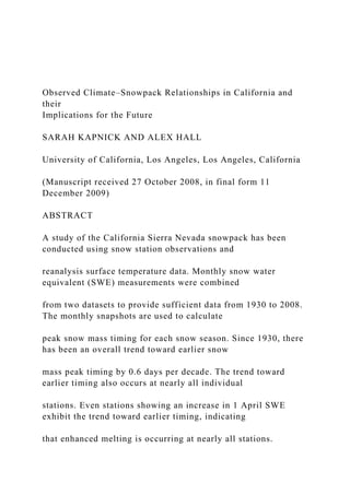
  • 21. March temperature 0.2 0.3 0.4 0.5 0.7 April temperature 0.0 0.1 0.1 0.3 0.5 May temperature 0.1 0.2 0.3 0.3 0.2 Averaged March and April temperature 0.1 0.2 0.3 0.4 0.6 FIG. 3. SCD for 22 stations with annual data available for at least 75% of the record from 1930 to 2008. There are 1482 data points for the time period. The dashed line denotes the mean SCD (Julian day 76) and the solid line denotes the linear trendline for the time series. 3450 J O U R N A L O F C L I M A T E VOLUME 23 c. Distribution of peak snow mass timing versus 1 April SWE Variability in 1 April SWE is evaluated against vari- ability in the SCD metric to explore relationships be- tween SCD and the SWE variable used to predict water supply. Figure 5 shows a scatterplot of 1 April SWE
  • 22. versus SCD values. Each point represents a snow station during one snow season. Snow stations with a minimum of 75% of SCD values over the period from 1950 to 2003 were used for this analysis. This time period was selected to coincide with the available temperature record and increase the number of snow stations available for tem- perature sensitivity studies in section 3d. (A nearly iden- tical distribution is found if the start date is changed to 1930.) For the given subset of snow stations, SCD occurs over a wide range, with the average SCD occurring on Julian day 73 (mid March). The average 1 April SWE value is 74 cm. The striking bell-shaped distribution of the 1 April SWE versus SCD scatterplot arises because of differing behavior of SCD for large and small seasonal snow accumulation. When 1 April SWE is large (roughly $100 cm), the SCD tends to occur in a narrow band between Julian day 70 and 90, with most points (96%)
  • 23. above the mean of 73. This corresponds to a time period mainly falling between the middle of the second and third bar of Fig. 2, or the calendar month of March. There are three main reasons for this behavior: 1) To attain such high 1 April SWE values, relatively consistent storm activity and steady accumulation is necessary from February to March. 2) The large accumulation then in- creases the effective thermal inertia of the snowpack, delaying the onset of melting. 3) This large accumulation then only melts once the seasonal warming becomes great enough to initiate the melting process. These three processes make for a late SCD, with little variation from season to season. When 1 April SWE is small (less than roughly 100 cm) however, the SCD falls over a large range between Julian day 21 and 114. This range is more than 4 times that of the high seasonal accumulation and covers the middle of the first bar to the middle of the fourth bar
  • 24. in Fig. 2, or from the last day in January to the end of April. The significantly greater range in SCD values is due to two factors: 1) Low accumulation is the re- sult of a relatively small number of storms with highly variable timing. 2) Melting in shallow snow is more sensitive to temperatures above freezing because of the smaller thermal inertia of shallow snow and its greater susceptibility to albedo feedback. This results in earlier (later) snowmelt when temperatures are warm (cold). To explore the sensitivity of SCD to temperature fur- ther, the colorbar given in Fig. 5 distinguishes the distri- bution of SCD values by local averaged March and April (MA) maximum daily temperature. The local average maximum daily temperature for each station is calcu- lated by taking the local gridcell maximum daily tem- perature, averaging it over two months, and adjusting it for the elevation of each station assuming a constant
  • 25. lapse rate of 6.58C km21. When the distribution of SCD versus 1 April SWE is distinguished by temperature, SCD has very little systematic association with either January or February temperatures, but is closely linked to early spring temperature (colorbar in Fig. 5). The correlations of observed SCD and temperatures for dif- ferent months are shown in the first row of Table 2, and clearly quantify the influence of late accumulation season temperature on SCD. Lower MA temperatures appear to shift SCD into the later half of the season. The most likely reason for this connection is that snowmelt dur- ing March and April is reduced (increased) by anoma- lously cold (warm) March and April temperatures, thus moving SCD to the later (earlier) portion of the season. The sensitivity to MA temperature is particularly pro- nounced for years when 1 April SWE is low (r 5 20.61, p , 0.01 when 1 April SWE is less than 100 cm versus r 5 20.47, p , 0.01 when it is above this threshold),
  • 26. providing direct evidence of the greater susceptibility of shallow snow to fluctuations in temperature and poten- tially albedo feedback. FIG. 4. Trend in SCD vs trend in 1 April SWE for 22 stations with at least 75% of years available from 1930 to 2008. Stations are the same ones used for Fig. 3. Dashed lines denote trends of zero. Stations are colored by elevation in meters. Circled stations have statistically significant trends (at p , 0.05) in 1 April SWE and SCD. Stations with a cross (x) have statistically significant trends (at p , 0.05) in 1 April SWE or SCD. 1 JULY 2010 K A P N I C K A N D H A L L 3451 d. Relationships between peak snow mass timing and temperature Figure 5 provides visual evidence that air temperature, the primary thermodynamic control of melt, is poten- tially a major variable affecting SCD. Figure 6a pro-
  • 27. vides a statistical measure of the link between the MA maximum daily temperature and SCD for the direct observations of these variables. Temperature is found to shift SCD earlier in the season by 2.5 days per degree and is significantly anticorrelated (r 5 20.62, p , 0.01) with SCD. As noted in section 3b, the trend toward ear- lier SCD coincides with a trend toward warmer MA temperature. The anticorrelation between SCD and tem- perature seen in Fig. 6a could result from these two trends. However, when the SCD and temperature time series are detrended, the anticorrelation remains (r 5 20.47, p , 0.01). This suggests the link between MA temper- atures and SCD is robust for temporal variability as well as trends in SCD, a point we return to in the discussion. Figures 6b,c reveal the SCD–temperature relationship when controlled for spatial and temporal variability. In Fig. 6b, the temporal SCD and maximum daily tem- perature anomalies (defined as the observation value
  • 28. minus the mean value at each station) are compared. Here we eliminate any systematic relationship between SCD and temperature in Fig. 6a arising from the fact that the stations are at different locations and therefore have different climatological temperatures. Conversely, in Fig. 6c, temporal variability is eliminated by com- paring station mean SCD values against station mean maximum daily temperatures. Thus, each point on the graph is an individual station. A negative relationship between SCD and temperature remains when spatial and temporal variability are each isolated in turn. More- over, Table 2 shows that MA temperatures have the greatest overall relationship with SCD from January to May for direct observations, anomalies, and mean sta- tion values. This analysis was also conducted using av- eraged daily minimum temperatures; negative correlations FIG. 5. Scatterplot of SCD vs 1 April SWE value for 70 stations with at least 75% of years
  • 29. available from 1950 to 2003; colored by the local averaged March and April daily maximum temperature. Temperature data are from the Hamlet and Lettenmaier (2005) dataset (avail- able from 1915 to 2003) and have been adjusted for station elevation assuming a constant lapse rate of 6.58C km 21 . If the graph is confined to stations with at least 75% of years available from 1930 to 2003, a similar distribution is found. The average SCD for the dataset is Julian day 73, and is given by the dashed black line. TABLE 2. Correlation of temperature vs SCD for 70 stations from 1950 to 2003 for January–May and for direct observations, anomalies, and mean values of these variables. This table provides a sensitivity analysis of the correlations found in Fig. 6 (the last column, bolded) for different months. Sensitivity January February March April May Averaged March and April Direct observation 20.21 20.21 20.56 20.52 20.28 20.62 Anomaly 0.04 0.02 20.52 20.49 20.10 20.65
  • 30. Station mean 20.55 20.60 20.65 20.60 20.60 20.63 3452 J O U R N A L O F C L I M A T E VOLUME 23 between SCD and temperature remained, but were lower than shown in Fig. 6 and Table 2. This is likely due to maximum temperature being more closely associated with snowmelt given that average minimum tempera- tures are predominantly below freezing. This analysis provides evidence of the predictive value of MA maxi- mum temperature for both spatial and temporal vari- ability in SCD. 4. Summary In this study, a metric is developed to calculate peak snow mass timing in the California Sierra Nevada using monthly SWE data from 1930 to 2008. Robust statisti- cal analysis is conducted to assess the variability in the timing of peak snow mass. From 1930 to present, the peak timing of the entire dataset exhibits a trend toward
  • 31. earlier in the season of 0.6 days decade21. On an in- dividual station basis, most stations show earlier SCD and reduced 1 April SWE, and the only stations with statistically significant trends in both SCD and 1 April SWE exhibit negative trends in both variables. The trends in SCD complicate interpretations of 1 April SWE as a metric of Sierra Nevada snowpack trends as nearly all stations exhibit negative trends in SCD indicating that enhanced melting is occurring even when 1 April SWE may be increasing. The influence of MA temperature on SCD is almost certainly due to the effect of early spring temperature on snowmelt. This relationship is particu- larly pronounced for low accumulation years, indicating the lower thermal inertia of shallow snow and potential enhancement of snowmelt due to albedo feedback as bare ground and vegetation is exposed. The robustness in the sensitivity of SCD to MA temperature for all spatial and temporal scales inherent in the dataset indicates
  • 32. the SCD trend can be attributed to the MA warming trend. The trend in snow mass peak timing found in this study is less than those of snowmelt-dominated streamflow found in some previous studies (Regonda et al. 2005; Stewart et al. 2005; Cayan et al. 2001), which provide changes in the date of peak runoff on the order of a few days per decade. The differences in the trends in these two metrics may be accounted for by the fact that a shift in the timing of streamflow runoff is not necessarily ac- companied by an equal shift in peak snow mass. In fact, FIG. 6. Scatterplot of averaged March and April daily maximum temperature vs SCD for 70 stations from 1950 to 2003 for: (a) ob- servations of SCD and local temperature, (b) anomalies, and (c) mean values. The dashed black line denotes the linear trendline on each graph. The two variables are strongly anticorrelated for all plots: (a) r 5 20.62, (b) r 5 20.65, and (c) r 5 20.63, with p , 0.01
  • 33. for all graphs. If the correlation is calculated for the detrended direct observations and detrended anomalies, the anticorrelations are slightly lower (r 5 20.47 in each case), but still material. 1 JULY 2010 K A P N I C K A N D H A L L 3453 if the shift in SCD is due to earlier snowmelt, the snow- melt acceleration would probably have to be much more rapid than the SCD shift. This is because of the steadi- ness of the weights of the accumulation months (i.e., measurements around 1 February and 1 March) in the SCD calculation. The involvement of four months of data in the SCD calculation introduces more ‘‘inertia’’ into this quantity than snowmelt runoff. 5. Discussion Taken together, this study and previous studies paint a picture of a California Sierra Nevada snowpack respond- ing rapidly to the changing climate of the past few de-
  • 34. cades. These trends are likely to continue and may be accelerating. Extrapolating the current trend in MA temperatures, peak snow mass timing should continue to occur earlier. Projections of temperature in California in the coming decades show that the trend in annual temperature may accelerate, with surface temperatures increasing by 28 to 78C by 2100 (Cayan et al. 2008). Assuming a similar distribution change in temperature in March and April, we can calculate a projection of the shift in SCD by the end of the century. Using the re- lationship between temperature and SCD anomalies in Fig. 6b, this implies a shift in the SCD from current mean values by 6 to 21 days earlier by the end of the century, with potentially much larger shifts in snowmelt runoff timing. These extrapolations into the future may be too con- servative because the trends in SCD found in this study are probably low estimates of future changes in peak
  • 35. snow mass timing. In addition to acceleration of climate change itself, snow season temperatures will begin to rise above the freezing point with increasing frequency as the climate continues to warm, leading to more pre- cipitation falling as rain instead of snow. On average, this threshold has not yet been reached for the given stations during the months of March and April. During March and April there were only two instances (less than 0.1%) of data points shown in Fig. 5 having average daily minimum temperatures above 08C. Most stations gener- ally exhibit net snow accumulation during this time pe- riod. As minimum temperatures begin to rise above the critical threshold of 08C much more often, melt rates will continue to increase, but precipitation will also shift from being dominated by snow to rain, which will eventually result in net melt rather than net accumulation in early spring. At present, January and February have both average daily maximum and minimum temperatures
  • 36. below freezing. If these winter months begin to expe- rience temperatures above freezing, less accumulation may occur during this time, making the snowpack more susceptible to temperature fluctuations later in the sea- son. Stations at lower elevations will be the first to ex- hibit changes in accumulation dynamics. This has been shown in Knowles et al. (2006), where sites at elevations below the majority of those in this study (below 1900 m) have exhibited a shift in cold season precipitation from snow to rain. The shift to rain will also impact SWE values in the latest part of the season first, which will contribute to the advance of SCD. The calculated sensi- tivity of SCD to late season temperatures does not reflect this mechanism yet, and therefore is probably a lower bound. Given the importance of high-resolution snowpack predictions, continued research on the California Sierra Nevada snowpack is critical to understanding the state’s
  • 37. future water supply. Continuation of SWE measure- ments is necessary to monitor and predict changes in the water supply from the Sierra Nevada snowpack. Re- gional modeling studies of the Sierra Nevada would also be helpful to determine the mechanisms affecting accu- mulation and melt events and to identify regions where precipitation will shift from being snow-dominated to rain-dominated. Snowmelt runoff will be affected by changes in snowfall amounts and snowmelt timing. An understanding of the mechanisms affecting these vari- ables will help predict the future of the California water supply. Acknowledgments. Sarah Kapnick is supported by an NASA Earth and Space Science Fellowship (#07-Earth07F- 0232) and a JPL fellowship (Earth Climate Science: Collaborative Investigations with UCLA Graduate Stu- dents: 1313181). Alex Hall is supported by UC Water Resources Grant WR1024. The writers would also like
  • 38. to gratefully acknowledge funding provided by JPL (#1312546) under a project entitled: ‘‘Evaluating key uncertainties in IPCC Climate Change projection of California snowpack: Topography, snow, physics and aerosol deposition.’’ APPENDIX Test of Snow Station Coherence If stations exhibit different accumulation patterns— entirely possible given their broad geographical and al- titudinal distribution—they must be treated as subgroups of data rather than as a single system to avoid over- generalization of the behavior of the snowpack. Under- standing the spatial variability of SWE is therefore a necessary step in our study. To achieve this, we calculate the spatial coherence of the monthly SWE values. The 3454 J O U R N A L O F C L I M A T E VOLUME 23 subset of stations for each month (taken within two weeks
  • 39. of the first of the month in February, March, April, and May) with yearly values available for 50% of the time period from 1930 to 2008 is used for this analysis. For each month, the time series of SWE values averaged over the state are calculated and then correlated with each individual station time series. The results are then plotted in Fig. A1. FIG. A1. Correlation plot to show spatial station coherence. Correlations are calculated on a first-of-the-month basis for (a) February, (b) March, (c) April, and (d) May. For the given month, correlations were calculated on a station-by-station basis between individual station SWE values against the mean SWE value for the set stations shown. Only stations with annual data for at least 50% of the record between 1930 and 2008 are used. There were 119, 120, 139, and 102 stations, respectively, in each month. 1 JULY 2010 K A P N I C K A N D H A L L 3455 We find that snow stations are generally highly spa- tially correlated with the mean SWE value for the snow-
  • 40. pack, especially those stations below 408N. For example, in the month of April, 110 stations have correlations to the mean SWE value above 0.80 with p , 0.01. This pattern persists from February to May, implying SWE anomalies are fairly uniform across the state for all months. These correlations may also be lower than if the analysis was conducted with actual first-of-the-month SWE values given that measurements are taken within two weeks of the first of the month. This measurement practice may introduce some error in these correlation calculations. However, the overall spatial coherence of snowpack variability demonstrates that minor tempo- ral gaps at individual stations will not materially affect analysis of the climatology and variability of the overall California snowpack when the dataset is taken as a co- herent group. This finding is especially important for the trend analysis found in section 3b and shown in Fig. 3 as some stations do not have data over the entire time
  • 41. period of interest (1930 to 2008). Sensitivity analysis of calculated trends is also provided when stations with different temporal records are used (Table 1). It should be noted that the station below 408N with the lowest correlation to the mean SWE time series is also the station with the lowest elevation. This location likely has different meteorological conditions, temperature pat- terns, and may experience snowmelt earlier and more frequently throughout the snow accumulation season than points at higher elevation. Because of its aberrant behavior, this station is left out of other analysis con- ducted in this study. REFERENCES Aguado, E., D. Cayan, L. Riddle, and M. Roos, 1992: Climatic fluctuations and the timing of west coast streamflow. J. Climate, 5, 1468–1483. Barnett, T., and Coauthors, 2008: Human-induced changes in the
  • 42. hydrology of the western United States. Science, 319, 1080– 1083, doi:10.1126/science.1152538. Cayan, D., 1996: Interannual climate variability and snowpack in the western United States. J. Climate, 9, 928–948. ——, S. Kammerdiener, M. Dettinger, J. Caprio, and D. Peterson, 2001: Changes in the onset of spring in the western United States. Bull. Amer. Meteor. Soc., 82, 339–415. ——, E. Maurer, M. Dettinger, M. Tyree, and K. Hayhoe, 2008: Climate change scenarios for the California region. Climatic Change, 87 (S1), 21–42. Hamlet, A., and D. Lettenmaier, 2005: Production of temporally consistent gridded precipitation and temperature fields for the continental United States. J. Hydrometeor., 6, 330–336. ——, P. Mote, M. Clark, and D. Lettenmaier, 2005: Effects of temperature and precipitation variability on snowpack trends in the western United States. J. Climate, 18, 4545–4560. Huntington, T., G. Hodgkins, B. Keim, and R. Dudley, 2004:
  • 43. Changes in the proportion of precipitation occurring as snow in New England (1949–2000). J. Climate, 17, 2626–2636. Knowles, N., M. Dettinger, and D. Cayan, 2006: Trends in snowfall versus rainfall in the western United States. J. Climate, 19, 4545–4559. Lundquist, J., D. Cayan, and M. Dettinger, 2004: Spring onset in the Sierra Nevada: When is snowmelt independent of eleva- tion? J. Hydrometeor., 5, 327–342. Mote, P., 2006: Climate-driven variability and trends in mountain snowpack in western North America. J. Climate, 19, 6209–6220. ——, A. Hamlet, M. Clark, and D. Lettenmaier, 2005: Declining mountain snowpack in western North America. Bull. Amer. Meteor. Soc., 86, 39–49. Pierce, D., and Coauthors, 2008: Attribution of declining western U.S. snowpack to human effects. J. Climate, 21, 6425–6444. Regonda, S., B. Rajagopalan, M. Clark, and J. Pitlick, 2005: Sea-
  • 44. sonal cycle shifts in hydroclimatology over the western United States. J. Climate, 18, 372–384. Serreze, M., M. Clark, R. Armstrong, D. McGinnis, and R. Pulwarty, 1999: Characteristics of the western United States snowpack from snowpack telemetry (SNOTEL) data. Water Resour. Res., 35, 2145–2160. Stewart, I., D. Cayan, and M. Dettinger, 2004: Changes in snow- melt runoff timing in western North America under a ‘business as usual’ climate change scenario. Climatic Change, 62, 217– 232. ——, ——, and ——, 2005: Changes toward earlier streamflow tim- ing across western North America. J. Climate, 18, 1136–1155. 3456 J O U R N A L O F C L I M A T E VOLUME 23 Copyright of Journal of Climate is the property of American Meteorological Society and its content may not be copied or emailed to multiple sites or posted to a listserv without the copyright holder's express written
  • 45. permission. However, users may print, download, or email articles for individual use.