1. Mitigating supply chain disruptions through the assessment
of trade-offs among risks, costs and investments in capabilities
S. Vahid Nooraie a,1
, Mahour Mellat Parast b,n
a
Department of Industrial and Systems Engineering, North Carolina A&T State University, 1601 E Market Street, Greensboro, NC 27411, United States
b
Technology Management North Carolina A&T State University, 1601 E Market Street, Greensboro, NC 27411, United States
a r t i c l e i n f o
Article history:
Received 26 October 2014
Accepted 20 October 2015
Available online 29 October 2015
Keywords:
Supply chain risk management
Disruptions
Supply risk
Demand risk
Heuristic
a b s t r a c t
One of the central questions in supply chain design is how to properly invest in supply chain capabilities
in order to be more responsive to supply chain disruptions. This new perspective in supply chain design
requires an understanding of the relationships among costs, supply chain risk drivers, and investments in
supply chain capabilities. In this paper, we develop a multi-objective stochastic model for supply chain
design under uncertainty and time-dependency. Sources of risk are modeled as a set of scenarios, and the
risk of the system is determined. The objective is to examine the trade-offs among investments in
improving supply chain capabilities and reducing supply chain risks, and to minimize cost of supply
chain disruptions. Due to the NP-hard nature of the problem, a heuristic algorithm based on a relaxation
method is designed to determine an optimal or near-optimal solution. To examine the efficiency of the
heuristic algorithm, a numerical example is provided. Our findings suggest that increasing supply chain
capabilities can be viewed as a mitigation strategy that enables a firm to reduce the total expected cost of
a supply chain subject to disruptions.
& 2015 Elsevier B.V. All rights reserved.
1. Introduction
The design of a supply chain that can be efficient while
responsive to disruptions is a significantly complex and challen-
ging task (Christopher and Peck, 2004; Ponomarov and Holcomb,
2009; Pettit et al., 2010). Supply chain managers are striving to
achieve the goal of fully integrated supply chains that are efficient
and competitive, yet responsive to risks and disruptions. This is a
daunting task due to the inherent risks in global supply chains,
ranging from demand uncertainty to environmental turbulence
(Chopra and Sodhi, 2004; Roh et al., 2014). While investment in
supply chain capabilities increases the ability of the firm to be
more resilient and responsive to supply chain disruptions, it has its
own costs (Juttner, 2005; Chopra and Sodhi, 2014). Thus, organi-
zations are faced with the evaluating the cost-benefit of invest-
ments in supply chain capabilities to address supply chain risks.
Although a focus on the design of efficient supply chains has
helped organizations reduce their costs, it has increased their vul-
nerability to disruptions (Wright, 2013). Previous studies show that
due to economies of scale, firms would be able to minimize their fixed
cost through minimizing investment in the number of facilities
(Goetschalckx et al., 2013; Huang and Goetschalckx, 2014). Thus,
addressing the overall effectiveness of a supply chain requires exam-
ining the trade-off between investments in supply chain capabilities
and the costs associated with disruptions. This requires a significantly
different approach to supply chain design, using a perspective that
incorporates the responsiveness and resiliency of a supply chain.
In recent years, academics and practitioners have focused on
supply chain risks and the impact of such risks on supply chain
design decisions (Blackhurst et al., 2005; Craighead et al., 2007;
Elkins et al., 2005; Hendricks and Singhal, 2003, 2005; Kleindorfer
and Saad, 2005; Rice and Caniato, 2003; Tang, 2006). A great deal of
work has focused on evaluating different sources of risk and dis-
ruption in supply chains, and how firms can develop mitigation
strategies to respond to disruptions. Nevertheless, there is a gap in
the literature on the trade-off between increased investment in
supply chain capabilities and reduced supply chain risks. Chopra
and Sodhi (2014) discuss the importance of development and
implementation of risk management plans that reduce risks with
limited impact on cost efficiency. While there is some anecdotal
evidence on the benefits of implementing risk management plans,
the cost-effectiveness of these programs has not been fully exam-
ined. To address this gap in the literature, we aim to provide a more
holistic assessment of the trade-off between investment in supply
chain capabilities and minimizing supply chain risk and cost.
The study makes two contributions to the literature in supply
chain risk management. It develops a decision model for supply
Contents lists available at ScienceDirect
journal homepage: www.elsevier.com/locate/ijpe
Int. J. Production Economics
http://dx.doi.org/10.1016/j.ijpe.2015.10.018
0925-5273/& 2015 Elsevier B.V. All rights reserved.
n
Corresponding author. Tel.: þ336 285 3111.
E-mail addresses: Snooraie@aggies.ncat.edu (S. Vahid Nooraie),
mahour@ncat.edu (M.M. Parast).
1
Tel.: þ336 285 3723.
Int. J. Production Economics 171 (2016) 8–21
2. chain risk management with respect to the tradeoff between the
cost associated with supply chain disruptions and the revenue
generated as the result of investment in supply chain capability,
where supply chain capability as investment in new facilities, pro-
ducts sites, and distribution channels, which are usually regarded as
improving redundancy in the supply chain design. The existing
studies in supply chain design do not examine the impact of supply
chain capability on mitigating supply chain disruptions. Previous
studies (e.g. Guille'n et al. (2005)) provides a decision model for
supply chain under uncertainty. However, whether firms would be
able to mitigate supply chain disruptions through investment in
supply chain capability remains unclear. Chopra and Sodhi (2014)
argued that managers usually do not invest in supply chain cap-
abilities because they view these investment as costs. We deter-
mine whether decisions to improve supply chain capability through
investment in supply chain components such as facility, plant, and
distribution channels has a positive impact on mitigating supply
chain disruptions and minimizing supply chain cost. Such an
approach to supply chain design has important managerial impli-
cations since manager would be able to incorporate supply chain
risk decision into their supply chain design as part of their supply
chain practices. Methodologically, we develop a heuristic algorithm
to find the (near) optimal solution due to the NP-hard nature of the
model. This algorithm is new and novel, which is used for problems
that have binary variables and optimum solution is not always
accessible for large scale problems, which is an extension of the
method proposed by Narenji et al. (2011).
The remainder of this paper is organized as follows. In the next
section, we discuss the importance of supply chain design as a risk
mitigation strategy, and examine the scholarly work on supply
chain risk management. Later, we introduce a multi-objective
supply chain model that incorporates supply chain capability
investment, supply chain risks and costs. Then we provide model
interpretations and define our heuristic method based on a
relaxation and decomposition method. Finally, we discuss the
findings of the study, its contribution to the theory and practice of
supply chain risk management and directions for future research.
2. Supply chain design as a risk mitigation strategy
While supply chain design may involve many strategic, tactical and
operational decisions, most supply chain design decisions are concerned
with location decisions, i.e., where to locate facilities such as plants,
processing units, warehouses, and retail stores to minimize the total
cost of transportation (Speier et al., 2011). With the emergence of
integrated logistics, integrated manufacturing, and strategic procure-
ment, supply chain design goals have expanded beyond their limited
focus on cost, and have begun to focus on minimizing the total landed
cost, including factors such as material acquisition, production, inven-
tory, and logistics (Bowersox et al., 2006). Further developments in
supply chain design have incorporated the idea of segmental customer
service requirements, which proposes that manufacturers need multi-
ple supply chains to satisfy the individual service requirements of dif-
ferent customer segments while also being efficient and cost-effective.
This approach attempts to minimize total delivered cost while devel-
oping innovative design strategies to satisfy delivery requirements in
terms of time and availability (Speier et al., 2011). We propose a new
perspective on supply chain design where we incorporate supply chain
capabilities into the design of the supply chain, and the objective of
satisfying customers is achieved through minimizing the risk and
increasing the responsiveness of the supply chain to disruptions.
2.1. Supply chain capability
Supply chain capability refers to the ability of an organization to
identify, use, and assimilate both internal and external resources
and information to facilitate supply chain activities (Bharadwaj,
2000; Wu et al., 2006). Previous research classifies supply chain
capabilities into efficiency-related and efficacy-related capabilities
(Chen et al., 2009). Efficiency-related capabilities enable firms to
reduce the cost of logistics and supply chain activities (Wu et al.,
2006; Chen et al., 2009), while efficacy-related capabilities allow
organizations to maintain keep connections with supply chain
participants as well as respond to consumer needs (Chen et al.,
2009; Kim et al., 2006). Morash and Lynch (2002) view supply chain
capabilities as logistics-oriented capabilities and customer-service-
oriented capabilities. In this research, we use both efficiency-related
capabilities and efficacy-related capabilities, because we minimize
transportation cost as well as responding to customer demands
(Rajaguru and Matanda, 2013).
3. Literature review
Supply chain risk management (SCRM) is defined as the
development and implementation of strategies to manage both
day-to-day and exceptional risks along a supply chain, with the
objective of reducing vulnerability and ensuring business con-
tinuity (Zsidisin et al., 2005; Wieland and Wallenburg, 2012).
Sources of risk include (but are not limited to) supply disruptions,
demand fluctuations, environmental uncertainty and turbulence,
equipment breakdown, procurement failures, and forecast inac-
curacies (Harland et al., 2003; Zsidisin, 2003; Chopra and Sodhi,
2004; Spekman and Davis, 2004).
In order to minimize the impact of disruptions on supply chain
performance, several attempts have been made to model and
optimize supply chain design, mostly utilizing a deterministic
approach to supply chain modeling and analysis (Timpe and
Kallrath, 2000; Gjerdrum et al., 2001; Azaron et al., 2008). How-
ever, most real supply chain design problems are characterized by
multiple sources of risks and uncertainties inherent in the design
of such systems. Thus, in order to obtain a more realistic assess-
ment of supply chain risks and their impact on supply chain per-
formance, the model parameters such as cost coefficients, supplies,
and demand should be implemented in a stochastic model.
Few research studies have used two-stage stochastic models to
examine the comprehensive design of supply chain networks. Mir-
Hassani et al. (2000) considered a two-stage model for multi-period
capacity planning of supply chain networks. The authors applied a
Benders decomposition to solve the resulting stochastic integer pro-
gram. Santoso et al. (2005) unified a sampling strategy with an
accelerated Benders decomposition to solve supply chain design pro-
blems assuming continuous distributions for the non-deterministic
parameters. They designed a computational model involving two real
supply chain networks to highlight the significance of the stochastic
model as well as the efficiency of the proposed solution strategy. Goh
et al. (2007) developed a probabilistic model of the multi-stage global
supply chain network problem, assuming supply, demand, exchange,
and disruption as the deterministic parameters. Azaron et al. (2008)
developed a multi-objective stochastic programming approach for
supply chain design under uncertainty.
It should be noted that assessment of the optimal supply chain
configuration is a real challenge, because many factors and
objectives must be assumed when designing the network under
uncertainty. However, the robustness of such a decision to non-
deterministic parameters is not considered in the above cases. To
overcome the above limitations, this paper considers the mini-
mization of the expected total cost, and the financial risk in a
S. Vahid Nooraie, M.M. Parast / Int. J. Production Economics 171 (2016) 8–21 9
3. multi-objective model to design a robust supply chain network.
Such an approach in using expected value to reduce model com-
plexity is suggested in previous studies (e.g., Li et al. (2013), Aiello
et al. (2015), Nooraie and Parast (2015)). We follow the recent
developments in multi-objective optimization through utilizing
the concept of solution robustness; we assume stability of an
optimal solution, considering errors in the objective function
parameters (Cromvik et al., 2011).
3.1. Methodological approaches
Huang and Goetschalckx (2014) and Goetschalckx et al. (2013)
proposed supply chain systems when there are a large number of
discrete configurations. Sources of risks are modeled as a series of
scenarios. The risk of the supply chain is formulated as the stan-
dard deviation of the revenues of the different scenarios. An
optimizing algorithm that efficiently determines all Pareto-
optimal figures of a supply chain is determined. The results
show that a general risk mitigation strategy for supply chains is to
enhance the total capacity of the supply chain by either building
more facilities or by raising the capacity of individual facilities.
Many methods and approaches have been applied to solve problems
connected to supply chain design. These methods include mathematical
modeling, heuristics and artificial intelligence. In recent years, alter-
native methods have been applied; one of the most widely used is
meta-heuristics. Although such methods are not guaranteed to provide
an optimal solution, they make a helpful compromise between the
measure of computation time spent and the quality of the approxi-
mated solution area. Silva et al. (2005) offered a supply chain design as a
logistic process that comprises order arrival, components request,
components arrival, components assignment and order delivery. The
case is to define the sequence in which orders should be performed.
The ensuring scheduling problem is solved applying Genetic Algorithms
(GA) and Ant Colony Optimization (ACO). Altiparmak et al. (2006)
offered a method, based on GA, for designing a four-echelon supply
chain (suppliers, plants, warehouses and customers).
Several heuristic techniques such as Simulated Annealing (SA) and
GA have been used on a number of problems. First, ACO was used on
decision problems including a single objective. Later efforts inserted a
second objective or multiple objectives (McMullen, 2001; Doerner et al.,
2004, 2006, 2008; Stummer and Sun, 2005). McMullen (2001) devel-
oped a multi-objective production sequencing case where the objec-
tives are the number of set-ups and the stability of materials used. A
single combined pheromone matrix is applied in this technique.
Moncayo-Martіnez and Zhang (2011) proposed an algorithm based on
Pareto Ant Colony Optimization as an effective meta-heuristic technique
for solving multi-objective supply chain design problems. This techni-
que is efficient but rather complex; when the dimension of the problem
increases, the complexity increases dramatically.
Guille´n et al. (2005) developed a supply chain model using a
multi-objective stochastic Mixed-Integer Programming (MIP)
approach in which uncertainty is examined with demand forecasting.
The model is solved by branch and bound techniques. Objectives are to
maximize profit over the time period, maximize demand satisfaction
and minimize financial risk. While mathematical models have the
advantage of providing the optimal solution, the level of complexity of
an NP-hard problem requires too much computation for mathematical
calculation to be a realistic approach. Thus, the development of
alternative methodological approaches is needed (Dabia et al., 2013).
In this paper, we develop an efficient heuristic method where
branch and bound methods cannot be used to determine the
optimal solution. Our heuristic method does not guarantee an
optimal solution, but it provides a near-optimal solution where the
deviation between near-optimal and optimal is negligible.
3.2. Sources of risk in the supply chain
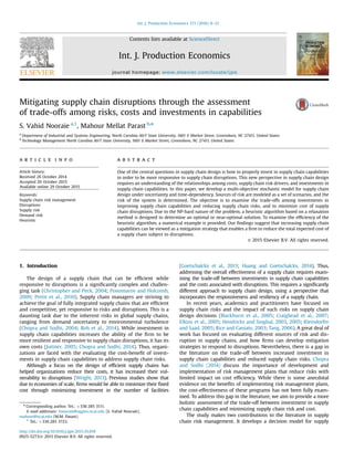
The scope of our model includes supply, process, demand and
control under risk. Fig. 1 presents the conceptual model of our supply
chain risk scope, where all main elements of supply chain design are
under risk (Christopher and Peck, 2004). In our model, we define risk as
probabilistic scenarios that have a direct effect on the value of our
model parameters.
The availability of more facilities provides more capability to
overcome disruptions and risks; however cost of facility establish-
ment and deployment should be considered (Chopra and Sodhi,
2004; Talluri et al., 2013; Chopra and Sodhi, 2014). This perspective
provides a more balanced approach toward supply chain risk man-
agement in which the benefits of establishing more facilities (cap-
abilities) should be examined in view of the associated risks and
costs within the supply chain. In other words, the design of supply
chain systems should examine the associated costs of trade-offs
among capabilities, risks and vulnerabilities (Pettit et al., 2010, 2013).
In this research, we examine the effectiveness of a supply chain
design system through investment in new facilities such as
warehouses, distribution centers and manufacturers to meet cus-
tomer needs in the face of disruptions. All of our parameters are
assumed time-dependent, because the time factor has a con-
siderable effect on the value of the model parameters. We will
develop an efficient heuristic method to identify all feasible
solutions based on a decomposition method to break MIP into sub-
linear models, and to compute the relaxed binary variables. To
evaluate probabilistic scenarios, we calculate the expected value
for each parameter. This heuristic method is based on the devel-
opment of previous heuristic methods for situations when the
model is NP-hard and complex (Narenji et al., 2011).
4. Problem description
In the strategic design of supply chains, there are possibly
several parameters whose measures cannot be determined accu-
rately, and their values are considered to be stochastic. In our
model, the probability of each scenario is determined as a discrete
value and we use the expected value approach to evaluate it.
Moreover, each scenario is time-dependent and dynamically
affects all parameters. In other words, the probability of each
scenario is not fixed, and it is changed during the time horizon
(Huang and Goetschalckx, 2014).
The main idea is to develop a model to maximize total revenue
and minimize total cost related to opening new facilities: ware-
houses, distribution centers and manufacturers. Our objective is to
find an optimal point as a trade-off between revenue and cost, to
understand how the establishment of new facilities (i.e. capabilities)
affects disruptions and risk while meeting customer demands.
Overall, we need to design a supply chain that incorporates risk of
disruptions, and to determine whether more investment in cap-
abilities and facilities enhances supply chain responsiveness to
disruptions. Thus, the goal is to understand how much investment
in new facilities is justified to mitigate supply chain risks, and to
determine the trade-off between costs and investment in cap-
abilities in a supply chain that is exposed to risks.
Process
Risk
Environmental Risk
Demand
Risk
Supply
Risk
Control
Risk
Fig. 1. Scope of supply chain risk management.
S. Vahid Nooraie, M.M. Parast / Int. J. Production Economics 171 (2016) 8–2110
4. In the next section, we define the mathematical formulations
for the multi-objective supply chain problem. Then, we define the
notation and decision variables, and present the mathematical
model for a multi-objective stochastic supply chain.
4.1. Notation and model variables
Sets and Indices
S: set of supplier facilities
C: set of customer facilities
W: set of warehouse facilities
DC: set of distribution centers
F: set of manufacturing factories
T: set of transformation facilities: T ¼ F [ DC [ W (union of F,
DC, and W is the definition of transformation facilities)
N: set of all facilities: N ¼ S [ C [ T (N is the union of all
facilities)
A: set of channels: A¼{(i, j) | i, jA N} (channels come from any
combination of F, DC, W, S, C and T)
SC: set of scenarios
K: set of products
TP: set of time periods (total of different time periods forms the
set of time periods, for instance, seasonal periods and yearly
periods)
Parameters
copenk
sit: the cost for establishing facility i to produce product k,
i.e., its initial investment cost
under scenario s in period t
Popenk
sit: the revenue from facility i from product k, under sce-
nario s in period t
ps: the probability of scenario s,
P
s
ps ¼ 1
ctransk
sijt: the unit cost to transport product k from location i to
location j under scenario s in period t
capk
slt: the capacity for product k of facility l under scenario s in
period t
dem
k
slt: the forecast demand for the product k of customer l
under scenario s in period t
supk
slt: the supplier capacity for product k of supplier l under
scenario s in period t
srk
sct: the unit sales revenue for product k sold to customer c
under scenario s in period t
Variables
yi: binary variable equal to 1 if facility i is opened and equal to
0 otherwise
xk
sijt: the flow variable for the product k from location i to loca-
tion j under scenario s in period t
exp z1: the expected value of objective function z1, the first
objective function is the maximization of total revenue, where
ps is the probability of each parameter
exp z2: the expected value of objective function z2, the second
objective function is the minimization of total cost, where ps is
the probability of each parameter
Expected value of Z1 ¼
P
s
ðps  z1Þ
Expected value of Z2 ¼
P
s
ðps  z2Þ
Note that the model can be expanded to handle multiple per-
iods that correspond to seasons in the planning horizon.
4.2. Mathematical model for multi-objective stochastic supply chain
disruption
Following the procedure suggested by Nooraie and Parast (2015),
the trade-off between investment in supply chain capability and
costs is formulated as the expected values of Z1 and Z2.
Max Z1 :
X
s
ps
X
c A C
X
k
X
t
srk
sct
X
i;cð Þ AA
X
t
xk
sict
1
A
0
@
þ
X
s
ps
X
iA T
X
t
Popensit
1
A Â yi 8Y; 8sϵSC
0
@ ð1Þ
Min Z2 :
X
s
ps
X
i;jð Þ A A
X
t
ctransk
sijt  xk
sijt
1
A
0
@
þ
X
s
ps
X
i AT
X
t
Copensit
1
A Â yi 8Y; 8sϵSC
0
@ ð2Þ
s.t.
X
i;lð ÞϵA
X
t
xk
silt À
X
l;jð ÞϵA
X
t
xk
sljt ¼ 0 8kAK; 8lϵT; 8sASC; 8tATP ð3Þ
X
i;lð ÞϵA
X
t
xk
silt rcapk
slt  yl 8kAK; 8lϵT; 8sASC; 8tATP ð4Þ
X
l;ið ÞϵA
X
t
xk
slit rsupk
slt 8kAK; 8lϵS; 8sASC; 8tATP ð5Þ
P
i;lð ÞϵA
P
t
xk
silt rdemk
slt 8kAK; 8lϵC; 8sASC; 8tATPyiϵ 0; 1f g 8iAT
ð6Þ
The objective function (1) is the expected value of the total
revenue of opening facilities and revenue of selling products as
well. The objective function (2) is the expected value of the total
cost of opening facilities and transportation cost of products as
well. Constraint (3) is a flow constraint that ensures that the input
quantity for each product is equal to the output quantity in each
facility; it means that the arrival products to each manufacturer
(F), warehouse (W), and distributer (DC) are equal to the products
that leave these facilities. Constraint (4) ensures that material
quantities do not exceed the given capacity. Constraint (5) enforces
that a supplier does not provide more of a product than its capa-
city for that product. Constraint (6) ensures that the quantity of
the finished products delivered to the customer does not exceed
the demand for the customer.
4.3. Model descriptions
Our model consists of the main elements of a supply chain
system: suppliers, manufacturers, warehouses, distribution cen-
ters and customers (Fig. 2). We can choose several numbers for
each element, as each element has a one-to-many relation with
the next elements in the supply chain; therefore, we have different
channels within the supply chain. The summation of the manu-
facturers, warehouses, and distribution centers is equal to T.
Moreover, T and the summation of suppliers and customers is
Supplier (S) Manufacturer (F) Warehouse (W) Distributer (DC) Customers (C)
S F W DC C
Supply chain channels
CDUWUF=T
N = S U C U T
Fig. 2. Graphical model of the facilities in a supply chain design.
S. Vahid Nooraie, M.M. Parast / Int. J. Production Economics 171 (2016) 8–21 11
5. equal to N, suggesting that the summation of all elements in our
supply chain equals N. These definitions are useful when we need
to formulate and develop our mathematical model.
Constraint (3) includes all elements where k is a product, s is a
scenario, and t is a time period. In this constraint, suppliers and
customers are connected together via T, which is the summation
of manufacturers, distribution centers and warehouses; i comes
from a supplier and passing through F, W, and DC reaches the
customer. Based on different values of these parameters, we have
different channels. The arrival products to a manufacturer (F),
warehouse (W), or distributer (DC) are equal to the products that
leave these facilities. Fig. 3 shows balanced flows in the supply
chain (from supplier to the manufacturer, to the warehouse, to the
distribution center, and to the customer). Arrows show that each
element has a relationship with all next-stage facilities. Each
supplier has a relationship with all manufacturers. The small
arrows on the upper side show that the quantity of materials
moving between facilities is unchanged.P
i;lð ÞϵA
P
t
xk
silt À
P
l;jð ÞϵA
P
t
xk
sljt ¼ 0 8kAK; 8lϵT; 8sASC; 8tATP
Constraint (4) includes all elements except the customer, where
k is a product, s is a scenario, and t is a time period. Fig. 4 shows
that there is a capacity limit in each element of T that affects each
previous facility, where T is a combination of the manufacturer, the
warehouse and the distribution center. Based on the capacity limit
for each combination of T elements, there is a limit for product k
from location i under scenario s in period t. This constraint ensures
that material quantities do not exceed the given capacity. There
are M Â N relations between elements; upper arrows from right to
left show that the capacity of each element affects previous ele-
ments in the chain. For example, the capacity limit of a manu-
facturer affects supplier output.
X
i;lð ÞϵA
X
t
xk
silt rcapk
slt  yl 8kAK; 8lϵT; 8sASC; 8tATP
Constraint (5) includes all elements where k is a product, s is a
scenario, and t is a time period. Fig. 5 shows that product k from
location i under scenario s in period t should be produced, con-
sidering the supplier limit provided by supplier l to produce pro-
duct k under scenario s in period t. This constraint enforces that a
supplier does not provide more of a product than its capacity for
that product. The upper arrow shows that the capacity limit of a
supplier affects the next element in the chain, which is a manu-
facturer.
X
l;ið ÞϵA
X
t
xk
slit rsupk
slt 8kAK; 8lϵS; 8sASC; 8tATP ð7Þ
Constraint (6) includes all elements where k is a product, s is a
scenario, and t is a time period; i comes from a supplier with
different channels and is connected to the customer. Fig. 6 shows
that the quantity of the finished products delivered to the custo-
mer does not exceed the demand for the customer. The upper
arrow shows that customer demand affects warehouses.
X
i;lð ÞϵA
X
t
xk
silt rdemk
slt 8kAK; 8lϵC; 8sASC; 8tATP
4.4. Numerical example
A numerical example shows how the model determines the
optimal solution. After obtaining the solution, we use our pro-
posed heuristic algorithm to determine how the algorithm deter-
mines the solution, and how much deviation exists between the
optimal value and the heuristic solution. This numerical example
1
.
.
.
.
n
Sup F W DC J
n n n n n
= = =
Equal materials flow
Fig. 3. Constraint (3).
1
.
.
.
.
n
Sup F W DC
n n n n
Capacity limit from manufacturer, warehouse, distributer
Fig. 4. Constraint (4).
1
.
.
.
.
n
Sup
n
Supplier capacity limit
Fig. 5. Constraint (5).
Customer demand
DC
n
Fig. 6. Constraint (6).
S. Vahid Nooraie, M.M. Parast / Int. J. Production Economics 171 (2016) 8–2112
7. consists of two products, two periods, two scenarios, two suppli-
ers, two customers, two warehouses, two distribution centers, and
two manufacturers (the data is provided in Appendix A). To
eliminate the probabilistic aspects of scenarios, we calculate the
expected value for each parameter. To further reduce the com-
plexity of the model, we define only one objective function based
on minimization of cost minus maximization of revenue. Table 1
shows the cost of each component of facilities under each scenario
in each period. Facilities include suppliers, customers, warehouses,
distribution centers and manufacturers. Table 1 is the solution of
the model on decision variable xk
sijt, the flow variable of each
product under each scenario in each period, that moves between
facilities i and j, where i j come from all facilities.
According to the solution for this numerical example by Cplex
software, we see that all binary variables y1, y2, y3, y4, y5 and y6
take on the value of 1. This suggests that the optimal policy is
achieved when all manufacturers, warehouses, and distribution
centers are open. In this case, the objective function Z¼ À
$18,955,628. The negative symbol shows that the total cost is less
than total revenue. Gross revenue is the absolute value of this
negative amount (Gross revenue¼$18,955,628).
Dabia et al. (2013) showed that a multi-objective time-depen-
dent optimization problem is an NP- hard problem. The supply
chain risk management system presented in this study is a multi-
objective, time-dependent, and multi-item capacitated model.
Thus, it has a much higher level of complexity due to the number
of model parameters. To find the solution for such a complex
problem, we develop a heuristic algorithm to determine the near-
optimum or optimum value with minimum deviation from the
optimal solution (Figs. 7 and 8).
5. The heuristic algorithm
We examined the number of constraints, and we learned that
the redundancy of each parameter significantly affects total con-
straints. For instance, if the number of each parameter is equal to 2
(parameters include number of products, scenarios, periods, sup-
pliers, manufacturers, warehouses, distribution centers and
customers), we should define more than 500 constraints. Narenji
et al. (2011) reported that when the number of parameters
increases in MIP, a branch and bound algorithm is not capable of
providing the optimal solution. They proposed a heuristic algo-
rithm based on relaxation and decomposition methods. In this
paper, we use a relaxation method for binary variables to develop
our heuristic method. Based on maximization or minimization, we
need to define two types of heuristic methods for our objective
functions. Simply, our heuristic algorithm activates binary vari-
ables (yi ¼1) each time, and gives us a primary idea to perform
ideal combinations for the binary variables. We choose the best
combination of activated variables; then, we solve different LP
problems. We look for the best LP problems based on a greater
number of satisfied constraints.
5.1. Satisfied constraints method for minimization
This method determines the (near) optimal solution based on
satisfying the greatest number of constraints. This approach is
used when the goal is to minimize the objective function (Nooraie
and Parast, 2015). We need to follow all the following steps to
determine an optimal or near-optimal solution.
Step 1. Calculate Z when all binary variables are one (Yi¼1
where i ε T ), then set the upper bound Zupper to Z.
Step 2. For i¼1….T (for T¼F U DC U W, combination of manu-
facturers, distribution centers and warehouses), set Yi ¼1, set all
other Y¼0, and calculate Zi. Then for Z¼Zi………ZT allocate a
group number from 1….T
Step 3. Sort groups from minimum to maximum. We define j as
a combinations number of Yi where j¼2…T. For example: if j¼3,
it means that we should set Yi ¼1 for the first three sorted
groups, then calculate Z.
Step 4. Follow this algorithm:
Step 5. Compare all Z values from Steps 3 and 4 and report an
optimal or near-optimal solution based on the largest number of
satisfied constraints.
Table 1 (continued )
9 4 o9 44 67,500 0 0 0 2750 85,250 0 0
9 5 o9 54 0 0 0 0 0 0 0 0
9 6 o9 64 0 0 0 0 0 0 0 0
9 7 o9 74 0 0 0 0 0 0 0 0
9 8 o9 84 0 0 3577.5 0 88,000 0 0 93,500
9 10 o9 104 5850 0 0 71,100 2750 88,000 0 0
10 1 o10 14 0 0 0 0 0 0 0 0
10 2 o10 24 0 0 0 0 0 0 0 0
10 3 o10 34 0 0 0 0 0 0 0 0
10 4 o10 44 0 1800 0 0 0 0 0 0
10 5 o10 54 0 0 0 0 0 0 0 0
10 6 o10 64 0 0 0 0 0 0 0 0
10 7 o10 74 0 0 0 0 0 0 0 0
10 8 o10 84 0 0 0 67,500 0 0 99,000 0
10 9 o10 94 0 58,500 74,250 0 0 0 0 0
For j = 2…T define Yi’s=1 then calculate Z
and count the number of satisfied constraints
Zj < = upper
bound?
Yes No
j = j +1
Stop when j = T + 1
Fig. 7. Minimization algorithm.
For j = 2…T define Yi’s=1 then calculate Z
and count the number of satisfied constraints
Zj < = upper
bound?
Yes No
j = j +1
Stop when j = T + 1
Fig. 8. Maximization algorithm.
S. Vahid Nooraie, M.M. Parast / Int. J. Production Economics 171 (2016) 8–2114
8. 5.2. Satisfied constraints method for maximization
This approach is used when the objective function is defined
based on maximization. We need to follow the following steps for
optimal or near-optimal solution.
Step 1. Calculate Zupper when all binary variables are one (Yi¼1
where i ε T ), then set upper bound based on Zupper (Upper
bound¼Zupper).
Step 2. For i¼1….T (T is the combination of warehouse, manu-
facturer and distribution center) Yi¼1 while other Yis ¼0 and
calculate Z then for Z¼Z i………ZT allocate group number from
1….T
Step 3. Sort groups from Max to Min
We define j as a combinations number of Yi where j¼2…T
Step 4. Follow this algorithm:
Step 5. Compare all Z values from Steps 3 and 4 and report
optimum/near optimum based most satisfied constraints (See
Appendix B).
Now, we consider a situation when we are dealing with a large-
scale problem. In this situation, we are not able to determine the
optimal point due to the complexity of the model. According to the
heuristic algorithm, we have the following data for our numerical case.
According to Table 2, the most constraints satisfied belong to the
last row, where y1, y2, y3, y4, y5, and y6 are set to 1, and the optimal
solution is $18,955,628. In this case, we have no deviation between the
optimal solution and the solution from the heuristic algorithm.
To assess the efficiency of the heuristic algorithm, we generated
data on each parameter, and ran our heuristic for 70 times; we
compared the heuristic solutions with the optimum values. Our
findings suggests that the mean value of deviation between opti-
mum and heuristic solutions is less than 5%. Thus, we conclude
that our heuristic algorithm is robust enough.
6. Discussion
In this study, to solve an NP-hard problem related to supply
chain design under risks and disruptions, we designed a heuristic
algorithm based on a relaxation method and the number of satisfied
constraints. In the process of decision-making to choose the best
solution, different strategies affect our alternative solutions (Fig. 9).
The decision model can assist a manager to manage the trade-off
among investment, risk, and costs within a supply chain. Among
single Yi's (decision variables), the best choice is Y1, where the
objective function is $16,464,764 and deviation from the optimal
solution is 13%. In the case of using a balanced emphasis on each
objective function (50% weight is given to each objective function),
the closest choice (where cost and revenue have almost equal
weights) is the combination of Y6, Y5, Y4 and Y3, where the
objective function is equal to $17,406,096 and the deviation is 10%.
In our model, we are interested in opening facilities as much as
possible, because more active facilities provide us more revenue
and the capability to cope with more cost and risk within the
supply chain. This is well in line with the notion of enhancing
redundancy in supply chain systems in order to mitigate the
negative impact of disruptions (Christopher and Peck, 2004; Sheffi,
2005; Sheffi and Rice, 2005; Zsidisin and Wagner, 2010). There-
fore, our alternative solution is based on y6, y5, y4, y3 and y2
binary variables, and the objective function is $17,406,096, where
deviation from the optimal solution is only 5%.
Our results show that we would be able to use the heuristic
method to estimate the optimal solution when we have a large-
scale NP-hard problem. We should mention that due to the NP-hard
nature of the problem, the optimal solution would not be deter-
mined easily. The relaxation method is very efficient, since devia-
tion of the heuristic solution from the optimal solution is negligible.
Based on this strategy, for example, if our objective function is
minimization, we need to sort binary variables from minimum to
maximum; then, we need to set the objective function based on
various combinations of binary variables. This method (sorting
binary variables) provides near-optimal or optimal solutions.
According to our findings, if we activate all facilities and expand
capabilities, the result of the objective function shows a trade-off
between total revenue and total cost. Opening all facilities provides
more capability to meet customer demands (efficacy-related cap-
ability) as well as minimizing transportation costs (efficiency related
capability). According to the probabilistic nature of scenarios, each
scenario directly affects all parameters because we use the expected
value technique, which decreases the real value of each parameter.
Furthermore, such probabilistic risks deviate from both total revenue
and total cost. This suggests that the results always are an approx-
imation of real amounts, and deviations are determined based on
risk probabilities. If the probability of a scenario is high, our heuristic
algorithm solutions have less deviation from the actual value.
Table 2
Satisfied constraints heuristic approach for minimization.
Yi Cost Revenue Profit¼Cost-Revenue Profit¼|Cost-Revenue| Upper-bound
Min 6 $2,052,416 $17,723,155 À$15,670,739 $15,670,739 $18,955,628
5 $2,113,465 $17,803,695 À$15,690,230 $15,690,230 $18,955,628
4 $2,027,103 $17,841,795 À$15,814,692 $15,814,692 $18,955,628
3 $2,402,493 $18,266,139 À$15,863,646 $15,863,646 $18,955,628
2 $1,872,173 $17,747,859 À$15,875,686 $15,875,686 $18,955,628
Max 1 $2,022,575 $18,487,339 À$16,464,764 $16,464,764 $18,955,628
65 $2,812,988 $18,940,071 À$16,127,083 $16,127,083 $18,955,628
654 $3,487,199 $20,195,087 À$16,707,888 $16,707,888 $18,955,628
6543 $4,468,351 $21,874,447 À$17,406,096 $17,406,096 $18,955,628
65432 $5,033,388 $23,035,527 À$18,002,139 $18,002,139 $18,955,628
654321 $5,980,459 $24,936,087 À$18,955,628 $18,955,628 $18,955,628
$0
$20,00,000
$40,00,000
$60,00,000
$80,00,000
$1,00,00,000
$1,20,00,000
$1,40,00,000
$1,60,00,000
$1,80,00,000
$2,00,00,000
|Cost-Profit|
Lowerbound
Middle bound
Upperbound
Fig. 9. Minimization algorithm (numerical example).
S. Vahid Nooraie, M.M. Parast / Int. J. Production Economics 171 (2016) 8–21 15
9. 6.1. Theoretical contributions
In this study, we developed a supply chain risk management model
where the tradeoffs among risks, supply chain costs and investment in
supply chain capabilities were examined. We added a time parameter
to the basic model to investigate the effect of time-dependency on all
parameters, where risks of disruption were incorporated into the
supply chain design. We also realize that a time parameter imposes
more complexity on the model. Moreover, we used expected value to
eliminate the stochastic nature of scenarios. We investigated the
trade-off between risk, cost and revenue, where more facilities provide
more capability to meet customer needs, and decrease the negative
effect of disruptions. Our finding shows that among those invest-
ments, any combination of facilities (manufacturer, distribution center
and warehouse) that can satisfy customer demand decreases the risk
of lost sales and lost revenue. It is important that we have to be
concerned with the total cost. It is very clear that we need to increase
the total revenue through increasing total capabilities, while the total
cost should be decreased as much as possible.
We designed a heuristic method to reduce the complexity of the
model due to the NP-hard nature of a multi-objective time-
dependent optimization problem (Dabia et al., 2013). Our model can
be applied when we need to meet customer needs in a risky
environment where the capability of each facility decreases the
impact of risks that are defined as probabilistic scenarios. In addi-
tion, our heuristic method is efficient, and can be applied where
there are several objective functions with opposite directions.
6.2. Managerial implications
Our model includes two main goals. The first one is based on
investment in new facilities that provide financial benefits through
increasing revenue; the second goal is to minimize the total cost of
the supply chain under risks. Our mathematical model is a type of
decision-making tool that a manager may use to examine decisions
regarding investment in developing new capabilities in a supply
chain vis-à-vis the cost associated with development of these cap-
abilities to mitigate disruptions and risks in the supply chain.
By evaluating the sources of risk and their frequency, a manager
would be able to evaluate how to design the proper supply chain to
mitigate the effects of those risks. For example, assume a manger has
intended to invest in a food supply chain in Florida, where tsunami,
storm and other natural disasters pose significant risks to the supply
chain. If the probability of tsunami in Florida is estimated to be
around 80–90%, that high level of risk could have a significant impact
on customer demand. In this situation, the supply chain manager
should estimate the future demands with a lower probability (e.g.,
45–55%); thus, we expect a much higher deviation of the expected
value for demand from the actual demand, due to the higher level of
environmental risk, as presented in the numerical example. Alter-
natively, when the risk of tsunami or other natural disasters are on
the lower side (e.g. 10–20%), the future demand would be more
stable, and the supply chain manager would be able to predict future
demand with more certainty, as the expected value for demand is
much closer to the actual demand. The parameters in our model
assist managers to evaluate the cost of facilities, revenue of facilities,
transportation cost, production capacity, customer demands, supplier
capacity and product revenue. The numerical results of the mathe-
matical model give a clear vision to the manager to decide on
opening manufacturers, warehouses and distribution centers in order
to be more responsive to supply chain disruptions.
6.3. Limitations and future research
In this research, the risk was measured as the expected value of
parameters. Various other risk measures have been proposed in
the literature and in stochastic optimization (Goetschalckx et al.,
2013). Examples are downside risk, conditional value at risk and
upper partial mean of the scenario profits. Investigation of those
risk measures, their relationships, and their impact on the supply
chain configuration is a fertile area of future research. Different
risk measures may also require the development of different
optimization and heuristic algorithms.
Another interesting area of research is the impact of other
capabilities such as agility and responsiveness in our model. In
addition, to prevent generating lower probabilities for risks, future
research should consider efficient solution techniques for high risk
scenarios. Alternatively, we can assume that our model is com-
pletely deterministic and there is no probabilistic risk in our
problem. In this case, we will have an accurate solution when we
already have designed preventive policies to mitigate risk situa-
tions or improve our supply chain design through investment in
other capabilities using new techniques such as flexibility.
7. Conclusion
The strategic design of a supply chain system is very important to
the long-term profitability and survival of firms. One of the key ques-
tions in supply chain design is how to determine the trade-off between
the capability of the supply chain (investment) and vulnerability to
supply chain disruptions under a variety of uncertain future conditions
(its risk). Firms would be able to decrease the negative impact of risks
through investment in more capabilities; however these investments
increase costs as well. Therefore, in supply chain design, we need to
examine investment in capabilities and their associated costs.
While obtaining an optimal solution for the model is a chal-
lenge due to the NP-hard nature of the problem, one efficient way
to make an informed decision on the trade-off involved in
designing a supply chain from a risk management perspective is to
use the largest number of satisfied constraints heuristic approach
and the corresponding solution algorithms.
Acknowledgment
This research is based upon work supported by the National
Science Foundation (NSF) under Grant number 123887 (Research
Initiation Award: Understanding Risks and Disruptions in Supply
Chains and their Effect on Firm and Supply Chain Performance).
Appendix A. Solution Results
Table A2 shows the expected values of the entries in Table A1.
(We use the expected value method to make deterministic values.)
Opening each facility in each period under each scenario for
each product generates revenue that is shown in Table A3. The
expected values of these numeric entries are shown in Table A4.
Table A5 shows transportation between facilities (supplier,
manufacturer, warehouse, distributer and customer facilities) for
each product, scenario, and time period separately (These data are
based on the expected values).
Table A6 shows that our model is capacitated, because each
facility (manufacturer, warehouse and distributor) has a capacity
constraint based on different periods, scenarios and products.
Table A7 shows the expected values for these entries.
Table A8 shows the customer demand that comes from demand
forecasting, where it varies by scenario, product, time period, and
customer. Table A9 shows the expected values of customer demand.
S. Vahid Nooraie, M.M. Parast / Int. J. Production Economics 171 (2016) 8–2116
10. Table A1
Cost of establishing facility i under scenario s in period t.
Copensit Scenario s 45% 55% 45% 55%
facility Period t 1 2
I S1 $ 100,000 $ 125,000 $ 300,000 $ 450,000
I S2 $ 150,000 $ 148,000 $ 250,000 $ 300,000
I C1 $ 250,000 $ 143,000 $ 115,000 $ 155,000
I C2 $ 300,000 $ 147,000 $ 450,000 $ 477,500
I W1 $ 450,000 $ 160,000 $ 376,000 $ 461,000
I W2 $ 500,000 $ 117,000 $ 394,000 $ 484,000
I DC1 $ 550,000 $ 112,000 $ 410,000 $ 502,500
I DC2 $ 600,000 $ 82,000 $ 430,000 $ 525,000
I F1 $ 700,000 $ 390,000 $ 465,000 $ 565,000
I F2 $ 750,000 $ 555,000 $ 480,000 $ 585,000
Table A2
Cost of establishing facility i under scenario s in period t.
E(Copensit) Scenario s Expected V Expected V Expected V Expected V
facility Period t 1 2
I S1 $45,000 $68,750 $135,000 $247,500
I S2 $67,500 $81,400 $112,500 $165,000
I C1 $112,500 $78,650 $51,750 $85,250
I C2 $135,000 $80,850 $202,500 $262,625
I W1 $202,500 $88,000 $169,200 $253,550
I W2 $225,000 $64,350 $177,300 $266,200
I DC1 $247,500 $61,600 $184,500 $276,375
I DC2 $270,000 $45,100 $193,500 $288,750
I F1 $315,000 $214,500 $209,250 $310,750
I F2 $337,500 $305,250 $216,000 $321,750
Table A3
Revenue from establishing facility i under scenario s in period t.
Popensit Scenario s 45% 55% 45% 55%
facility Period t 1 2
I S1 $ 160,000 $ 200,000 $ 480,000 $ 720,000
I S2 $ 240,000 $ 236,800 $ 400,000 $ 480,000
I C1 $ 400,000 $ 228,800 $ 184,000 $ 248,000
I C2 $ 480,000 $ 235,200 $ 720,000 $ 764,000
I W1 $ 720,000 $ 256,000 $ 601,600 $ 737,600
I W2 $ 800,000 $ 187,200 $ 630,400 $ 774,400
I DC1 $ 800,000 $ 179,200 $ 656,000 $ 804,000
I DC2 $ 960,000 $ 131,200 $ 688,000 $ 840,000
I F1 $ 1,120,000 $ 624,000 $ 744,000 $ 904,000
I F2 $ 1,200,000 $ 888,000 $ 768,000 $ 936,000
Table A4
Revenue from establishing facility i under scenario s in period t.
E (Popensit) Scenario s Expected V Expected V Expected V Expected V
facility Period t 1 2
I S1 $72,000 $110,000 $216,000 $396,000
I S2 $108,000 $130,240 $180,000 $264,000
I C1 $180,000 $125,840 $82,800 $136,400
I C2 $216,000 $129,360 $324,000 $420,200
I W1 $324,000 $140,800 $270,720 $405,680
I W2 $360,000 $102,960 $283,680 $425,920
I DC1 $360,000 $98,560 $295,200 $442,200
I DC2 $432,000 $72,160 $309,600 $462,000
I F1 $504,000 $343,200 $334,800 $497,200
I F2 $540,000 $488,400 $345,600 $514,800
S. Vahid Nooraie, M.M. Parast / Int. J. Production Economics 171 (2016) 8–21 17
12. Table A5 (continued )
9 2 o9 24 $0.28 $2.77 $0.55 $0.00 $5.99 $5.81 $6.45 $1.94
9 3 o9 34 $4.08 $3.92 $2.56 $2.89 $3.96 $0.54 $2.80 $1.77
9 4 o9 44 $0.89 $4.29 $0.94 $0.76 $0.85 $0.49 $0.67 $3.13
9 5 o9 54 $7.40 $4.17 $1.42 $0.47 $7.68 $2.28 $6.55 $9.39
9 6 o9 64 $4.15 $9.99 $5.95 $5.00 $10.10 $0.96 $5.10 $8.19
9 7 o9 74 $2.83 $3.50 $6.19 $6.73 $3.63 $4.17 $8.74 $0.81
9 8 o9 84 $1.88 $0.68 $0.60 $1.92 $0.66 $0.62 $0.96 $0.34
9 10 o9 104 $0.52 $2.04 $5.42 $1.98 $0.41 $0.35 $2.45 $5.66
10 1 o10 14 $1.36 $8.56 $3.65 $6.79 $2.30 $6.16 $8.35 $0.52
10 2 o10 24 $10.51 $4.82 $5.32 $4.33 $9.28 $2.10 $11.26 $5.57
10 3 o10 34 $0.79 $3.77 $5.35 $2.80 $2.86 $1.28 $1.40 $3.53
10 4 o10 44 $5.43 $0.18 $1.63 $6.70 $8.42 $6.43 $8.69 $2.81
10 5 o10 54 $11.11 $10.67 $10.38 $13.99 $4.47 $10.82 $2.02 $10.67
10 6 o10 64 $15.09 $8.86 $5.41 $7.71 $9.35 $10.66 $5.74 $9.84
10 7 o10 74 $4.39 $17.00 $14.90 $11.65 $3.82 $5.92 $7.64 $12.61
10 8 o10 84 $1.44 $3.01 $3.10 $0.38 $3.39 $1.78 $0.17 $1.36
10 9 o10 94 $1.63 $1.40 $0.17 $4.96 $3.91 $5.36 $4.26 $1.81
Table A6
Capacity for product k of facility l under scenario s in period t.
Cap (k)slt Scenario
Facility
s
Period t
Product 1 Product 2
45% 55% 45% 55% 45% 55% 45% 55%
1 2 1 2
l F1 100,000 150,000 120,000 140,000 120,000 170,000 140,000 160,000
l F2 120,000 160,000 130,000 150,000 140,000 180,000 150,000 170,000
l W1 160,000 180,000 150,000 170,000 180,000 200,000 170,000 190,000
l W2 180,000 190,000 160,000 180,000 200,000 210,000 180,000 200,000
l DC1 200,000 200,000 170,000 190,000 220,000 220,000 190,000 210,000
l DC2 220,000 210,000 180,000 200,000 240,000 230,000 200,000 220,000
Table A7
Capacity for product k of facility l under scenario s in period t.
E(Cap (k)slt) Scenario
Facility
s
Period t
Product 1 Product 2
Expd. V Expd. V Expd. V Expd. V Expd. V Expd. V Expd. V Expd. V
1 2 1 2
l F1 45,000 82,500 54,000 77,000 54,000 93,500 63,000 88,000
l F2 54,000 88,000 58,500 82,500 63,000 99,000 67,500 93,500
l W1 72,000 99,000 67,500 93,500 81,000 110,000 76,500 104,500
l W2 81,000 104,500 72,000 99,000 90,000 115,500 81,000 110,000
l DC1 90,000 110,000 76,500 104,500 99,000 121,000 85,500 115,500
l DC2 99,000 115,500 81,000 110,000 108,000 126,500 90,000 121,000
Table A8
Demand forecast for the product k of customer l under scenario s in period t.
dem (k)slt Scenario
Facility
s
Period t
Product 1 Product 2
45% 55% 45% 55% 45% 55% 45% 55%
1 2 1 2
l C1 150,000 165,000 130,000 155,000 165,000 181,500 143,000 170,500
l C2 140,000 175,000 150,000 160,000 154,000 192,500 165,000 176,000
Table A9
Demand forecast for the product k of customer l under scenario s in period t (expected value).
E(dem (k)slt) Scenario
Facility
s
Period t
Product 1 Product 2
Exped. V Exped. V Exped. V Exped. V Exped. V Exped. V Exped. V Exped. V
1 2 1 2
l C1 67,500 90,750 58,500 85,250 74,250 99,825 64,350 93,775
l C2 63,000 96,250 67,500 88,000 69,300 105,875 74,250 96,800
S. Vahid Nooraie, M.M. Parast / Int. J. Production Economics 171 (2016) 8–21 19
13. Table A10 shows the capacity limit for each supplier to produce
each product in each period and under each scenario. Table A11
shows the expected values of the data on production capacity.
Table A12 shows the revenue of each product in each period
under each scenario for each customer. Table A13 shows the
expected values of the entries in Table A12.
Appendix B. The heuristic algorithm
A) Minimization algorithm
This algorithm reports the optimal or near-optimal solutions
based on the greatest number of satisfied constraints. We follow
these steps for an optimal or near-optimal solution when the
objective function is minimization:
1. Set all binary variables equal to 1, then calculate the objective
function. This result is an upper bound.
2. For each individual binary variable, calculate the value of the
objective function.
For example, if we have 3 binary variables:
Set Y1 ¼1, Y2¼0, Y3 ¼0, and calculate Z1.
Set Y2 ¼1, Y1¼0, Y3 ¼0, and calculate Z2.
Set Y3 ¼1, Y1¼0, Y2 ¼0, and calculate Z3.
3. Sort the objective function values in Step 2 from minimum to
maximum, then sort the related binary variables in the
same order.
For example, if we have sorted objective function values from
minimum to maximum, and the result is Z3, Z1, Z2, then we see
that the sort of binary variables is Y3, Y1, Y2.
4. For all possible combinations of SORTED binary variables, cal-
culate the objective function. Continuing our example:
Set Y3 ¼1, Y1¼1, Y2 ¼0, and calculate Z3,1
Set Y3 ¼1, Y2 ¼1, Y1 ¼0, and calculate Z3,2
Set Y3 ¼1, Y1¼1, Y2 ¼1, and calculate Z3,1,2
5. Compare the objective function values from Step 2 and Step 4,
and investigate which individual or combinations of binary
variables meet all or most constraints.
6. Report optimum or near-optimum solutions based on the
results in Step 5.
Table A10
Supplier capacity for product k of supplier l under scenario s in period t.
Sup (k)sl Scenario
Facility
s
Period t
Product 1 Product 2
45% 55% 45% 55% 45% 55% 45% 55%
1 2 1 2
l S1 135,000 145,000 146,000 155,000 155,250 166,750 167,900 178,250
l S2 127,000 170,000 140,000 165,000 146,050 195,500 161,000 189,750
Table A11
Supplier capacity for product k of Supplier l under scenario s in period t.
E(Sup (k)sl) Scenario
Facility
S
Period t
Product 1 Product 2
Exped. V Exped. V Exped. V Exped. V Exped. V Exped. V Exped. V Exped. V
1 2 1 2
l S1 60,750 79,750 65,700 85,250 69,863 91,713 75,555 98,038
l S2 57,150 93,500 63,000 90,750 65,723 107,525 72,450 104,363
Table A12
Unit sales revenue for product k to customer c under scenario s in period t.
Scenario
Sr (k)sc
S
Period t
Product 1 Product 2
45% 55% 45% 55% 45% 55% 45% 55%
1 2 1 2
C1 40 30 50 55 46 35 58 63
C2 45 35 55 60 52 40 63 69
Table A13
Unit sales revenue for product k to customer c under scenario s in period t.
Scenario
E(Sr (k)sc)
S
Period t
Product 1 Product 2
Exped. V Exped. V Exped. V Exped. V Exped. V Exped. V Exped. V Exped. V
1 2 1 2
C1 40 30 50 55 46 35 58 63
C2 45 35 55 60 52 40 63 69
S. Vahid Nooraie, M.M. Parast / Int. J. Production Economics 171 (2016) 8–2120
14. 7. Calculate the lower bound based on the first binary variable in Step 3.
8. In our example, Y3 ¼1, so the lower bound is Z3.
B) Maximization algorithm
All steps are the same as in the minimization algorithm, except
for Steps 1, 3, 6:
Step 1. Set all binary variables equal to 1, then calculate the
objective function. This result is a lower bound.
Step 3. Sort the objective function values from maximum to minimum.
Step 6. Calculate the upper bound based on the first binary
variable in Step 3.
References
Aiello, G., Enea, M., Muriana, C., 2015. The expected value of the traceability
information. Eur. J. Oper. Res. 244 (1), 176–186.
Altiparmak, F., Gen, M., Lin, L., Paksoy, T., 2006. A genetic algorithm approach for
multi-objective optimization of supply chain networks. Comput. Ind. Eng. 51
(1), 196–215.
Azaron, A., Brown, K.N., Tarim, S.A., Modarres, M., 2008. A multi-objective sto-
chastic programming approach for supply chain design considering risk. Int. J.
Prod. Econ. 116 (1), 129–138.
Bharadwaj, A., 2000. A resource-based perspective on information technology
capability and firm performance: an empirical investigation. MIS Q. 24 (1),
169–196.
Blackhurst, J., Craighead, C.W., Elkins, D., Handfield, R.B., 2005. An empirically
derived agenda of critical research issues for managing supply-chain disrup-
tions. Int. J. Prod. Res. 43 (19), 4067–4081.
Bowersox, D.J., Closs, D.J., Cooper, M.B., 2006. Supply Chain Logistics Management,
2nd Edition McGraw-Hill Publishing, New York, NY.
Chen, H., Daugherty, P., Roath, A., 2009. Defining and operationalizing supply chain
process integration. J. Bus. Logist. 30 (1), 63–84.
Chopra, S., Sodhi, M.S., 2004. Managing risk to avoid supply chain breakdown. Sloan
Manag. Rev. 46 (1), 53–62.
Chopra, S., Sodhi, M., 2014. Reducing the risk of supply chain disruptions. Sloan
Manag. Rev. 55 (3), 73–80.
Christopher, M., Peck, H., 2004. Building a resilient supply chain. Int. J. Logist.
Manag. 15 (2), 1–13.
Craighead, C.W., Blackhurst, J., Rungtusanatham, M.M., Handfield, R.B., 2007. The
severity of supply chain disruptions: design characteristics and mitigation
capabilities. Dec. Sci. 28 (1), 131–156.
Cromvik, C., Lindroth, P., Patriksson, M., Strömberg, A.B., 2011. ) A New Robustness
Index for Multi-objective Optimization Based on a User Perspective. Depart-
ment of Mathematical Sciences, Chalmers University of Technology and Uni-
versity of Gothenburg, Gothenburg,, Sweden.
Dabia, S., Ghazali-Talbi, El, Woensel, T., 2013. Approximating multi-objective
scheduling problems. Comput. Oper. Res. 40 (5), 1165–1175.
Doerner, K., Gutjahr, W.J., Hartl, R.F., Strauss, C., Stummer, C., 2004. Pareto ant
colony optimization: a meta-heuristic approach to multi objective portfolio
selection. Ann. Oper. Res. 131 (1–4), 79–99.
Doerner, K., Gutjahr, W.J., Hartl, R.F., Strauss, C., Stummer, C., 2006. Pareto ant
colony optimization with ILP preprocessing in multi-objective project portfolio
selection. Eur. J. Oper. Res. 171 (3), 830–841.
Doerner, K., Gutjahr, W.J., Hartl, R.F., Strauss, C., Stummer, C., 2008. Nature-inspired
meta-heuristics for multi-objective activity crashing. Omega 36 (6), 1019–1037.
Elkins, D., Handfield, R.B., Blackhurst, J., Craighead, C.W., 2005. 18 ways to guard
against disruption. Supply Chain Manag. Rev. 9 (1), 46–53.
Gjerdrum, J., Shah, N., Papageorgiou, L.G., 2001. A combined optimization and
agent-based approach for supply chain modeling and performance assessment.
Prod. Plann. Control 12 (1), 81–88.
Goetschalckx, M., Huang, E., Mital, P., 2013. Trading off supply chain risk and effi-
ciency through supply chain design. Proc. Comput. Sci. 16, 658–667.
Goh, M., Lim, J.Y.S., Meng, F., 2007. A stochastic model for risk management in
global chain networks. Eur. J. Oper. Res. 182 (1), 164–173.
Guille´n, G., Mele, F., Bagajewicz, M., Espun~a, A., Puigjaner, L., 2005. Multi objective
supply chain design under uncertainty. Chem. Eng. Sci. 60 (6), 1535–1553.
Harland, C., Brenchley, R., Walker, H., 2003. Risk in supply networks. J. Purchas.
Supply Manag. 9 (2), 51–62.
Hendricks, K.B., Singhal, V.R., 2003. The effect of supply chain glitches on share-
holder wealth. J. Oper. Manag. 21 (5), 501–522.
Hendricks, K.B., Singhal, V.R., 2005. An empirical analysis of the effect of supply
chain disruptions on long-run stock price performance and equity risk of the
firm. Prod. Oper. Manag. 14 (1), 35–52.
Huang, H., Goetschalckx, M., 2014. Strategic robust supply chain design based on
the pareto-optimal tradeoff between efficiency and risk. Eur. J. Oper. Res. 237
(2), 508–518.
Juttner, U., 2005. Supply chain risk management – understanding the business
requirements from a practitioner perspective. Int. J. Logist. Manag. 16 (1),
120–141.
Kim, D., Kavusgil, S.T., Calantone, R.J., 2006. Information systems innovations and
supply chain management: channel relationships and firm performance. J.
Acad. Market. Sci. 34 (1), 40–54.
Kleindorfer, P.R., Saad, G.H., 2005. Managing disruption risks in supply chains. Prod.
Oper. Manag. 14 (1), 53–68.
Li, Y., Xu, W., He, S., 2013. Expected value model for optimizing the multiple bus
headways. Appl. Math. Comput. 219 (11), 5849–5861.
McMullen, P.R., 2001. An ant colony optimization approach to addressing a JIT
sequencing problem with multiple objectives. Artif. Intell. Eng. 15 (3), 309–317.
MirHassani, S.A., Lucas, C., Mitra, G., Messina, E., Poojari, C.A., 2000. Computational
solution of capacity planning models under uncertainty. Parallel Comput. 26
(5), 511–538.
Moncayo-Martіnez, L., Zhang, D.Z., 2011. Multi-objective ant colony optimization: A
meta-heuristic approach to supply chain design. Int. J. Prod. Econ. 131 (1),
407–420.
Morash, E.A., Lynch, D.F., 2002. Public policy and global supply chain capabilities
and performance: a resource-based view. J. Int. Market. 10 (1), 25–51.
Narenji, M., Fatemi Ghomi, S.M.T., Nooraie, S.V.R., 2011. Grouping in decomposition
method for multi-item capacitated lot-sizing problem with immediate lost
sales and joint and item-dependent setup cost. Int. J. Syst. Sci. 42 (3), 489–498.
Nooraie, S.V., Parast, M.M., 2015. A multi-objective approach to supply chain risk
management: Integrating visibility with supply and demand risk. Int. J. Prod.
Econ. 161, 192–200.
Pettit, T.J., Fiksel, J., Croxton, K.L., 2010. Ensuring supply chain resilience: develop-
ment of a conceptual framework. J. Bus. Logist. 31 (1), 1–21.
Pettit, T.J., Fiksel, J., Croxton, K.L., 2013. Ensuring supply chain resilience: develop-
ment and implementation of an assessment tool. J. Bus. Logist. 34 (1), 46–76.
Ponomarov, S.Y., Holcomb, M.C., 2009. Understanding the concept of supply chain
resilience. Int. J. Logist. Manag. 20 (1), 124–143.
Rajaguru, R., Matanda, M.J., 2013. Effects of inter-organizational compatibility on
supply chain capabilities: exploring the mediating role of inter-organizational
information systems (IOIS) integration. Ind. Market. Manag. 42 (4), 620–632.
Rice, J.B., Caniato, F., 2003. Building a secure and resilient supply network. Supply
Chain Manag. Rev. 7 (5), 22–30.
Roh, J., Hong, P., Min, H., 2014. Implementation of a responsive supply chain
strategy in global complexity: the case of manufacturing firms. Int. J. Prod.
Econ. 147 (Part B), 198–210.
Santoso, T., Ahmed, S., Goetschalckx, M., Shapiro, A., 2005. A stochastic program-
ming approach for supply chain network design under uncertainty. Eur. J. Oper.
Res. 167 (1), 96–115.
Sheffi, Y., 2005. The Resilient Enterprise. MIT Press, Cambridge, MA.
Sheffi, Y., Rice Jr., James, B., 2005. A supply chain view of the resilient enterprise.
MIT Sloan Manag. Rev. 47 (1), 41–48.
Silva, A., Sousa, J., Runkler, T., Palm, R., 2005. Soft computing optimization methods
applied to logistic processes. Int. J. Approx. Reason. 40 (3), 280–301.
Speier, C., Whipple, M., J., J. Closs, D., Voss, M.D., 2011. Global supply chain design
considerations: mitigating product safety and security risks. J. Oper. Manag. 29
(7–8), 721–736.
Spekman, R.E., Davis, E.W., 2004. Risky business: expanding the discussion on risk
and the extended enterprise. Int. J. Phys. Distrib. Logist. Manag. 34 (5), 414–433.
Stummer, C., Sun, M., 2005. New multi-objective meta-heuristic solution proce-
dures for capital investment planning. J. Heurist. 11 (3), 183–199.
Talluri, S., Kull, T.J., Hakan, Y., Yoon, J., 2013. Assessing the efficiency of risk miti-
gation strategies in supply chains. J. Bus. Logist. 34 (4), 253–269.
Tang, C., 2006. Robust strategies for mitigating supply chain disruptions. Int. J.
Logist.: Res. Appl. 9 (1), 33–45.
Timpe, C.H., Kallrath, J., 2000. Optimal planning in large multi-site production
networks. Eur. J. Oper. Res. 126 (2), 422–435.
Wieland, A., Wallenburg, C.M., 2012. Dealing with supply chain risks: linking risk
management practices and strategies to performance. Int. J. Phys. Distrib.
Logist. Manag. 42 (10), 887–905.
Wright, J., 2013. Taking a broader view of supply chain resilience. Supply Chain
Manag. Rev. 17 (2), 26–31.
Wu, F., Yeniyurt, S., Kim, D., Cavusgil, S.T., 2006. The impact of information tech-
nology on supply chain capabilities and firm performance: a resource based
view. Ind. Market. Manag. 35 (4), 493–504.
Zsidisin, G.A., 2003. A grounded definition of supply risk. J. Purchas. Supply Manag.
9 (5–6), 217–224.
Zsidisin, G.A., Melnyk, S.A., Ragatz, G.L., 2005. An institutional theory of business
continuity planning for purchasing and supply chain management. Int. J. Prod.
Res. 43 (16), 3401–3420.
Zsidisin, G.A., Wagner, S.M., 2010. Do perceptions become reality? The moderating
role of supply chain resiliency on disruption occurrence. J. Bus. Logist. 31 (2),
1–21.
S. Vahid Nooraie, M.M. Parast / Int. J. Production Economics 171 (2016) 8–21 21