Thesis - FINAL PAPER

The Effect of Urban and Rural Interstate Speed
Limits On Automobile Fatality Rates
Abstract
Since the beginning of time, people have taken risks. Why? – Perhaps for the inevitable thrill,
and exhilaration. This is why people speed, and why speed-deaths account for nearly 30% of all
fatal automobile crashes. Yet what is the role of speed limits? Do interstate speed limits actually
curb auto fatalities? In the following paper, using panel data, I analyze the general effect of both
urban and rural interstate speed limits on fatal automobile crashes within the United States over
the years 1994 to 2008. The final results include an empirical model and show an average
increase of 0.81% in auto fatalities for every one mile per hour increase in urban interstate speed
limits. However, the results of the dummy variables which indicate the change to higher speed
limits in both urban and rural interstates are both statistically insignificant.
Brian Koralewski
Master’s Thesis, Fall 2010
Final Draft (12/9/2010)
SUNY Binghamton

2
I. Introduction
Ever since the introduction of the automobile into American society in the early 1900s,
crashes and the subsequent fatalities have been an unfortunate side effect of this otherwise
pivotal invention. It was not until the late 1960s and early 1970s when the U.S. government
began taking the initiative in preventing auto crashes. Regulation laws mandating three-point
seat belts, airbags, and rear/side-view mirrors in all U.S. manufactured automobiles were
authorized over the years1
. In 1974, Congress passed the Emergency Highway Conservation
Act, in which the National Maximum Speed Law was included. This maximum speed law
required all national interstate speed limits to be set at no higher than 55 miles per hour.
Interestingly enough, this federally mandated 55 mph speed limit was instigated not only for the
purpose of reducing automobile crashes and fatalities, but to also limit the country’s gas usage,
as the world was in a critical energy crisis at the time2
.
In 1994, however with building pressure from the National Motorists Association,
Congress repealed the National Maximum Speed Law, leaving state governments to dictate their
own interstate speed limits. In 1995, the National Highway Designation Act was passed. This
act removed all federal control of interstate speed limits. Since then, a good number of states
have reverted back to their pre-1974 speed laws, raising their interstate speed limits twenty mph
higher in some cases. Although several studies have been conducted examining the effect of the
repeal of the National Maximum Speed Law, the results have largely been varied. A 1999 study
by Stephen Moore of the Cato Institute proposed that “Speed Doesn’t Kill” which attributed the
repeal to an actual decline in automobile fatalities as well as auto insurance premiums in the
1
Peltzman, Sam. "The Effects of Automobile Safety Regulation." The Journal of Political Economy, 1975.
2
Statement on Signing the Emergency Highway Energy Conservation Act, Richard Nixon, 1974.

3
following years3
. A contrary study done by the Insurance Institute for Highway Safety (IIHS) a
year earlier proposed the opposite: that increased speed limits lead to more accidents and deaths4
.
The study done by the IIHS was criticized by Moore for analyzing simply a sample of states that
had raised their speed limits, as opposed to studying all of the states that had done so. Although
the study conducted by the Insurance Institute for Highway Safety surely had its flaws, the
evidence certainly does not indicate Moore’s study as being in the right. His study does not
utilize any statistical analysis; rather, he observes only percent changes in auto fatality rates and
crashes from the years 1995 through 1997. His sample size of only two years of data is also
quite meager. Thus the question remains: do higher speed limits indeed cause more or less auto
fatalities?
II. The Models
The true effect of the repeal of the National Maximum Speed Limit Law in late
1995 would surely be an interesting outcome to measure. However, since the data on individual
state fatality rates are for some reason severely limited in their history (see following paragraph),
and that data on the FARS website (Fatality Accident Reporting System – the data source of the
analysis), despite its extensiveness, goes back only to 1994 for automobile death rates, a before-
after comparison would have yielded biased, not to mention flawed, statistical results. To go
back as far as 1994 is certainly not enough time before the law to observe an accurate effect of
the repeal. Thus consequently, I will simply look at the general effect of speed limits on
automobile fatality rates (controlled for density of traffic). Though the Maximum Speed Limit
Law was repealed in ’95, many states did not change their interstate speed limits until a few
years later. Hence up until at least 1995, all states were at the federally mandated 55 mph speed
3
Speed Doesn't Kill: The Repeal of the 55-MPH Speed Limit; The Cato Institute, Stephen Moore 1999.
4
Insurance Institute for Highway Safety, 1999.

4
limit. My study therefore, will show if there are any positive, statistically significant speed limit-
coefficients after regressing on auto fatality rates. Three different models will be used. The first
model will be a simple panel regression using fixed-effects and controlling for the
heteroscedasticity using robust standard errors. The second model will be a panel regression
model with AR(1) disturbances (also with fixed-effects and robust standard errors). And the last
model will be a recent technique imposed by Driscoll and Kraay some ten years back, using a
Driscoll-Kraay standard error and a fixed-effects MA(1) process to control for trend and any
cross-sectional dependence within the panel.
The data consist of a panel, with 49 states over fifteen years (1994-2008), for a total of
735 observations5
. I decided to analyze the effect of speed limits over the whole country, rather
than just individual states, due to the lack of data in certain state’s Department of Transportation
websites. In some states such as New York for example, the data on auto fatalities went back
only as far as 1987, and any data presented after the year 2000 was noted to be “incomparable”
to the previous years due to changes in “data collection.”6
Also there were no quarterly data
readily available.7
Thus I was inclined to rely on the Fatality Accident Reporting Statistics
website, a statistical research group under the heading of the government-regulated National
Highway Traffic and Safety Administration (NHTSA). Data given by FARS included the
automobile fatality rate per one hundred million Vehicle Miles Traveled for each state. This
allowed me to combine all states into a panel, bringing the final number of observations to: 49 x
15 = 735. The dependent variable is the annual number of fatalities divided by annual Vehicle
Miles Traveled, multiplied by one hundred million and then logged. The independent variables
5
D.C. and Maine were left out of the panel due to missing data (i.e. no rural interstates in D.C. and no urban interstates in Maine)
6
New York State Department of Motor Vehicles; Statistical Summaries, Archives.
7
When I inquired by email for quarterly data reports I received a response that requested I fill out a Freedom of Information Law
form (FOIL), and was told that this still did not guarantee the availability of quarterly data regarding automobile fatality rates for
New York State.

5
include: urban interstate speed limits, rural interstate speed limits, dummy variables representing
the change in urban and rural speed limits, and another dummy variable indicating per state a
subsequent traffic law illegalizing drivers to operate motor vehicles with BAC .08 or higher.
Also a trend variable is included. Other variables include justice expenditures by state, a dummy
variable indicating when the state averages for justice expenditures were substituted for missing
years of data (i.e. 2001, 2003, 2006-2008), another dummy indicating whether or not if state
driver licenses are issued at the age of at least 16, and lastly several interaction terms (interacting
the dummies and the trend variable). The purpose of these interaction variables is to observe the
partial effect of each of the dummies on auto deaths over time.
The following states increased their urban interstate highways post-1995: Alabama,
Arizona, California, Colorado, Florida, Georgia, Idaho, Kansas, Kentucky, Louisiana, Maine,
Maryland, Massachusetts, Michigan, Minnesota, Missouri, Montana, Nebraska, Nevada, New
Hampshire, New Mexico, New York, North Carolina, North Dakota, Ohio, Oklahoma, South
Carolina, South Dakota, Tennessee, Texas, Utah, Virginia, Washington, Wisconsin, and
Wyoming. The following states did not take any action after the repeal: Arkansas, Connecticut,
Delaware, Hawaii, Illinois, Indiana, Iowa, New Jersey, Oregon, Pennsylvania, Rhode Island,
Vermont, and West Virginia. All states increased their rural speed limits post-19958
.
Numerous empirical studies have been done on the optimal techniques for panel data. A
panel data set can be made of many years, and a relatively small number of entities (i.e. a macro
panel), in contrast to a small time span and large number of entities (i.e. a micro panel). My
panel consists of a large N (i.e. states) and a relatively large number of years (T). One of the
techniques mentioned widely for panel data is called Fixed Effects regression. This regression
technique controls for all unobserved variables within each entity not affected by time, as to
8
In 1987, Congress lifted the 55 mph speed limit mandate only on rural interstates.

6
control for omitted variable bias. Obviously the unobserved variables that are not caught by the
fixed-effects model would be certain variables that have changed over the time frame of interest
(i.e. such as the BAC law). Other laws involving transportation safety such as mandated seat
belts, air bags, and child car seats were implemented before 1994 during the late 1970s and
throughout the 1980s. Moreover, most traffic laws involving fines, jail times, and license points
are subject to frequent changes and therefore the data were not updated on a regular basis9
. As
drinking and driving surely has a pretty substantial impact on automobile fatalities, the BAC law
is a certainly useful variable to put into the models10
.
I use the fixed-effects approach in all three models.11
Thus we assume that the majority
of unobserved variables within each state are time-invariant and are included in the intercept of
our regression. This is opposed to the random effects model, which does not assume that all
unobserved variables are time-invariant within entities. Rather, time-invariant unobserved
variables are assumed amongst and between all the entities, instead of within each individual
one. Furthermore, random effects will only run well provided that these omitted variables are
uncorrelated with any of the explanatory variables within the model. For my model, I use FE to
control for all the time-invariant variables within each particular state. One of the many
criticisms of fixed-effects is that it will only function well if the data within your entities have a
reasonable amount of variation. When the dataset indeed has inter-entity variation (as is the case
with most panel data) fixed effects is arguably the best fit, simply because using a random effects
approach (which looks at across-entity variation) might very well be subject to omitted variable
bias. This certainly does not indicate that running fixed effects will account for all the
unobservable variables (i.e. such as time-variant characteristics), yet FE still does an adequate
9
http://www.nydmv.state.ny.us/dmvfaqs.htm#tickets
10
http://www.nhtsa.gov/people/ncsa/fars.html
11
Introduction to Econometrics; Dougherty, 2006.

7
job of greatly reducing the threat of biased model results from omitted variables. Thus my first
model is a simple panel regression using a fixed-effects approach with robust standard errors to
account for the presence of heteroscedasticity12
.
My second model will also be a panel regression using FE but however will assume AR
(1) disturbances (i.e. a first-order autoregression). Autoregressive models simply regress the past
values of the dependent variable plus an error term to calculate the current value. In slight
contrast to the similar technique Moving Average or the MA (1) process, the autoregressive
method is better at capturing trend (i.e. serial correlation). The reason for controlling for time in
the model is because there has been a distinct negative trend in automobile fatality rates from the
1990s into the latter part of the new century. This decline in fact has been due to the increased
safety mechanisms in cars (i.e. better brakes, steering control, tire traction, seatbelts, etc.)
(reference*). Thus to account for this apparent negative trend I use a fixed-effects panel
regression with AR(1) disturbances. An MA(1) or moving average process on the other hand
also accounts for trend, calculating the current value of the dependent variable using current and
lagged disturbances, as opposed to lagged values of the actual dependent variable (which is AR).
The MA model has been criticized for calculating only unobservable shocks as opposed
to actual observed values, as the autoregressive process demonstrates. This is the main reason
why the AR process is a better controller of trend than the MA model (reference*). Furthermore
AR models use a current shock and all the lagged values of the dependent variables in the entire
dataset, where as MA uses simply a current shock and a lagged shock that goes back only one
time period. Despites its given short-comings however, the moving-average process is still quite
a well-rounded estimator of general trend in any observed variable of interest, and is in fact used
widely today in the financial world to forecast stock prices. For my final model in order to
12
“Fixed Effects Models.” David Dranove, Northwestern University.

8
account for cross-sectional dependence within the panel, I use specific standard errors by
Driscoll and Kraay. In estimating these specific errors, an MA(1) process is used.
After running a Pesaran test and uncovering cross-sectional dependence within the data
(i.e. one state affects another states fatality rates), I account for this by using Driscoll-Kraay
standard errors13
. This model also uses a regular fixed-effects panel regression, however with an
MA process. The reasoning behind the Driscoll-Kraay standard errors is that, although in many
microeconomic panel data sets (such as the one in the current study) the standard errors are
adjusted for heteroscedasticity and autocorrelation, they do not in fact account for cross-sectional
(i.e. spatial) dependence across the panel. Although it is easy to say that there should be cross-
sectional independence within data containing states, and/or countries, recent empirical analysis
has proved otherwise, stating there to be “…complex patterns of mutual dependence between the
cross-sectional units.” (Hoechle) The Pesaran Cross-Dependence test positively testifies to this
statement, in regards to the current panel dataset at hand. Thus the standard errors of commonly
used regression methods (i.e. OLS, White, clustered standard errors) that do not account for
spatial correlation will ultimately be biased. Originally, robust and clustered standard errors
remain statistically valid if the residuals are correlated within the entities, but not between them.
Hence, this is where Driscoll and Kraay came in. Driscoll and Kraay ten years earlier formulated
an estimator that calculated heteroscedastic standard errors and also controlled for “spatial and
temporal dependence.”14
Initially in 1967, a paper by Parks proposed the feasible generalized
least squares approach (FGLS) to deal with the problem of cross-sectional dependence within
microeconomic panel data sets. Yet this method turned out to produce only valid results if the
number of years was greater than the number of entities (i.e. T>N), as is rarely the case for many
13
Robust Standard Errors For Panel Regressions With Cross–Sectional Dependence; Daniel Hoechle, 2007.
14 John Dricoll and Aart Kraay, 1998. “Consistent Covariance Matrix Estimation With Spatially Dependent Panel Data," The
Review of Economics and Statistics, MIT Press.

9
microeconomic panel data, where N is almost always larger than T. Furthermore Beck and Katz
in 1995 proposed a “panel corrected standard error” assuming asymptotic properties for a large
number of years - yet this method was also deemed inadequate for data with low T and high N15
.
In contrast, Driscoll and Kraay in 1998 developed a consistent estimator independent of the
cross-sectional data, effectively eliminating the inadequacies of the earlier methods that used
large T covariance matrix estimators (i.e. Parks, Beck and Katz). Thus my third model will be a
fixed-effects panel regression autocorrelated with MA(1), yielding standard errors that are robust
to heteroscedasticy and cross-sectional dependence. To test for spatial correlation I used
Pesaran’s cross dependence test as mentioned above, which strongly rejected the null hypothesis
of residual cross-sectional independence.
The next several pages contain the descriptive statistics of each variable used (Table 1),
and the following results of each model (Table 2 – fixed-effects panel regression; Table 3 –
autoregressive model; Table 4 – Driscoll-Kraay standard errors). On the final pages several
graphs are presented across all states used: Table 5 – depicts time, fatality rate (Y), and the
variables urban and rural; Table 6 – depicts time, fatality rate, changeurban and changerural;
Table 7 – depicts time, fatality rate, and drive16andup; Table 8 – time, fatality rate, and baclaw;
Table 9 – time, average nationwide fatality rate, average year baclaw was implemented; Table 10
– time, average nationwide fatality rate, average year changeurban put in place.
The equation is as follows:
Y = b0 + b1urban + b2rural + b3changeurban + b4changerural + b5baclaw
+ b6justiceexpenditures + b7dummyaverage + b8drive16andup + b9uyear + b10ryear + b11lyear +
b12avgyear + b13andupyear + b14year + u
15
Nathaniel Beck and Jonathan Katz, 1995. “What To Do (And Not To Do) With Time-Series Cross-Section Data,” The
American Political Science Review.

10
Key: Y = Annual automobile fatalities per state divided by annual Vehicle Miles Traveled,
multiplied by 100 million, and then logged16
urban = urban interstate speed limits (i.e. within an urbanized area holding a population
of 50,000 people or greater)17
rural = rural interstate speed limits
changeurban = dummy variable accounting for the change in urban interstate speed limits
by state (i.e. value of one for speed limits above 55 mph, zero otherwise)
changerural = dummy variable accounting for the change in rural interstate speed limits
by state (same as previous)
baclaw= dummy variable indicating the .08 BAC illegal per se law, per state18
justiceexpenditures = Justice expenditures per capita by state (includes police protection,
judicial and legal expenditures and corrections)19
dummyaverage = dummy variable indicating years when state averages were filled in for
missing data years in justice expenditures (i.e. 2001, 2003, 2006-2008)
drive16andup = dummy variable indicating whether or not the earliest age to acquire a
regular license per state is at least 1620
uyear = interaction term; changeurban * year
ryear = interaction term; changerural* year
lyear = interaction term; baclaw * year
avgyear = interaction term; dummyaverage * year
andupyear = interaction term; drive16andup * year
year = trend
16
http://www-fars.nhtsa.dot.gov/States/StatesFatalitiesFatalityRates.aspx
17
http://www.iihs.org/laws/speedlimits.aspx
18
http://www-fars.nhtsa.dot.gov/States/StatesLaws.aspx
19
http://bjs.ojp.usdoj.gov/dataonline/Search/EandE/state_exp_next.cfm
20
http://www.iihs.org/laws/pdf/gdl_effective_dates.pdf

11
Descriptive Statistics:
Table 1
within 4.323436 1994 2008 T = 15
between 0 2001 2001 n = 49
year overall 2001 4.323436 1994 2008 N = 735
within 170.9397 284.4449 3359.912 T = 15
between 643.1654 0 2001 n = 49
andupy~r overall 1753.312 659.5393 0 2008 N = 735
within 945.8071 -.0027211 2008.131 T = 15
between .0190476 668.2 668.3333 n = 49
avgyear overall 668.3306 945.8071 0 2008 N = 735
within 845.6532 -772.3102 2702.356 T = 15
between 535.06 401.4 2001 n = 49
lyear overall 1095.756 997.9769 0 2008 N = 735
within 692.5299 -519.9592 2955.441 T = 15
between 698.3936 0 1735.067 n = 49
ryear overall 1215.107 978.7993 0 2008 N = 735
within 644.4479 -628.9769 2445.423 T = 15
between 767.2528 0 1735.067 n = 49
uyear overall 1106.09 996.3743 0 2008 N = 735
within .0852415 .1428571 1.67619 T = 15
between .321455 0 1 n = 49
drive1~p overall .8761905 .3295884 0 1 N = 735
within .4717255 0 1 T = 15
between 0 .3333333 .3333333 n = 49
dummya~e overall .3333333 .4717255 0 1 N = 735
within 62.0412 209.785 822.785 T = 15
between 110.4745 233.7333 766.2 n = 49
justic~s overall 402.785 125.7813 146 906 N = 735
within .4217088 -.3863946 1.346939 T = 15
between .2676992 .2 1 n = 49
baclaw overall .5469388 .4981309 0 1 N = 735
within .3457278 -.2598639 1.473469 T = 15
between .3488725 0 .8666667 n = 49
change~l overall .6068027 .4887926 0 1 N = 735
within .3217798 -.3142857 1.219048 T = 15
between .3832125 0 .8666667 n = 49
change~n overall .552381 .4975873 0 1 N = 735
within 5.511115 48.40136 81.73469 T = 15
between 4.663679 55 72.33333 n = 49
rural overall 65.73469 7.190789 55 75 N = 735
within 4.09388 43.99592 74.66259 T = 15
between 5.27054 50 72.33333 n = 49
urban overall 61.32925 6.633899 50 75 N = 735
within .1186906 -.1873605 .8073061 T = 15
between .2520267 -.1753333 .8873333 n = 49
y overall .4293061 .2763935 -.4 1.08 N = 735
Variable Mean Std. Dev. Min Max Observations
> verage drive16andup uyear ryear lyear avgyear andupyear year
. xtsum y urban rural changeurban changerural baclaw justiceexpenditures dummya

12
III. Results:
Table 2
rho .89037664 (fraction of variance due to u_i)
sigma_e .08800233
sigma_u .25080113
_cons 13.86385 10.89667 1.27 0.209 -8.04537 35.77306
year -.0069525 .0054844 -1.27 0.211 -.0179796 .0040746
andupyear -.0041653 .0037614 -1.11 0.274 -.0117281 .0033974
avgyear -.0066906 .0047856 -1.40 0.169 -.0163128 .0029316
lyear -.0074089 .0042999 -1.72 0.091 -.0160544 .0012367
ryear -.002187 .003368 -0.65 0.519 -.0089588 .0045848
uyear -.0005701 .0032005 -0.18 0.859 -.0070051 .0058648
drive16andup 8.349028 7.519767 1.11 0.272 -6.770477 23.46853
dummyaverage 13.38999 9.578803 1.40 0.169 -5.869482 32.64947
justiceexp~s -.000067 .0001413 -0.47 0.637 -.0003512 .0002171
baclaw 14.84679 8.607346 1.72 0.091 -2.459434 32.15302
changerural 4.334814 6.730298 0.64 0.523 -9.197358 17.86699
changeurban 1.044903 6.395765 0.16 0.871 -11.81464 13.90445
rural .0024641 .0037588 0.66 0.515 -.0050935 .0100218
urban .0067993 .0048118 1.41 0.164 -.0028754 .016474
y Coef. Std. Err. t P>|t| [95% Conf. Interval]
Robust
(Std. Err. adjusted for 49 clusters in state1)
corr(u_i, Xb) = -0.0033 Prob > F = 0.0000
F(14,48) = 722.47
overall = 0.0995 max = 15
between = 0.0098 avg = 15.0
R-sq: within = 0.4967 Obs per group: min = 15
Group variable: state1 Number of groups = 49
Fixed-effects (within) regression Number of obs = 735
> verage drive16andup uyear ryear lyear avgyear andupyear year, fe robust
. xtreg y urban rural changeurban changerural baclaw justiceexpenditures dummya
Key: Y = Annual automobile fatalities per state divided by annual Vehicle Miles Traveled, multiplied by 100
million, and then logged
urban = urban interstate speed limits (i.e. within an urbanized area holding a population of 50,000 people
or greater)
changeurban = dummy variable accounting for the change in urban interstate speed limits by state
changerural = dummy variable accounting for the change in rural interstate speed limits by state
baclaw= dummy variable indicating the .08 BAC illegal per se law, per state
justiceexpenditures = Justice expenditures per capita by state (includes police protection, judicial and legal
expenditures and corrections)
dummyaverage = dummy variable indicating years when state averages were filled in for missing data years
in justice expenditures (i.e. 2001, 2003, 2006-2008)
drive16andup = dummy variable indicating whether or not the earliest age to acquire a regular license per
state is at least 16

13
year = trend
The coefficient on urban implies a partial effect of 0.67%. This indicates a 0.67%
increase in the auto fatality rate for every one mile per hour increase on urban speed limits, even
though the resulting t-statistic is insignificant. The other coefficient with a high t-statistic (in
context of the model) is baclaw. The partial effect on baclaw is measured as b5 + b11*year,
which numerically equals approximately 14.8 - .0074*year. Thus as time increases, the partial
effect of the coefficient baclaw on auto fatality rates decreases. The trend variable is also
negative, implying that for every one-year increase, fatalities decrease by about 0.69%. This
decrease is undoubtedly attributed to increased safety regulations on automobiles, and improved
roadways across the nation21
.
21
Chan, K.S., and Johannes Ledolter. "Evaluating the Impact of the 65 mph Maximum Speed Limit on Iowa Rural Interstates."
American Statistician, 1996.

14
Table 3
F test that all u_i=0: F(48,624) = 40.95 Prob > F = 0.0000
rho_fov .90726516 (fraction of variance because of u_i)
sigma_e .08065381
sigma_u .25227287
rho_ar .36931709
_cons -.3353784 .1942196 -1.73 0.085 -.7167817 .0460248
andupyear -.0057804 .0030662 -1.89 0.060 -.0118017 .0002409
avgyear -.0079447 .004081 -1.95 0.052 -.0159588 .0000694
lyear -.0112801 .0035435 -3.18 0.002 -.0182386 -.0043215
ryear -.0018941 .0028437 -0.67 0.506 -.0074785 .0036902
uyear -.0026882 .0027876 -0.96 0.335 -.0081624 .002786
drive16andup 11.57854 6.133283 1.89 0.060 -.4658392 23.62291
dummyaverage 15.89554 8.16783 1.95 0.052 -.1442245 31.9353
justiceexp~s -.0001785 .0001274 -1.40 0.162 -.0004288 .0000717
baclaw 22.58795 7.091429 3.19 0.002 8.661994 36.51391
changerural 3.677072 5.685083 0.65 0.518 -7.48714 14.84128
changeurban 5.224641 5.569916 0.94 0.349 -5.713409 16.16269
rural .0064747 .0045416 1.43 0.154 -.002444 .0153934
urban .0094175 .0042218 2.23 0.026 .0011268 .0177083
corr(u_i, Xb) = -0.0562 Prob > F = 0.0000
F(13,624) = 26.10
overall = 0.0931 max = 14
between = 0.0113 avg = 14.0
R-sq: within = 0.3522 Obs per group: min = 14
Group variable: state1 Number of groups = 49
FE (within) regression with AR(1) disturbances Number of obs = 686
> yaverage drive16andup uyear ryear lyear avgyear andupyear, fe
. xtregar y urban rural changeurban changerural baclaw justiceexpenditures dumm
or greater)
dummyaverage = dummy variable indicating years when state averages were filled in for missing data years
in justice expenditures (i.e. 2001, 2003, 2006-2008)

15
The second model is a fixed effects autoregressive model with AR (1) disturbances. The
trend variable is removed. The coefficient on urban is now significant, indicating a 0.94%
increase in fatalities with every one mph increase in urban interstate speed limits. Likewise, the
coefficient on the dummy variable baclaw is largely significant, implying a noticeable effect of
alcohol-related driving laws on auto fatalities. The partial effect on baclaw is measured as 22.58
- .011*year, which, similar to the previous model, reveals a negative trend between the BAC law
and auto fatalities. The partial effect on baclaw was calculated above as having a negative effect
on fatality rates. The variable dummyaverage is just significant at the 95% level. The partial
effect of dummyaverage equals 15.89 - .0079*year, possibly indicating an inverse relationship
between the state justice expenditure averages over time and auto fatalities. Lastly, the variable
drive16andup is just significant at the 90% level. Its partial effect is 11.57 - .0057*year, further
indicating that as time passes, fatality rates fall. This implies that over time, as individuals who
are at least 16 years of age are licensed to drive, the auto fatality rate decreases.

16
Table 4
_cons 13.86385 7.718818 1.80 0.079 -1.655878 29.38357
year -.0069525 .0039314 -1.77 0.083 -.0148571 .0009521
andupyear -.0041653 .0026431 -1.58 0.122 -.0094796 .0011489
avgyear -.0066906 .0041474 -1.61 0.113 -.0150295 .0016483
lyear -.0074089 .0027983 -2.65 0.011 -.0130353 -.0017825
ryear -.002187 .0011545 -1.89 0.064 -.0045084 .0001343
uyear -.0005701 .0009726 -0.59 0.560 -.0025257 .0013854
drive16andup 8.349028 5.290558 1.58 0.121 -2.288352 18.98641
dummyaverage 13.38999 8.308612 1.61 0.114 -3.315592 30.09558
justiceexp~s -.000067 .0000797 -0.84 0.404 -.0002273 .0000932
baclaw 14.84679 5.589021 2.66 0.011 3.609315 26.08427
changerural 4.334814 2.30461 1.88 0.066 -.2989145 8.968542
changeurban 1.044903 1.940114 0.54 0.593 -2.855958 4.945764
rural .0024641 .0018574 1.33 0.191 -.0012703 .0061986
urban .0067993 .0026851 2.53 0.015 .0014006 .012198
Drisc/Kraay
within R-squared = 0.4967
maximum lag: 2 Prob > F = 0.0000
Group variable (i): state1 F( 14, 48) = 1377.80
Method: Fixed-effects regression Number of groups = 49
Regression with Driscoll-Kraay standard errors Number of obs = 735
> verage drive16andup uyear ryear lyear avgyear andupyear year, fe
. xtscc y urban rural changeurban changerural baclaw justiceexpenditures dummya
or greater)
dummyaverage = dummy variable indicating years when state averages are filled in for missing data of
justice expenditures (i.e. 2001, 2003, 2006-2008)
year = trend
The final model uses Driscoll-Kraay standard errors, to account for cross-sectional
dependence within the data. Driscoll-Kraay estimation also uses a moving average process,

17
which benefits the model since there is certainly presence of a decreasing trend in auto fatalities
in our years of interest. Once again we assume fixed effects between states. The coefficients are
identical to the initial model, in which a regular fixed-effects panel regression is used, but the
Driscoll-Kraay standard errors are much lower, thus several variables now hold statistically
significant t-statistics at the 95% level. The coefficient on urban implies a significant 0.67%
increase in the fatality rate with every one mile per hour increase on urban interstates. baclaw
also boasts a relevant t-statistic, with its partial effect equaling 14.8 - .0074*year. Again as
mentioned in the first model, baclaw has a negative effect on fatalities over time. Interestingly,
the coefficients on changerural and its interaction term ryear are almost relevant at the 90%
level. The partial effect of changerural equals 4.33 - .002*year, indicating that over time, the
change to higher rural interstate speed limits caused a slight decline in auto fatalities. As
mentioned earlier, this decline is undoubtedly due to safer cars and improved roadways across
the nation.
IV. Discussion
Urban interstate speed limits had a significant positive effect on fatalities in the last two
models, indicating an average increase of 0.81% in fatalities for every one mph rise in the urban
speed limit. Likewise, the dummy variable baclaw was significant, as was its interaction term.
However, in contrast to the positive effect of urban, the partial effect of this alcohol-related
driving law signified a consequential relevant decline in auto fatalities over time. Also
interestingly, in the final model which used Driscoll-Kraay standard errors to account for cross-
sectional dependence in the panel, the coefficient on changerural boasted an almost significant t-
statistic at the 90% level, as did its interaction term with the trend variable. The partial effect of
changerural indicated that over time, the change to higher rural speed limits actually lowered

18
auto fatalities. This decreasing trend is most likely due in part to an increase of safer cars, and
improved highway conditions across the country. Furthermore, the variable dummyaverage was
significant at the 95% level in the autoregressive model, that seemingly implies that increasing
police and legal action funding may indeed have an inverse effect on auto fatalities (although
interpreting this variable is rather difficult, since dummyaverage does not exactly signify justice
expenditures, but simply the specified years). Lastly, it must be mentioned that although urban
speed limits indeed possessed a positive significant effect on fatalities within the latter models,
the dummy variable changeurban, which accounted for the change to higher urban interstate
speed limits nationwide, happened to be quite insignificant within all three results. Therefore,
the effect on urban must not be misinterpreted – as we can see from this study, higher speeds do
not necessarily indicate more deaths. The variable justiceexpenditures was insignificant in all
three models, perhaps implying the minimal effect of police protection on auto fatalities. Also
insignificant was the variable rural.
V. Conclusion
What is the ultimate effect of speed limits on auto deaths? Does speed really kill?
According to the current analysis, the answer is still partly ambiguous. Certainly, driving faster
will increase the probability of crashing, therefore the probability of death increases as well. Yet
in the last two decades an increase in automobile safety regulation, mandating safer cars on the
roads, has greatly reduced this probability. Further reducing the chances of death on the road
include improved highway and road conditions across states, also enabling cars to drive faster by
decreasing the risk of a probable fatal crash. Another factor has been increased legislation on
traffic safety, such as imposing harsher penalties for violating traffic laws, and instituting new
laws within each state such as the BAC illegal per se law. In order to discreetly analyze the

19
effect of speed limits on auto fatalities, one would have to include all traffic and automobile
regulations that were passed between the years 1994-2008, as well as any interstates with
improved road conditions (i.e. all time-variant variables left outside of the fixed-effects model).
However, would the findings be very different than those found in the current study? I think not
– the effect would certainly perhaps be less; most likely very close to zero, yet still positive.
Which goes to show that speed, no matter how safe our vehicle, still ups the chances of us
crashing and possibly dying. Therefore, for any individual behind the wheel, it is key to
remember that our lives are worth enough surely, to slow down.

20
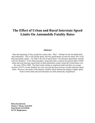
Table 5
0
20406080
0
20406080
0
20406080
0
20406080
0
20406080
0
20406080
0
20406080
1995 2000 2005 2010 1995 2000 2005 2010 1995 2000 2005 2010 1995 2000 2005 2010 1995 2000 2005 2010 1995 2000 2005 2010 1995 2000 2005 2010
Alabama Alaska Arizona Arkansas California Colorado Connecticut
Delaware Florida Georgia Hawaii Idaho Illinois Indiana
Iowa Kansas Kentucky Louisiana Maryland Massachusetts Michigan
Minnesota Mississippi Missouri Montana Nebraska Nevada New Hampshire
New Jersey New Mexico New York NorthCarolina NorthDakota Ohio Oklahoma
Oregon Pennsylvania Rhode Island SouthCarolina SouthDakota Tennessee Texas
Utah Vermont Virginia Washington West Virginia Wisconsin Wyoming
Y URBAN
RURAL
Year
Graphs by State
No real correlation can be seen between speed limits and death (it appears initially that there is
not much variation in Y, yet this is not the case – the y-axis has a wide range of numbers and
since auto fatalities (i.e. Y) are logged, they are quite close to zero). In general, the majority of
states’ auto fatality rates actually decreased over time, regardless of when the speed limits were
changed.

21
Table 6
-.5
0
.5
1
-.5
0
.5
1
-.5
0
.5
1
-.5
0
.5
1
-.5
0
.5
1
-.5
0
.5
1
-.5
0
.5
1
1995 2000 2005 2010 1995 2000 2005 2010 1995 2000 2005 2010 1995 2000 2005 2010 1995 2000 2005 2010 1995 2000 2005 2010 1995 2000 2005 2010
New Jersey New Mexico New York North Carolina North Dakota Ohio Oklahoma
Oregon Pennsylvania Rhode Island South Carolina South Dakota Tennessee Texas
Y CHANGE URBAN
CHANGE RURAL
Year
Graphs by State
Above is the depiction of fatalities and the dummy variables changerural and changeurban over
time. The variation in fatalities is now much more visible, since the range of the y-axis is
considerably smaller. However, the correlation between Y and the two variables also appears to
be difficult to distinguish. The state of Michigan has an interesting jump in fatalities in 1995, yet
this jump occurred prior to the change to higher speed limits. What is generally observable is the
distinct negative trend of auto fatalities over time, regardless of the increase in urban and rural
speed limits nationwide.

22
Table 7
-.5
0
.5
1
-.5
0
.5
1
-.5
0
.5
1
-.5
0
.5
1
-.5
0
.5
1
-.5
0
.5
1
-.5
0
.5
1
1995 2000 2005 2010 1995 2000 2005 2010 1995 2000 2005 2010 1995 2000 2005 2010 1995 2000 2005 2010 1995 2000 2005 2010 1995 2000 2005 2010
New Jersey New Mexico New York NorthCarolina NorthDakota Ohio Oklahoma
Oregon Pennsylvania Rhode Island SouthCarolina SouthDakota Tennessee Texas
Y drive 16 and up
Year
Graphs by State
As can be seen, only two states (Hawaii and Lousiana) changed the age level for issuing regular
driving licenses within the time frame of interest. The effect of Lousiana’s change to 16 is not
clearly observable, while auto deaths in Hawaii seem to depict a clear negative trend once the
state made the switch (although we cannot say for certain that this switch was the cause behind
the decline). Another point of notice is that the fatality rates of states that allow the issuance of
regular licenses to individuals under the age of 16 are not on average significantly different from
those of the other states, implying perhaps that the age of driver license issuance is not a major
factor in causing automobile fatalities.

23
Table 8
-.5
0
.5
1
-.5
0
.5
1
-.5
0
.5
1
-.5
0
.5
1
-.5
0
.5
1
-.5
0
.5
1
-.5
0
.5
1
1995 2000 2005 2010 1995 2000 2005 2010 1995 2000 2005 2010 1995 2000 2005 2010 1995 2000 2005 2010 1995 2000 2005 2010 1995 2000 2005 2010
New Jersey New Mexico New York North Carolina North Dakota Ohio Oklahoma
Oregon Pennsylvania Rhode Island South Carolina South Dakota Tennessee Texas
Y BAC LAW
Year
Graphs by State
Nearly all states’ fatality rates decreased after the BAC law was put into effect, yet auto deaths
across the country also appeared to be decreasing regardless. Perhaps we may hypothesize that
the BAC law expedited this decline. However, the auto fatality rates of several states (i.e.
Indiana, Iowa, Kentucky, and Louisiana to name a few) actually increased or stayed the same
after the BAC law was implemented. Thus the ultimate effect of the BAC law on auto deaths
when looking at the above Table remains a bit unclear.

24
Table 9
0
.2.4.6.8
1
1995 2000 2005 2010
Year
Y Baclaw
Average values of Y and baclaw across the country – we can certainly see no real change in the
decreasing trend of auto deaths, after the averaged year the law was implemented nationwide.

25
Table 10
0
.2.4.6.8
1
1995 2000 2005 2010
Year
Y Changeurban
Average values of Y and changeurban – as in the previous graph, there is no discernable change
in the decreasing trend of auto fatalities after higher urban speed limits were implemented
nationwide.

26
References
(1). Beck, Nathaniel and Jonathan Katz. “What To Do (And Not To Do) With Time-Series
Cross-Section Data,” The American Political Science Review (1995).
(2). Bond, Stephen. “Dynamic Panel Data Models: A Guide to Micro Data Methods and
Practice.” Institute for Fiscal Studies, Oxford University (2002).
(3). Bureau of Justice Statistics
(http://bjs.ojp.usdoj.gov/dataonline/Search/EandE/state_exp_next.cfm)
(4). Chan, K.S., and Johannes Ledolter. "Evaluating the Impact of the 65 mph Maximum
Speed Limit on Iowa Rural Interstates." American Statistician 50.1 (1996): 79-85.
(5). De Hoyos, Rafael and Vasilis Sarafidis. “Testing For Cross-Sectional Dependence In Panel-
Data Models.” The Stata Journal (2006).
(6). Dougherty, John. Introduction to Econometrics. Oxford University Press (2006).
(7). Dranove, David. “Fixed Effects Models.” Northwestern University
(http://www.kellogg.northwestern.edu/faculty/dranove/htm/dranove/coursepages/Mgmt%20469/
Fixed%20Effects%20Models.pdf)
(8). Dricoll, John and Aart Kraay. “Consistent Covariance Matrix Estimation With Spatially
Dependent Panel Data," The Review of Economics and Statistics, MIT Press (1998).
(9). Federal Reserve Bank of Dallas. “Smoothing Data with Moving Averages.”
(http://www.dallasfed.org/data/basics/moving.html)
(10). Hoechle, Daniel. “Robust Standard Errors For Panel Regressions With Cross–Sectional
Dependence.” The Stata Journal (2007).
(11). Insurance Institute for Highway Safety. IIHS-HLDI: Crash Testing & Highway Safety
(1998).
(12). Kezdi, Gabor. “Robust Standard Error Estimation In Fixed-Effects Panel Models.”
Budapest University of Economics (2003).
(13). Moore, Stephen. "Speed Doesn't Kill: The Repeal of the 55-MPH Speed Limit." Cato
Institute (1999).
(14). Morrison, Gail. "Repealing the 55 MPH Speed Limit." LewRockwell.com. N.p., 28
Jul 2000.
(15). New York State Department of Motor Vehicles (http://www.nydmv.state.ny.us/stats.htm),
(http://www.nydmv.state.ny.us/dmvfaqs.htm#tickets)

27
(16). Peltzman, Sam. "The Effects of Automobile Safety Regulation." The Journal of
Political Economy, 1975, 83(4), pp. 677-726.
(17). Reyna-Torres, Oscar. “Panel Data Analysis; Fixed and Random Effects.” Princeton
Unversity (http://dss.princeton.edu/training/Panel101.pdf)
(18). Woolley, John. "Statement on Signing the Emergency Highway Energy Conservation
Act." The American Presidency Project. Gerhard Peters, 02jan1974.
(19). "Fatality Analysis Reporting System (FARS)." www.nhtsa.gov/FARS. National
Highway Traffic Safety Administration, Nov 2010.
(20). "National Highway System Designation Act." U.S. Department of Transportation,
Federal Highway Administration. N.p., Dec 1995.
(21). Yaffee, Robert. “A Primer for Panel Data Analysis.” New York University (2003).

Thesis - FINAL PAPER

Recommended

Recommended

More Related Content

What's hot

What's hot (6)

Viewers also liked

Viewers also liked (11)

Similar to Thesis - FINAL PAPER

Similar to Thesis - FINAL PAPER (20)

Thesis - FINAL PAPER