1. 1
General deterrence of drinking and driving: an evaluation of the
effectiveness of three Ontario countermeasures
Qing Wu, M.Sc., Tracy Chen, M.A.Sc., Patrick A. Byrne, Ph.D., Jacob Larsen, M.U.P., Yoassry Elzohairy, Ph.D.
SafetyPolicy and Education Branch,Road User Safety Division, Ministry of Transportation Ontario, 1201
Wilson Avenue, Toronto, Ontario, M3M 1J8, Canada
Abstract
Objective:Thisworkwas conductedto evaluate the generaldeterrenteffectsof three Ontario drinking-
and-driving programs: the Administrative Driver’s Licence Suspension (ADLS), the remedial measures
program Back on Track (BOT), and Ignition Interlock (II).
Method: Both interrupted and forecasted time series analyses were used to evaluate each program.
Specifically, we asked whether the implementation of each of the three programs led to decreases in
the numbersof drinkingdriversinvolvedinfatal andinjurycollisions,andinthe numberof fatalities and
injuries resulting from drinking-and-driving related collisions in Ontario. Such a finding for any of the
three programswouldindicate thatthose program(s) actedasa general deterrent againstdrinking-and-
driving.
Results:The interruptedtime series analysisshowedthatintroductionof ADLShadsignificanteffects on
the number of drinking-and-driving related fatalities and major injuries. The forecasted time series
analysiscorroboratedthisfinding, thus providing a high degree of confidence that ADLS is an effective
countermeasure. Unlike the interrupted time series analysis, the forecasting model also showed a
significanteffectof ADLSonthe numberof alcohol-impaireddriversinvolved in collisions, as well as on
drinking-and-driving related fatalities and injuries in general. This disagreement between the two
models is not surprising given that both models use the available data quite differently and make
different assumptions. Agreement between the two models should therefore only be expected for
robusteffects.The interruptedtime seriesanalysisalsoshowedthatthe IIprogramreducedthe number
of alcohol-related fatalities and injuries. BOT did not appear to produce any general deterrent effect.
Conclusions:Of the three programsevaluated, ADLShadthe mostrobust general deterrenteffect,while
the II program appearsto have beneficial effectsaswell. The effect of ADLS was strongest for reducing
fatalitiesand majorinjuriesassociatedwith drinking-and-driving,whilethe IIprogram reduced fatalities
and all injuries related to drinking-and-driving.
Introduction
Since the early1980s, the province of Ontariohas introducedseveral countermeasuresagainst drinking-
and-driving. The three programs evaluated in this study were introduced between 1981 and 2001. On
December 17, 1981, Ontario introduced an immediate roadside suspension, known as the

2. 2
administrativedriver’slicence suspension(ADLS).Thisallowed police toimmediately suspend a driver’s
licence for12 hoursif the driverwascaught drivingwitha blood-alcohol concentration (BAC) level at or
above 50mg%. This suspension was not contingent upon any criminal charge or conviction, but was
immediate and automatic. On November 29, 1996, Ontario increased the severity of the ADLS law so
that a driver caught with a BAC level over 80mg% or who refused to provide a breath sample would
have his/herlicenseimmediatelysuspendedfor90 days. Here,we evaluate the effects of transitioning
to this new ADLS law.
In September 1998, Ontario implemented the Back on Track (BOT) remedial measures program, which
provides drinking-and-drivingoffenderswithalcohol educationandtreatmentinaneffort to discourage
re-offence. Inordertobe eligibleforlicence reinstatement, drivers convicted of a drinking-and-driving
offence are required tocompleteBOT,whichis deliveredby the Centre forAddictionandMental Health
(CAMH) - a third party provider.
In December 2001, Ontario implemented the Ignition Interlock (II) program. An ignition interlock is a
device that, when installed in a vehicle, prevents impaired driving by requiring a low breath alcohol
concentration to start the engine and/or to keep the engine running. To be eligible for the program
driversmustserve the full license suspensions under the Ontario Highway Traffic Act and the Criminal
Code of Canada, and complete the required remedial measure program, which is identical to BOT, as
describedabove. Once these conditions are met,offendershave anIIconditionplaced on their driver’s
licence and can eitherdrive withthe device installed on their vehicle, or choose not to drive while the
conditionis in place. The length of the II period is dependent on the number of prior impaired driving
convictions,withfirsttime offendersreceivingaone yearIIcondition,secondtime offendersreceiving a
three year condition, and third time offenders receiving a lifetime II condition.
Researchintothe effectivenessof drinking-and-drivingcountermeasures usually focuses on one of two
types of outcome. General deterrent effects refer to a given policy or program’s capability to prevent
offenseswithinthe overall driving population. Specific deterrent effects refer to a policy or program’s
capability to prevent drivers from reoffending as a result of the punishments imposed on them for
previousoffenses.Ourresearchfocusedonevaluatingthe generaldeterrenteffectsof the three Ontario
drinking-and-driving programs discussed above.
Numerous studies have shown that ADLS countermeasures for drunk driving are highly effective
deterrents (e.g. Ross, 1987; Ross & Gonzalez, 1988; Chaloupka et al., 1993; Williams et al., 1991;
Watson,1998), possiblydue tothe swiftness andcertainty of sanctiontheyentail (Nichols & Ross, 1990;
Wagenaar & Moldonado-Molina, 2007; Macdonald et al., 2013). Some evidence suggests that the
effectiveness of ADLS is even greater than that produced by the threat of jail time (Klein, 1989). In
Ontario specifically, the 12-hour license suspension policy was shown to have small and short-term
general deterrenteffects,thereby reducingthe numberof alcohol-relatedcrashfatalities(Vingilis et al.,
1988). The 1996 ADLS policy was shown, using only short-term data, to have significant general
deterrenteffectsondriverfatalitieswithaBAC level over 80mg%, as well as on total driver fatalities in
Ontario (Mann et al., 2000, 2002; Asbridge et al., 2009). In contrast to ADLS, evaluations of remedial
education programs and ignition interlocks have tended to focus on recidivism of offenders (i.e. on

3. 3
specific effects), reflecting the design purpose of such interventions. While ignition interlocks clearly
reduce recidivism, at least while installed (e.g. Willis et al., 2009), the effects of remedial education
and/or treatment are less clear (e.g. Wells-Parker et al., 1995), although some studies suggest
effectiveness (Watson, 1998). In any case, if these programs reduce drinking-and-driving recidivism in
Ontario, then we might expect to see this reflected in the number of alcohol-related collisions in the
whole driving population (i.e. in a general effects analysis).
Before turning to methodology, we note that the effectiveness of drinking-and-driving programs is
affected by a host of factors, including overall public awareness and administrative factors related to
program implementation. For example, a policy or program could produce no significant deterrent
effects if public awareness or policy implementation strength is low. In the case of ADLS, Mann et al.
(2000) didindeedfindthatpublicawarenessof the program increased significantly after the extension
from12 hoursto 90 daysin 1996. However,we emphasizethatourevaluationforeachcountermeasure
assessesthe combinedeffectiveness of the policy itself,alongwithits public awareness campaigns, and
its implementation details.
Among the various methodologies typically employed for evaluations of general deterrence, Auto
Regressive IntegratedMovingAverage (ARIMA)-basedinterruptedtime seriesmodels (Box &Tiao, 1975)
are the mostfrequentlyusedstatistical methodinevaluatingdrinking-and-drivingpoliciesandprograms
(Wagenaar, 1995). The prevalence of these models over time-series analysis based on ordinary least-
squares (OLS) regression models comes from the complex forms of autocorrelation that can occur in
time series data. In the case of collision data, part of this autocorrelation arises from regular seasonal
variation. The autocorrelation problem can be overcome in OLS regression by introducing numerous
dummyvariables to account for seasonality, along with more complex covariance structures requiring
parameter estimation methods beyond OLS. However, ARIMA models with intervention covariates
(referredtoasARIMAXmodels) are a more natural way to performinterruptedtime series analysis and
have commonlybeenusedto evaluate the effectiveness of policy implementation (e.g. Vingilis, 1988;
Mann et al., 2002; Howard Research, 2005; Wagenaar, 2007; Asbridge et al., 2009).
METHODS
Overview
ARIMA andARIMAX-basedtime series analysis were used to evaluate the general deterrent effects of
the three drinking-and-drivingprograms discussedabove. Monthly time series of Ontario collision data
were usedtoevaluate whetherthe implementationof these programs affected the number of alcohol-
impaired drivers, the number of fatalities and all injuries related to drinking-and-driving, and the
numberof fatalitiesand major injuries related to drinking-and-driving. Two analysis approaches were
used to answer these questions. The first was an interrupted time series approach in which ARIMAX
modelswithintervention covariates (dummies) were fit to the entire time series, covering the period
between January 1988 and December 2010. The strength of this method is that the statistical model
assesses the question of interest based upon the entire dataset, while its weakness is that specific
intervention covariate forms must be assumed. The second approach was a forecasting one in which

4. 4
ARIMA modelswithoutcovariateswerefittothe pre-intervention time series, which ran to the date at
whichthe interventionbecame effective, andsubsequently usedtoforecastpost-interventiondata. The
strength of this method is that no assumptions about intervention covariates are requires, while its
weakness is that it does not make full use of the available data. By choosing two approaches with
different strengths and weaknesses, we can be more confident that when both methods agree, the
result is trustworthy. IBMSPSS Forecasting (version 21) was the main platform for modelling.
Data
Outcome measure time series
The primary data source for the time series data, or dependent variables, in the models was the
Accident Data System (ADS) maintained by the Ontario Ministry of Transportation. As the ADLS, BOT,
and IIprograms were implemented in November 1996, October 1998 and December 2001 respectively,
data from the period between January 1988 and December 2010 were used to ensure a large time
window over which background collision trends could be estimated.
The outcome measureschosenfortime seriesanalysis were:1) the numberof alcohol-impaireddrivers
involvedincollisions, 2) the numberof fatalitiesand allinjuriesrelatedto drinking-and-drivingcollisions,
and 3) the numberof fatalitiesand majorinjuriesrelatedto drinking-and-drivingcollisions.Fatalities
were definedaspersonskilledimmediatelyorwithin30daysof the motor vehicle accident.Major
injurieswere definedaspersonsadmittedtothe hospital,includingthose admittedforobservation.
Drinking-and-drivingcollisionswere definedascollisionswhereatleastone driverinthe collisionwas
deemedtobe impairedbyalcohol,eitherviaaroadside breathtest,hospital bloodtesting,orvia
behavioural testing.
The way inwhicha driverisdeterminedtobe impairedbyalcohol inacrash situationvariesdepending
on the state of the driver.Some fractionof impaireddriverswillnotbe foundtobe so because
emergencymedical treatmentmusttake precedence overBACtesting.Alternatively,the involvedpolice
officer(s) mightnotsuspectimpairment.Therefore,one mightreasonablyquestionourcombiningof
fatalitiesandinjuries,orof fatalitiesandmajorinjuries since driversineachof these categorieswill
likelyhave impairmentdeterminedindifferentways.However,inordertoassessanyeffectof an
intervention,all thatmattersisthatprocessestypicallyemployedtoascertainthe presence of
impairmentremainconstant overthe time periodof interest andthatthey do not interactwiththe
intervention.Toourknowledge,nosystematicprocedural changesoccurredduringthe time period
studiedinOntario,aside fromintroductionof the drinking-and-drivingcountermeasures of interest.
The particularoutcome measuresdescribedabove were chosenbecause the firstishighly generalin
that itcaptures all typesof collisionsandweightscollisionswithtwoimpaireddriversmore heavilythan
those witha single suchdriver. Itcan be thoughtof as a proxyfor how manydangerouslyalcohol-
impaireddriversare onthe road.The secondmeasure excludesalcohol-relatedcollisionsthatinvolve
onlypropertydamage,andmeasuresdirectlyhow manypeople are beingphysicallyhurtasa resultof
drunkdriving.The thirdmeasure narrowsthisgroupdownfurtherbyexcludingminorinjuries,thereby
providingthe mostimportantindicatorof alcohol-relatedroadsafety.Thislattergroupmightalsobe

5. 5
more indicative of the numberof heavilyimpaireddriversonthe roadat any time,althoughwe donot
testthisassumption.
We are interested primarilyinwhetherthe three drinking-and-driving countermeasures (ADLS, BOT, or
II) cause any change in the time course of the outcome measure described.However, other factors may
impact the prevalence of drinking-and-driving and resultant fatalities and injuries during any given
period.These include1) othertransportationpoliciesimplementedduringthe same period,2) economic
phenomena, 3) demographic trends, 4) strengthened police enforcement, 5) weather, 6) alcohol
consumption levels, and others. Non-alcohol-related factors, like 1) to 5), can be controlled for by
creating a ratio time series in which the numerator is the series of interest and the denominator is a
seriesthatshouldbe affectedbyconfoundsinthe same wayasthe numerator.For example, a decrease
inthe numberof alcohol-relatedfatalitiesandinjuriesmay be due to the general deterrent effects of a
drinking-and-driving countermeasure, but it may also be due to a decrease in the number of vehicle
kilometres traveled resulting from a depressed economy. This latter factor should affect non-alcohol-
relatedfatalitiesandinjuriesinthe same directionandmagnitude as alcohol-related ones. As such, the
ratioof the two shouldremainunaffectedbychanges in total driving, but not by alcohol-related policy
changes. Therefore, our final analysis was performed on the following three time series:
 The monthly ratio of alcohol-impaired drivers involved in fatal and injury collisions in Ontario
duringthe studyperiodtonon-impaireddriversinvolvedinfatal and injury collisions in Ontario
during the study period;
 The monthlyratioof fatalities and all injuries resulting from collisions related to drinking-and-
drivingtofatalitiesand allinjuriesresultingfromnon-drinking-and-driving collisions in Ontario
during the study period; and,
 The monthly ratio of fatalities and major injuries resulting from collisions related to drinking-
and-drivingtofatalitiesand majorinjuriesresultingfrom non-drinking-and-driving collisions in
Ontario during the study period.
Each of the three time serieswaslogtransformedbefore ARIMA modellingtostabilize variance,whichis
necessary to meet the ARIMA stationarity requirements.
Time Series Covariates
The interrupted time series models (ARIMAX) involved three policy intervention variables, one
representingeachprogram.Three interventioneffecttypeswere modelledfor each policy intervention
variable: a sudden permanent effect, a sudden temporary effect, and a gradual effect. The sudden
permanenteffectwasmodeledasaHeaviside stepfunction, transitioning from zero to one at the time
of the intervention; the sudden temporary effect was modelled as a rectangular step function
transitioning from zero to one at the time of the intervention and from one to zero either two or four
yearslater;and the gradual effectwasmodeledasalinearramp originatingatintervention time. These
interventioncovariates were introduced into the ARIMAX models via a zeroth order transfer function.
Since alcohol consumption trends may affect the three outcome measures listed above, we used
Ontariomonthlyalcohol salesvolumesinthe study period as a covariate of the interrupted time series

6. 6
ARIMAXmodels.Annual alcohol sales data in Ontario, provided by the Liquor Control Board of Ontario
(LCBO), was used to generate the monthly time series of Ontario alcohol sales volume. This data was
found to be consistent with similar data from Statistics Canada.
Model fitting
All data modelingwasbasedonseasonal ARIMA(X)(p,d,q)(sp,sd,sq) modelsasimplementedinIBMSPSS
Forecasting(Version21). InthisnotationX referstotime-varyingcovariates,includingthe intervention
variables;p,d,and q are the numberof autoregressive terms,the degree of differencing,andthe
numberof movingaverage terms,respectively;andsp,sd,and sq are the seasonal equivalents.
For boththe interruptedand forecastingapproaches,ARIMA(p,d,q)(sp,sd,sq) models werefirstfitto the
pre-intervention data of each of the three log transformed time series using SPSS Expert Modeller,
producing three “pre-intervention” models. In the interrupted time series approach these pre-
intervention fits were used simply to estimate model complexity (i.e. model order) by providing the
optimal numberof (seasonal) autoregressiveterms,(seasonal) movingaverage terms,andthe degree of
(seasonal) differencing(i.e.,valuesof p,d,q, etc.). For example, the best fit pre-intervention model for
the ratio of alcohol-impaireddriversversusnon-impaireddriverswasARIMA(0,1,1)(0,1,1).Thereforethe
corresponding ARIMAX model fit to the entire time series was initially chosen to be
ARIMAX(0,1,1)(0,1,1),where the covariates,X,includedthe interventionvariables,representing each of
the three programs, and the alcohol sales time series.
The fitting procedure for the interrupted time series analysis was performed as follows: First, three
ARIMAX models, one with sudden permanent intervention covariates, one with sudden temporary
covariatesandone withgradual covariateswere fitto the entire data range from one of the three time
series(e.g.ratioof alcohol-impaireddriverstonon-impaired drivers) using the pre-intervention model
order(p,d, q, etc) determinedfor that series. Thus, a total of nine models were fit: three intervention
covariate types X three outcome time series. For each of the three models fit to each time series, the
Ljung-Box Qstatisticwascheckedto determineif the model successfullyremoved autocorrelation from
the residuals.If not,the model orderswere adjusted manually in order to achieve proper fit. Next, the
model withthe lowestBayesianInformationCriterion (BIC) was chosen to represent the time series of
interest(i.e.sudden permanent, sudden temporary, or gradual). Since the intervention covariates are
not orthogonal, a backward elimination procedure was employed in which the intervention covariate
withthe highestnon-significantp-valuewasremovedfromthe model before re-fitting. This procedure
was repeated until further removal would either: 1) eliminate a statistically significant intervention
variable, 2) worsen(increase) the BIC,or 3) produce a model with no remaining intervention variables.
By repeating the fitting procedure for all three time series, one final model was produced for each.
For the forecasting approach, the actual coefficients of the pre-intervention ARIMA(p,d,q)(sp,sd,sq)
model terms were retainedsothatdetailedpredictionsforthe post-intervention period could be made
and comparedto the actual observeddata.Significantdifferencesbetweenthe twoshould,in principle,
reveal programeffectsandallowfora direct estimationof the magnitude of the effect of the program.
Giventhe quasi-experimental design, it is always possible that some other unknown factor could also
produce differences.

7. 7
RESULTS
The raw collisionrate ratiodata correspondingtothe three outcome measuresof interest,asdescribed
above, are shownas time seriesinFigures1-3(dashedblue curves).
Pre-intervention fitting
ARIMA modelswere firstfittothe three log-transformed outcome time series for the period between
January 1988 and November 1996 (the date of ADLS introduction). For these 'pre-ADLS' models, SPSS
ExpertModellerselectedARIMA(0,1,1)(0,1,1) asthe bestfitmodel forthe logdriverratiomodel and the
log fatality and injury ratio model, and ARIMA(0,0,1)(0,1,1) for the log fatality and major injury ratio
model.Table 1showsthe model fitstatistics. The Ljung-Box Q statistic shows that the selected models
were adequately able to account for the majority of autocorrelation in each of the time-series.
The pre-ADLS models appear to de-trend and de-correlate the pre-ADLS data properly and, as such,
form an appropriate initial guess for the complexity (order) of the ARIMAX interrupted time series
analysisof all three interventions(ADLS,BOT,andII).These modelscanalso be useddirectly to perform
the forecasting analysis for the ADLS program.
In order to test for the general deterrent effects of BOT using a forecasted time series approach, a
proper model of the pre-BOT data covering the interval from January 1988 to October 1998 is required
so that extrapolationscanbe made.However,duringthistime the ADLSintervention was introduced. If
the ADLS program causeda suddenshiftinsome propertyof the time series, then the series would not
be stationary,therebyviolatingARIMA assumptions. Indeed, when we attempted to fit the three time
series of interest on the pre-BOT data, the Ljung-Box Q statistics were significant for two series (the
driver ratio and the fatalities and injuries ratio) and marginal for one series (the fatalities and major
injuries ratio series). This indicates that a simple ARIMA model without covariates could not fully
account for the full pre-BOT time series. As expected, similar results held for the II intervention.
Therefore, we used interrupted time series analysis to evaluate the effectiveness of all three
interventions, but the forecasting approach was only applied to the ADLS intervention.
Interrupted time series analysis
The interrupted time series ARIMAX models were initially assigned the same orders (number of
autoregressive terms, degree of differencing, etc.) as the pre-ADLS models, but were fit to the set of
time series data covering the entire study period (January 1988 – December 2010). The tested
covariates for each model included:
 ADLS intervention variable
 BOT intervention variable
 II intervention variable
 Ontario alcohol consumption volume estimates
Three intervention effect types (sudden permanent, sudden temporary, and gradual permanent, as
described above) were tested for each of the three policy interventions.

8. 8
For the ratio of alcohol-impaired drivers to non-impaired drivers, three ARIMAX(0,1,1)(0,1,1) models
were fit, one for each form of intervention covariates. All three models failed the Ljung-Box Q test
(p<0.00005 for all models), indicating that the pre-intervention derived models were not of sufficient
complexity, even with the addition of covariates, to account for the autocorrelation in the full time
series. SPSS Expert Modeller was also unable to find a model with appropriate order that included
covariatesandcouldpass the Ljung-Box Qtest. Manual adjustment indicated that ARIMAX(5,1,0)(0,1,1)
was the simplestmodel formthatwouldadequatelyfitthe data,withthe gradual interventioncovariate
model having the lowest BIC. None of the interaction covariate coefficients for this full model were
found to be significant, and reduction through backward elimination left no covariates in the reduced
model. This implies either that the interventions had no effect on this time series or that the optimal
model was not found.
For the ratio of fatalitiesandinjuriesresultingfrom drinking-and-drivingcrashestofatalitiesandinjuries
resultingfromnon-drinking-and-drivingcrashes,three ARIMAX(0,1,1)(0,1,1) modelswere alsofit.Again,
none passedthe Ljung-Box Qtest(p<0.005 for all models) andSPSS Expert Modeller was unable to find
an appropriate model order to adequately account for the time series autocorrelation. Manual
adjustmentindicatedthatARIMAX(3,1,1)(0,1,1) wasthe simplestmodel form that would adequately fit
the data, with the gradual intervention covariate model having the lowest BIC. No intervention
covariates were significant in the full model, but after backward elimination both ADLS and II were
foundto have significanteffects(p= 0.00014 and 2x10-6
, respectively),withADLS causing an increase in
drinking-and-driving related fatalities and injuries and II causing a decrease. The II effect is in the
expected direction, but the ADLS effect seems counterintuitive. However, there is likely a
straightforward explanation, which is discussed further in the conclusions.
For the ratio of fatalitiesandmajorinjuriesresultingfrom drinking-and-driving crashes to fatalities and
majorinjuriesresultingfromnon-drinking-and-drivingcrashes,three ARIMAX(0,0,1)(0,1,1) models were
fit.The suddentemporaryandsuddenpermanentmodels passed the Ljung-Box Q test, but the gradual
model did not (p=0.026). However, simply adding one order of autoregression, thereby producing
ARIMAX(1,0,1)(0,1,1) models,yieldedthree modelsthat all passed the Ljung-Box test and all had lower
BIC values than their ARIMAX(0,0,1)(0,1,1) counterparts. Of these new models, the one with sudden
permanenteffect interventioncovariateshad the lowest BIC value and was selected as the final model
for thistime series.Afterbackwardeliminationthe ADLSandIIcoefficientswere found to be significant
(p = 0.035 and 0.007, respectively), with ADLS decreasing the number of alcohol-related fatalities and
majorinjuries,andIIincreasingthe number. The former finding is as expected, but the latter finding is
counterintuitive. One possible explanation is that ADLS actually had a temporary effect that lasted
longerthanthe four yearswe originallymodeled.The fittingalgorithmcouldhave artificiallyconstructed
such a covariate by adding the permanent ADLS and II covariates together in the right combination. In
orderto testthis,we createda sudden temporaryADLSeffectcovariate with a five year instead of four
year width and then re-fit the sudden temporary model using this new covariate. Consistent with our
interpretation,this new model had a lower BIC than the full sudden permanent effect model. The full
version of this new model had a significant ADLS effect (p = 0.038). After backward elimination, the
reducedmodel alsoshowed asignificantADLSeffect(p= 0.009), but noeffectsof either BOT or II. Thus,

9. 9
we conclude thatADLS was responsible fora significantreductioninalcohol-relatedfatalities and major
injuries.
Forecasted time series analysis
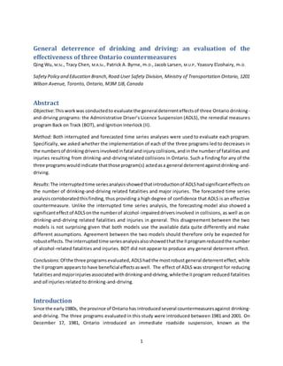
The forecastedmonthlynumbersof alcohol-impaireddriversanddrinking-and-driving related fatalities
and injurieswere calculated using the forecasted log ratios from the pre-intervention ARIMA models,
the observednumbersof non-impaireddrivers,andnon-alcohol-relatedfatalitiesandinjuries. Figures1,
2, and 3 provide graphic comparisons between the forecasted and observed values based on the
calculations (red curves).
For the logdriverratio model andlogfatalityandinjuryratiomodel,forecastedvalueswere higher than
observedvaluesonaverage forthe first4 to 5 years post implementation. The differences diminished
overtime andevenreversedafterafewyears.Thisindicatedthatthe implementation of ADLS reduced
the numbersof alcohol-impaireddriversanddrinking-and-drivingrelatedfatalitiesandinjuries,but only
for a certain period (i.e. 4 to 5 years). However, for the log fatality and major injury ratio model, the
forecastedvalueswereconsistentlyhigherthanthe observedvaluesoverthe entire studyperiod,which
indicated ADLS had long-term general deterrent effects on reducing drinking-and-driving related
fatalities and major injuries.
The model results showed (t-test p < 0.001 for each model and each forecasting period):
 For the firstfourforecastingyears(December1996 – November2000), an average of 25 fewer
alcohol-impaireddrivers permonth were involvedinfatal andinjurycollisionsevery afterADLS
implementation;
 For the firstfourforecastingyears(December1996 – November2000), an average of 47 fewer
fatalities and injuries per month resulted from drinking-and-driving collisions after ADLS
implementation; and
 For the entire forecasting period (December 1996 – December 2010), an average of 20 fewer
fatalitiesandmajorinjuries permonthresulted fromdrinking-and-drivingcollisions after ADLS
implementation.
Comparison between interrupted and forecasted time series analysis
The two time seriesapproaches used in this study produced different results regarding the number of
alcohol-impaireddriversinvolvedinfatal andinjurycrashes.The forecasting approach requires that the
pre-intervention model adequately capture all of the information within the data, aside from
intervention effects. Given that the model fit to the full range of data had to be switched from
ARIMAX(0,1,1)(0,1,1) toARIMAX(5,1,0)(0,1,1) inorderto satisfythe Ljung-Box Q test, it could simply be
that the pre-interventionmodel wasnotappropriate for forecasting.Thisis also a likely explanation for
the disagreement between the two approaches when examining the alcohol-related fatalities and
injuries time series.Whenexaminingthe time seriesof fatalities and major injuries related to drinking-
and-driving, the pre-intervention model required very little modification to fit the full data set.
Interestingly,itisfor this last time series that both analysis approaches are in full agreement. As such,

10. 10
we conclude that the estimate of the ADLS-induced reduction in alcohol-related fatalities and major
injuries generated using the forecasting analysis is trustworthy.
CONCLUSIONS
ARIMA-based interrupted and forecasted time series models were used to evaluate the general
deterrent effect of three Ontario drinking-and-driving programs; Administrative Driver’s Licence
Suspension(ADLS),BackonTrack (BOT),andIgnitionInterlock(II).The modelswere designed to answer
the following questions:
 How effective were the programs in reducing the number of alcohol-impaired drivers?
 How effective were the programsinreducingfatalitiesandinjuriesresulting from drinking-and-
driving crashes?
 How effective were the programs in reducing fatalities and major injuries resulting from
drinking-and-driving crashes?
To answer these questions, three time series were analyzed in the models:
 The monthly ratio of alcohol-impaired drivers involved in fatal and injury collisions in Ontario
duringthe studyperiodtonon-impaireddriversinvolvedinfatal and injury collisions in Ontario
during the study period;
 The monthly ratio of fatalities and injuries resulting from collisions related to drinking-and-
driving to fatalities and injuries resulting from non-drinking-and-driving collisions in Ontario
during the study period; and,
The monthlyratioof fatalitiesand majorinjuriesresultingfromcollisionsrelatedto drinking-
and-drivingtofatalitiesand majorinjuriesresultingfromnon-drinking-and-drivingcollisionsin
Ontarioduringthe studyperiod.
The modelsusednon-alcohol-related incidents to control for factors that affect road safety in general,
such as economic conditions, weather, and so on.
For eachtime series, bothinterruptedandforecasted time series models were applied to evaluate the
program effectiveness. Three types of program effectiveness were tested for each model; sudden
temporary, sudden permanent, and gradual permanent. The three programs and monthly Ontario
alcohol sales data were used as covariates in the interrupted models.
For the ADLS program,the interruptedtime seriesanalysisshowedasignificantreductioninthe number
of fatalities and major injuries, but an increase in the number of fatalities and injuries. Although we
cannot speak with certainty to the cause of the latter finding, one speculative explanation is that the
presence of ADLSwas inducingdriverstodrinksmallerquantitiesbefore driving,thereby increasing the
chance that they would become involved in a minor collision instead of a major one.
The forecastingmodel forfatalitiesandmajorinjuriesfoundthatADLSproducedasignificantreduction,
thusbolsteringthe finding of the interrupted time series analysis. Given this agreement between the

11. 11
two approaches, we are highly confident that ADLS reduces fatalities and major injuries. The fact that
the forecasted andinterrupted time series approachesproduceddifferingresultsforthe othertwo time
seriesismostlikelytohave arisenfrominadequate pre-interventionmodels,as described in the results
section.
The interrupted time series approach showed that the II program significantly reduced the number of
fatalitiesandinjuriesresultingfrom drinking-and-driving.Whileitispossiblethatthe IIprogram reduced
incidencesof drinking-and-drivinginthe general population,itseems likelythatitsprimaryeffectwasto
reduce incidences of drinking-and-driving by participants in the ignition interlock program. Because II
participantswithinstalledinterlockswouldnotbe able todrinkand drive in the equipped vehicles, it is
likelythatwhilethe interlockswere installed,IIparticipantswouldbe involved in fewer alcohol-related
collisions.We didnotattemptto estimate the magnitude in the reduction of alcohol-related collisions
generated by the interlock program because we were not confident that the significant effects of the
ADLS had stabilizedbythe time of the implementationof the IIprogram.This is because the best fitting
ARIMAXmodel forthe fatalitiesandmajorinjuriestime series required an ADLS intervention covariate
that affectedthe time seriesforup to five years, longer than the period between introduction of ADLS
and II. Therefore, any attempt to specifically measure the magnitude of the significant effect of the II
program would be subject to large uncertainties.
Both the forecasted and interrupted time series approaches found that the BOT program had no
significant general deterrent effects. This is unsurprising since the BOT program targets convicted
impaireddriversratherthan the general public,unlike ADLS, andBOTdoesnot activelyimpede drinking-
and-driving,asdoesthe interlockprogram.Itwouldbe more appropriate to evaluate the effectiveness
of BOT as a specific deterrent, rather than as a general deterrent.
Acknowledgements
We wishtothank our stakeholders for valuable guidance, with special thanks to Andy Murie (Mothers
Against Drunk Driving Canada), Dr. Robert Mann (Centre for Addiction and Mental Health), Robyn
Robertson(TrafficInjuryResearch Foundation),WardVanlaar (Traffic Injury Research Foundation), and
SheilaghStewart(OntarioMinistryof AttorneyGeneral). We alsowishtothankAntonio Loro and Tracey
Ma for feedback on an earlier draft of this manuscript.

12. 12
References
Asbridge, M; Mann, R.; Smart, R.; Stoduto, G.; Beirness, D.;Lamble, R.; Vingilis, E. (2009) The effects of
Ontario’s administrative driver’s license suspension law on total driver fatalities: a multiple time series
analysis, Informa Healthcare USA, Drugs: education, prevention and policy, 16(2):140-151
Box,G.E.P.and Tiao, G.C.(1975) Intervention analysis with applications to economic and environmental
problems, Journal of the American Statistical Association, 70(349):70-79
Chaloupka,F.J.;Saffer,H.;andGrossman,M. (1993) Alcohol ControlPolicies and Motor-vehicleFatalities,
Journal of legal Studies 22:161-186
DeYoung,DavidJ. (1997) An Evaluation of the Effectiveness of Alcohol Treatment, Driver License actions
and Jail Terms in Reducing Drunk Driving Recidivism in California, Addiction, 92(8):989-997
Howard Researchand Management Consulting (2005), Evaluation of the Alberta Administrative License
Suspension Program.
Klein, T.M. (1989) Changes in Alcohol-involved Fatal Crashes Associated with Tougher State Alcohol
Legislation, US Department of Transportation, National Highway Traffic Safety Administration
Macdonald,S.; Zhao,J.; Martin,G.; Brubacher,J.;Stockwell,T.;Arason,N.;Steinmetz,S.;Chan,H. (2013)
The Impact on Alcohol-related Collisions of the Partial Decriminalization of Impaired Driving in British
Columbia, Canada, Accident Analysis and Prevention, 59:200-205
Mann, R.; Smart,R.; Stoduto,G.; Adlaf,E.;Vingilis,E.; Beirness,D.;Lamble,R. (2000) Changing drinking-
and-driving behaviour: the effects of Ontario’s administrative driver’s licence suspension law, Canadian
Medical Association Journal, 162(8):1141-1142
Mann, R.; Smart,R.; Stoduto,G.; Beirness,D.;Lamble,R.;Vingilis, E. (2002) The early effects of Ontario’s
administrative driver’s licence suspension law on driver fatalities with a BAC>80mg%, Can J Public
Health. 93(3):176-80
Nichols, J. and Ross, H. (1990) The effectiveness of Legal Sanctions in dealing with drinking drivers,
Alcohol, Drugs and Driving, 6(2):33-60
Ross, H. (1987) Administrative license revocation in New Mexico: An Evaluation, Law and Policy 9(1): 5-
16
Ross, H. and Gonzales, P. (1988) Effects of License Revocation on Drunk-Driving Offenders, Accident
Analysis & Prevention, 20(5):379-391
Vingilis,E.andBlefgenH.;Lei H.; SykoraK.; andMann R. (1988) An Evaluation of theDeterrent Impact of
Ontario’s 12 Hour Licence Suspension Law, Accident Analysis & Prevention, 20(1):9-17

13. 13
Wagenaar, A.; Zobeck, T.;Williams, G.D.; Hingson, R. (1995) Methods Used in Studies of Drink-drive
ControlEfforts:A Meta-Analysisof The Literature From 1960 to 1991, AccidentAnalysis and Prevention,
27(3)307-316
Wagenaar, A. and Maldonado-Molina M. (2007) Effects of Drivers’ License Suspension Policies on
Alcohol-Related Crash Involvement: Long-term Follow-up in Forty-Six States, Alcoholism: Clinical and
Experimental Research, 31(8):1399-1406
Watson, B. C. (1998) The Effectiveness of Drink Driving Licence Actions, Remedial Programs and Vehicle-
based Sanctions, 19th
ARRB Research Conference, 66-87.
Wells-Parker, E.; Bangert-Drowns, R.; McMillen, R. and Williams, M. (1995) Final results from a meta-
analysis of remedial interventions with drink/drive offenders, Addiction, 90(7):907-926
Williams,A.;Weinberg,K.; and Fields, M. (1991) The Effectiveness of Administrative License Suspension
Laws, Alcohol, Drugs and Driving, 7(1):55-62
Willis, C.; Lybrand, S. and Bellamy, N. (2004) Alcohol ignition interlock programmes for reducing drink
driving recidivism. Cochrane Database of Systematic Reviews, Issue 3. Art. No.: CD004168

14. 14
Table 1. Pre-ADLS Model Statistics
Log Time
Series
ARIMA model
order
Model Fit statistics Ljung-Box Q(18) Number
of
Outliers
Stationary R-
squared
R-squared Statistics DF Sig.
Driver Ratio (0,1,1)(0,1,1) .497 .609 19.715 16 .233 0
Fatality/Injury
Ratio
(0,1,1)(0,1,1) .464 .565 23.975 16 .090 0
Fatality/Major
Injury Ratio
(0,0,1)(0,1,1) .303 .345 15.412 16 .495 0

15. 15
Figure captions
Figure 1: The monthly number of drunk drivers involved in collisionsisdepicted by the dashed blue curve. Clear
seasonal patterns can be seen. The red curve depicts forecasted values for the same quantity as generated by an
ARIMA model fitsolely to the pre-intervention data. The solid vertical linerepresents the date at which the ADLS
program came into effect.
Figure 2: The monthly number of fatalities and all injuries resultingfromdrinking-and-driving is depicted by the
dashed blue curve. The red curve depicts forecasted values for the same quantity, as generated by an ARIMA
model fit solely to the pre-intervention data. The solid vertical linerepresents the date at which the ADLS program
came into effect.
Figure 3: The monthly number of fatalities and majorinjuries resultingfromdrinking-and-driving is depicted by the
dashed blue curve. The red curve depicts forecasted values for the same quantity, as generated by an ARIMA
model fit solely to the pre-intervention data. The solid vertical linerepresents the date at which the ADLS program
came into effect.

16. 16
Figure 1

17. 17
Figure 2

18. 18
Figure 3