response spectra

ISET Journal of Earthquake Technology, Paper No. 475, Vol. 44, No. 1, March 2007, pp. 25–37
RESPONSE SPECTRAAS A USEFUL DESIGN AND ANALYSIS TOOL
FOR PRACTICING STRUCTURAL ENGINEERS
Sigmund A. Freeman
Wiss, Janney, Elstner Associates, Inc.
2200 Powell Street, Suite 925
Emeryville, CA 94608, U.S.A.
ABSTRACT
Although response spectra have been in general use for decades by researchers, academics, and
geotechnical professionals, their use by structural design professionals has generally been limited.
However, as response spectra and dynamic analysis are being included within the newer building codes
and as performance-based design (PBD) techniques are becoming acceptable, there is a need for the
design professional to more clearly understand the meaning and usefulness of response spectra. The
purpose of this paper is to review the concept of response spectra for design engineers not familiar with
their significance and to summarize a variety of uses that can be applied for purposes such as rapid
evaluation for a large inventory of buildings, performance verification of new construction, evaluation of
existing structures for seismic vulnerability, and post earthquake estimates of potential damage of
buildings.
KEYWORDS: Response Spectra, Building Codes, Performance-Based Design, Seismic Vulnerability,
Earthquake Intensity
INTRODUCTION
The concept of response spectra was first incorporated into the United States building codes in the
late 1950’s by means of the coefficient C in the lateral force equation V KCW= by the Structural
Engineers Association of California (SEAOC, 1960), where V is the total lateral force, K is a structural
systems coefficient of 1.33, 1.0 or 0.67, and W is the total dead load. Over the decades, response spectra
have been playing an increasing role in the development of earthquake design criteria. Much of this is due
to research and the vast data obtained from recording earthquake motion from earthquakes in California,
such as 1971 San Fernando, 1989 Loma Prieta, and 1994 Northridge, as well as from earthquakes
worldwide.
The paper traces the development of building code provisions and the relationship to response
spectra. Response spectra used for design tend to be smooth curves, whereas response spectra obtained
from ground motion recordings are generally very ragged with sharp spikes and valleys. The effects of
these differences are discussed along with recommendations on how to graphically smooth out the curves.
In general, response spectra are used to analyze structures that respond within elastic-linear limits. The
paper presents methods of using response spectra to evaluate structural response in the inelastic-nonlinear
range. This includes easy to use graphical methods that compare the seismic demand represented by a
response spectrum to the capacity of the structure represented by pushover force-displacement curves.
Such methods are the capacity spectrum method (CSM) developed by the author (Freeman et al., 1975) as
well as modifications (ATC, 1996; FEMA, 2005; Freeman, 2006), and procedures presented by others
(Fajfar, 1998; Priestley et al., 1996). Other uses of response spectra include the development of an
earthquake engineering intensity scale (EEIS) that extends the TriNet instrumental intensity scale (Wald
et al., 1999) to estimate damage levels for a variety of building types.
INTRODUCTION TO RESPONSE SPECTRA
Response spectra provide a very handy tool for engineers to quantify the demands of earthquake
ground motion on the capacity of buildings to resist earthquakes. Data on past earthquake ground motion
is generally in the form of time-history recordings obtained from instruments placed at various sites that
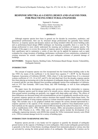
are activated by sensing the initial ground motion of an earthquake. The amplitudes of motion can be

26 Response Spectra as a Useful Design and Analysis Tool for Practicing Structural Engineers
expressed in terms of acceleration, velocity and displacement. The first data reported from an earthquake
record is generally the peak ground acceleration (PGA) which expresses the tip of the maximum spike of
the acceleration ground motion (Figure 1).
-0.5
-0.4
-0.3
-0.2
-0.1
0.0
0.1
0.2
0.3
0.4
0.5
0 1 2 3 4 5 6 7 8 9 10
Time (sec)
Acceleration(g)
Peak Acceleration
Fig. 1 Recorded ground motion (Holiday Inn, Van Nuys 1994, 270 degrees: 0–10 sec)
Although useful to express the relative intensity of the ground motion (i.e., small, moderate or large),
the PGA does not give any information regarding the frequency (or period) content that influences the
amplification of building motion due to the cyclic ground motion. In other words, tall buildings with long
fundamental periods of vibration will respond differently than short buildings with short periods of
vibration. Response spectra provide these characteristics. Picture a field of lollipop-like structures of
various heights and sizes stuck in the ground. The stick represents the stiffness (K*) of the structure and
the lump at the top represents the mass (M*). The period of this idealized single-degree-of-freedom
(SDOF) system is calculated by the equation:
1/ 2
2 ( */ *)T M Kπ= (1)
If the peak acceleration (Sa) of each of these SDOF systems, when subjected to an earthquake ground
motion, is calculated and plotted with the corresponding period of vibration (T), the locus of points will
form a response spectrum for the subject ground motion. Thus, if the period of vibration is known, the
maximum acceleration can be determined from the plotted curve. When calculating response spectra, a
nominal percentage of critical damping is applied to represent viscous damping of a linear-elastic system,
typically five-percent.
Response spectra can be plotted in a variety of formats. A format commonly used in the 1960s was
the tripartite logarithmic plot, where the vertical scale is spectral velocity (Sv) and the horizontal scale is T
in seconds or frequency (f) in Hertz. On diagonal lines are designated Sa and spectral displacement (Sd).
An example is shown in Figure 2.
Mathematical relationships between the components of response spectra are given by the following
equations:
( / 2 )v aS T Sπ= (2)
(2 / )a vS T Sπ= (3)
2
( / 2 ) ( / 2 )d v aS T S S Tπ π= = (4)
1/f T= (5)
Figure 3 shows other graphical formats used to represent response spectra. Figure 3(a) is known as
the ADRS format (Mahaney et al., 1993) that plots Sa versus Sd and shows the period, T, as radial lines.
Curved lines representing Sv can also be added (not shown, see Figure 4(b)). ADRS is essentially the

ISET Journal of Earthquake Technology, March 2007 27
tripartite format in a rotated linear coordinate system. Figure 3(b) is the commonly used Sa versus T
coordinate system. When Sd is the unit of interest, the Sd versus T format can be used (Figure 3(c)). The
relationships among these curves are consistent with the equations listed above, which define Sv as a
pseudo velocity.
1
10
100
0.1 1.0 10.0
Period T (sec)
SpectralVelocitySv(cm/sec)
Holiday Inn-Van Nuys 1994-270deg
2.0g
1.0g
0.5g
0.2g
0.05g
0.02g
0.01g
50cm
20cm
2cm
1cm
0.5cm
5cm
0.1g
10cm
Fig. 2 Tripartite (logarithmic) response spectra
The response spectra shown in Figures 2 and 3 represent the ground motion recorded at the ground
level of the Holiday Inn hotel structure during the Northridge earthquake of January 1994 in California,
U.S.A. The continuous curves represent the horizontal motion in the 0-degree direction and the dashed
curves represent the horizontal orthogonal motion in the 270-degree direction. Vertical motion was also
recorded (not shown). Ground motion, as well as building motion, was recorded for many other locations
during the Northridge event. Response spectra have also been obtained during the 1971 San Fernando
earthquake as well as from other earthquakes in the Los Angeles, California area. This data bank, as well
as data from earthquakes from all over the world, provides useful tools for studying the effects of
earthquake ground motion on building structures and for the development of code provisions for the
design of buildings.
It is observed that the response spectra shown in Figures 2 and 3 are rather jagged with sharp peaks
and valleys; and there are significant variations in the two directions of motion. It can also be shown that
there are large variations in ground motion characteristics at other sites for the same earthquake, as well
as for the same site from other earthquakes. The peaks and valleys illustrate the sensitivity of the response
of structures to a slight variation in the natural period of vibration. The large variations in ground motion
characteristics illustrate the difficulties in accurately predicting demands of future earthquakes. This leads
us to the challenge to develop standard response spectra that give a reasonable probability of having
credible design provisions.
Methods of constructing smooth response spectra for design purposes have been developed to
compensate for the peaks, valleys, and shape variations in actual response spectra; for example, the use of
a constant Sa for short periods of response, constant Sv for the mid range, and constant Sd for long period
response to develop probabilistic design spectra (Newmark and Hall, 1982; Newmark et al., 1973). An
example of smooth spectra is shown in Figure 4 based on a building code design response spectrum for a
site of high seismicity.

0.0
0.1
0.2
0.3
0.4
0.5
0.6
0.7
0.8
0.9
1.0
1.1
1.2
1.3
1.4
1.5
1.6
1.7
0 2 4 6 8 10 12 14 16 18 20 22 24 26 28 30 32 34 36 38
Spectral Displacement, Sd (cm)
SpectralAcceleration,Sa(g)
Period, T (sec)
T=0.5
T=1.0
T=1.5
T=10.0
T=4.0
T=0.75
T=2.5
0.30.2
(a)
0.0
0.1
0.2
0.3
0.4
0.5
0.6
0.7
0.8
0.9
1.0
1.1
1.2
1.3
1.4
1.5
1.6
1.7
0.0 0.2 0.4 0.6 0.8 1.0 1.2 1.4 1.6 1.8 2.0 2.2 2.4 2.6 2.8 3.0 3.2 3.4 3.6 3.8 4.0
Period, T (sec)
(b)
0
2
4
6
8
10
12
14
16
18
20
22
24
26
28
30
32
34
36
38
0.0 0.2 0.4 0.6 0.8 1.0 1.2 1.4 1.6 1.8 2.0 2.2 2.4 2.6 2.8 3.0 3.2 3.4 3.6 3.8 4.0
Period, T (sec)
SpectralDisplacement,Sd(cm)
(c)
Fig. 3 Response spectra formats (Holiday Inn, Van Nuys 1994): (a) ADRS format, (b) Sa versus
T format, (c) Sd versus T format

1
10
100
0.1 1.0 10.0
Period T (sec)
1997 UBC Zone 4 Soil Type C
S i 6
2.0g
1.0g
0.5g
0.2g
0.05g
0.02g
0.01g
50cm
20cm
2cm
1cm
0.5cm
5cm
0.1g
10cm
(a)
0.0
0.1
0.2
0.3
0.4
0.5
0.6
0.7
0.8
0.9
1.0
1.1
1.2
1.3
1.4
1.5
1.6
1.7
0 5 10 15 20 25 30 35 40 45 50 55 60
1997 UBC Zone 4 Soil Type C
Period, T (sec)
Sv = 100 cm/sec
Sv = 75 cm/sec
Sv = 50 cm/sec
T=0.5 T=1.0
T=1.5
T=10.0
T=4.0
T=0.75
T=2.5
0.30.2
Sv = 100 cm/sec
Sv = 50 cm/sec
Sv = 75 cm/sec
(b)
Fig. 4 Building code type smooth response spectra: (a) Tripartite format, (b) ADRS format
The example shown is for a 1997 Uniform Building Code criterion for seismic zone 4 at a soil
category C site. The PGA is 0.4g (i.e., 40% of gravity), the constant Sa is 2.5 times the PGA (= 1.0g).
Constant velocity is based on Sa at one second that equals 1.4 times PGA (= 0.56g). This translates to a SV
equal to 87 cm/sec (using Equation (2)). Assuming a cut-off period of 4 sec, the constant displacement
becomes 56 cm (using Equation (4)).
Once design response spectra are established, it is fairly simple to establish seismic design forces for
a building. For low-rise buildings, where the fundamental mode of vibration (in each direction) is
predominant, we estimate the period of vibration of the building and find the corresponding Sa. This may
be used as a base shear coefficient for determining the lateral forces on the building or adjustments may
be made for dynamic participation factors. For tall buildings, where the dynamic effects of higher modes
of vibration are significant, spectral accelerations for each of the several modes may be quickly
determined using the estimated periods. If the period estimates are revised, the lateral forces can be easily
adjusted proportionally to the revised spectral accelerations.

INFLUENCE OF RESPONSE SPECTRA ON BUILDING CODE PROVISIONS
The basis for the development of current seismic building code provisions had their beginnings in the
1950s. A joint committee of the San Francisco section of ASCE and the Structural Engineers Association
of Northern California prepared a “model lateral force provision” based on a dynamic analysis approach
and response spectra (Anderson et al., 1952). The proposed design curve, /C K T= , was based on a
compromise between a standard acceleration spectrum by M.A. Biot (Biot, 1941, 1942) and an El Centro
analysis by E.C. Robison (Figure 5). It is interesting to note that the PGA of 0.2g in the Biot curve has a
peak spectral acceleration of 1.0g at a period of 0.2 sec. The curve then descends in proportion to 1/T (i.e.,
constant velocity). If the peak spectral acceleration is limited to 2.5 times the PGA, the Biot spectrum is
very close to the 1997 UBC design spectrum for a PGA of 0.2g (dashed line without symbols in Figure
5). The proposed design lateral force coefficient was 0.015/C T= , with a maximum of 0.06 and a
minimum of 0.02 (line with dots in Figure 6). These values were considered consistent with the current
practice, and the weight of the building included a percentage of live load.
0.0
0.1
0.2
0.3
0.4
0.5
0.6
0.7
0.8
0.9
1.0
1.1
0.0 0.1 0.2 0.3 0.4 0.5 0.6 0.7 0.8 0.9 1.0 1.1 1.2 1.3 1.4 1.5
Period, T (sec)
Standard Acceleration Spectrum (M. A. Biot)
El Centro Analysis (Robison)
Proposed Design Curve C=K/T
1997 UBC Z=0.2, Soil Type B
Fig. 5 1952 Joint Committee Response Spectra (Anderson et al., 1952)
In 1959, the Seismology Committee of the Structural Engineers Association of California published
“Recommended Lateral Force Requirements” (generally referred to as the SEAOC bluebook) and
included “Commentary” in 1960 (SEAOC, 1960). Influenced by the Joint Committee (many of the
members were on both committees), recommendations were proposed that were adopted for the 1961
Uniform Building Code (UBC) (ICBO, 1961). The new recommended design lateral force coefficient was
1/3
0.05/C T= , and the live loads were not included in the weight (except for a percentage in storage
facilities). By using T to the one-third power, the equation could account for higher modal participation
and give a larger load factor for tall buildings. In addition it avoided the need for a minimum cut-off. The
maximum was set at 0.10C = (Figure 6). Also shown in Figure 6 is a comparably adjusted version of
the 1997 UBC.
Over the years, the SEAOC bluebook and the UBC went through many revisions, generally
influenced by some events such as the 1971 San Fernando, 1989 Loma Prieta, and 1994 Northridge
earthquakes, and by data relating to soil effects. The comparable curves shown in Figure 7 have been
adjusted to represent strength design response spectra and include factors representing soil classification
type D. At this level of design, the structures would be expected to remain linear-elastic with some
reserve capacity before reaching yield. In order to survive a major earthquake ground motion (e.g., PGA
= 0.4g) the structure is expected to experience nonlinear post-yielding response.

g ( )
0.00
0.01
0.02
0.03
0.04
0.05
0.06
0.07
0.08
0.09
0.10
0.11
0.12
0.13
0.14
0.0 0.4 0.8 1.2 1.6 2.0 2.4 2.8 3.2 3.6 4.0
Period, T (sec)
LateralForceCoefficient,C
SEAOC 1959, UBC 1961
Proposed Design Coefficient (1952), with LL
Lower limit for 1952
1997 UBC zone 4, adjusted for ASD
Lower limits for 1997 UBC
Lower limits for 1997 UBC
Fig. 6 1959 design lateral force coefficients (SEAOC, 1960)
0.00
0.05
0.10
0.15
0.20
0.25
0.30
0.35
0.0 0.5 1.0 1.5 2.0 2.5 3.0 3.5 4.0
Period T (sec)
Pre-1976 UBC
1976-1985 UBC
1988-94 UBC
1997 UBC
UBC: Cs=0.11*Ca*I
UBC: 0.8*Z*Nv*I/R
1997 UBC
1988-94 UBC
1976-85 UBC
Pre-1976
C
Fig. 7 UBC strength design response spectra (Zone 4, Soil D equivalents)—1961 to 1997
RESPONSE SPECTRA FROM GROUND MOTION RECORDINGS
It is convenient for design to have smooth response spectra; however, in the real world response
spectra come in a large variety of sizes and shapes. Therefore, data on PGA and intensity do not give the
full picture of an earthquake event. Examples of response spectra from three locations in the Los Angeles,
California area from the 1994 Northridge earthquake are shown in Figure 8. The locations are Santa
Monica, Newhall and Sylmar, which experienced PGAs greater than 0.6g (code’s maximum probable
PGAs are generally considered to be 0.4g). The ADRS format is used and, for scale, constant spectral
velocity is shown for 150 and 75 cm/sec by double-dot-dash curves. For Santa Monica the demand is
great for very short period buildings (T < 0.3 sec) and moderate for tall buildings (T > 1.5 sec). In the
mid-period range the demands are relatively small. On the other hand, Newhall has a huge demand in the
mid-period range with a broad double hump (T from 0.6 to 1.5 sec). The Sylmar spectrum has moderate

demands in the mid-period range, but has a very large displacement demand for long periods (T from 2 to
4 sec). It is tempting to envelope these and a whole family of response spectra to illustrate that the ground
motion was about twice the expected average 475-year event, but that would be misleading. For each of
the locations, buildings would respond differently, and because of energy absorption (in soil and in the
building), nonlinearity and changing periods, many buildings avoided catastrophic results.
0.0
0.2
0.4
0.6
0.8
1.0
1.2
1.4
1.6
1.8
2.0
2.2
2.4
2.6
2.8
0 5 10 15 20 25 30 35 40 45 50 55 60 65 70 75 80
Santa Monica Channel 1
Newhall-CD24279B
Sylmar Free Fld CH 3 - 0deg
Sv = 150 cm/sec
Sv = 75 cm/sec
Period, T (sec)
T=0.5
T=1.0
T=1.5
T=10.0
T=4.0
T=0.75
T=2.5
0.30.2
Sv = 150 cm/sec
Sv = 75 cm/sec
Fig. 8 Three Northridge, 1994 response spectra (5% damped)
In Figure 9, response spectra are shown for the Holiday Inn hotel structure, which experienced
damage from both the 1971 San Fernando and 1994 Northridge earthquakes. The spectra with circles
show two directions for 1994 and the curves with squares show 1971. The building experienced damage
and was softened up by the 1971 earthquake (Murphy, 1973). The initial period was about 0.5 sec; after
the earthquake it was about 1 sec. The 7-story pushover curve represents the capacity of the structure
(e.g., lateral force versus roof displacement, transformed to Sa versus Sd). The curve shown in Figure 9
was obtained by an evaluation of the recorded building motion (Gilmartin et al., 1998) and is consistent
with calculations. Figure 9(a) shows 5% damped spectra and Figure 9(b) shows 20% damped spectra. The
structure is overwhelmed by the 5% damped spectra; however, the use of 20% damped spectra to
represent inelastic-nonlinear response spectra (Freeman, 2004), illustrates how the building survived
without total collapse (i.e., the capacity curve breaks through the response spectra envelopes). In this
example 20% damping represents roughly a displacement ductility of 2.5 (Freeman, 2006).
SMOOTHING RESPONSE SPECTRA
If there is a desire to construct a smooth spectrum from a jagged response spectrum Figure 10(a)
illustrates a very simple method. Using the ADRS format, we identify the peak spectral acceleration and
draw a horizontal line (constant acceleration). We do the same for the peak spectral displacement,
drawing a vertical line for the maximum constant displacement. Then, moving out along radial lines from
the origin, we locate the maximum spectral velocity (this may be more visually clear on the tripartite
graph in Figure 10(b)). Connecting the lines forms a maximum smooth spectrum. A similar procedure is
used to form the minimum smooth spectrum (for the minimum acceleration we use the spectral
acceleration at 0.1T = sec to avoid selecting the peak ground acceleration). Taking an average of the
maximum and minimum curves will result in a reasonable estimation of a smooth spectrum. Also shown
on the Figure 10 graphs are peak ground motion (PGM) spectra, which are formed using the measured
peak acceleration, velocity and displacement. An interesting use of these graphs is to estimate dynamic
amplification factors (DAFs) by dividing spectral values by ground motion values. For example, if

average constant acceleration (1.05g) is divided by the peak ground acceleration (0.4g) the DAF is about
2.5. For velocity the DAF is about 1.7, and for displacement the DAF is about 2.3.
0.0
0.1
0.2
0.3
0.4
0.5
0.6
0.7
0.8
0.9
1.0
1.1
1.2
1.3
1.4
1.5
1.6
1.7
0 5 10 15 20 25 30 35 40 45 50
HI VN 1971 Transverse
HI VN 1971 Long
7-story pushover from instr 1971 plus 1994 envelope
Period, T (sec)
T=0.5 T=1.0
T=1.5
T=4.0
T=0.75
T=2.5
0.30.2
(a)
0.0
0.1
0.2
0.3
0.4
0.5
0.6
0.7
0.8
0.9
0 2 4 6 8 10 12 14 16 18 20 22 24 26 28
Northridge 1994 VN-1
Northridge 1994 VN-2
HI VN 1971 Transv (20%est)
HI VN 1971 Long (20%est)
7-story pushover from instr 1971 plus 1994 envelope
Period, T (sec)
T=0.5 T=1.0
T=1.5
T=4.0
T=0.75
T=2.5
0.30.2
(b)
Fig. 9 Holiday Inn, Van Nuys response spectra for 1971 and 1994 earthquakes: (a) 5% damped,
and (b) 20% damped

0.0
0.2
0.4
0.6
0.8
1.0
1.2
1.4
1.6
1.8
0 2 4 6 8 10 12 14 16 18 20 22 24 26 28 30 32 34 36 38 40
PeakRS
Avg of min;max
MinRS
PGM Gd-00
Period, T (sec)
T=0.5
T=1.0
T=1.5
T=10.0
T=4.0
T=0.75
T=2.5
0.30.2
(a)
1
10
100
0.1 1.0 10.0
Period T (sec)
PeakRS
Avg of min;max
MinRS
PGM
2.0g
1.0g
0.5g
0.2g
0.05g
0.02g
0.01g
50cm
20cm
2cm
1cm
0.5cm
5cm
0.1g
10cm
(b)
Fig. 10 Smoothing response spectra and ground motion spectra (Holiday Inn, Van Nuys 1994):
(a) ADRS format, (b) Tripartite format
AN EARTHQUAKE ENGINEERING INTENSITY SCALE
Emergency response after an urban area earthquake requires incorporation of data from various
sources. Main sources of data for engineering use are the so-called free-field instruments, as used in
TriNet ShakeMap, and strong-motion instruments installed in buildings. The TriNet system is capable of
providing a rapid instrumental intensity map for strong motion earthquakes on the basis of an array of
recording instruments. The instrumental intensity scale (Imm) is based on recorded peak ground
accelerations (PGAs) and peak ground velocities (PGVs). Both are calibrated against historical Modified
Mercalli Intensity (MMI) data, and are related to two parallel scales describing potential damage and
perceived shaking (Wald et al., 1999). To improve emergency response, an Earthquake Engineering
Intensity Scale (EEIS), built on a scale initially developed by the late John A. Blume in 1970s (Blume,
1970), is presented (Freeman et al., 2004). EEIS allows translation of ground shaking information in the
form of response spectra at a site into response/shaking intensity for different kinds of buildings. When
this translation is presented in Acceleration-Displacement Response Spectrum (ADRS) format, spectrum

levels for different period ranges can be graded into various EEIS levels by relating them to the
Instrumental Intensity (Imm) scale developed for TriNet ShakeMap.
To construct the link, response spectra corresponding to the Imm scale can be approximated by
applying dynamic amplification factors to the TriNet PGA and PGV values. Studies dating back from the
1970s to the present have provided recommendations for these amplification factors (Newmark et al.,
1973; Newmark and Hall, 1982). By multiplying the PGA values by the acceleration amplification factor
for the short periods (i.e., constant acceleration range) and by multiplying the PGV values by the velocity
amplification factor for the medium-to-long periods (i.e., constant velocity range), smooth response
spectra can be formed into a structural response intensity scale. Amplification factors of 2.0 for the PGA
and 1.7 for the PGV were selected as illustrated in Figure 11. The response spectra shown in Figure 8 are
shown superimposed on transformed Imm scales VII through X. Note that they have small bumps into X,
but generally lie in intensity IX. Santa Monica lies in intensity VIII except at very short periods. The
EEIS is also shown on the tripartite format (Figure 11(b)). Note the period bands that designate zones of
short-, medium- and long-period buildings.
0.0
0.4
0.8
1.2
1.6
2.0
2.4
2.8
0 4 8 12 16 20 24 28 32 36 40 44 48 52 56 60 64 68 72 76 80
Newhall Chl 3
Sylmar Chl 3
Santa Monica Chl 1
T
Series3
T=0.5 T=1.0
T=1.5
T=10.0
T=4.0
VIII
VII
IX
X
T=0.75
T=2.5
0.30.2
Sylmar
Newhall
Santa Monica
(a)
10
100
1000
0.1 1.0 10.0
Period T, sec
SpectralVelocitySv(cm/s)
Newhall Chl 3
Sylmar Chl 3
Santa Monica Chl 1
T-Bands
S- S S+ M- M M+ L- L L+
X
IX
VIII
VII
VI VI
VII
VIII
IX
X
(b)
Fig. 11 Earthquake Engineering Intensity Scale (EEIS): (a) ADRS format, (b) Tripartite format

CLOSING
An introduction to response spectra has been presented, illustrating procedures that may be useful to
professional engineers as an aid to design and evaluation of buildings and other structures. When
earthquake ground motion data is available, the use of response spectra can be very useful in
understanding how buildings perform and to identify deficiencies and damage potential.
However, response spectra, as in any other technique, must be used with caution and a good
understanding of the process. For single-degree-of-freedom systems responding in a linearly elastic
manner, response spectra give good credible results, assuming that the data is credible. For a measured
earthquake response spectrum with sharp peaks and valleys, the variations due to uncertainty in actual
structural period of vibration is visually apparent. For multi-modal systems, the combination of modes is
generally done by SRSS (square root of the sum of the squares) or CQC (complete quadratic
combination) rule. Although these rules are based on probability approximations, the results are generally
reasonable. The more technical time-history method is generally considered more exact; however, due to
sensitivity to small variations in accuracy of structural periods of vibration, there are also uncertainties in
this procedure. When analysis is extended into the inelastic nonlinear realm of structural response,
complexities of analysis multiply. Response spectrum techniques allow engineers to visually imagine how
buildings will perform during major damaging earthquakes.
It is recommended that researchers and design professionals put more effort into detailed
examinations of individual building response records. By deconstructing individual recorded floor
motions into individual modes of vibration, there is the potential of better understanding how buildings
perform during earthquake ground motions. This could lead to developing better methods of using
response spectra.
REFERENCES
1. Anderson, A.W., Blume, J.A., Degenkolb, H.J., Hammill, H.B., Knapik, E.M., Marchand, H.L.,
Powers, H.C., Rinne, J.E., Sedgwick, G.A. and Sjoberg, H.O. (1952). “Lateral Forces of Earthquake
and Wind”, Transactions of the ASCE, Vol. 117, pp. 716–780.
2. ATC (1996). “Seismic Evaluation and Retrofit of Concrete Buildings: Volume 1”, Report ATC-40,
Applied Technology Council, Redwood City, California, U.S.A.
3. Biot, M.A. (1941). “A Mechanical Analyzer for the Prediction of Earthquake Stresses”, Bulletin of
the Seismological Society of America, Vol. 31, No. 2, pp. 151–171.
4. Biot, M.A. (1942). “Analytical and Experimental Methods in Engineering Seismology”, Transactions
of the ASCE, Vol. 108, pp. 365–408.
5. Blume, J.A. (1970). “An Engineering Intensity Scale for Earthquakes and other Ground Motion”,
Bulletin of the Seismological Society of America, Vol. 60, No. 1, pp. 217–229.
6. Fajfar, P. (1998). “Capacity Spectrum Method Based on Inelastic Demand Spectra”, Report EE-3/98,
IKPIR, Ljubljana, Solvenia.
7. FEMA (2005). “Improvement of Nonlinear Static Seismic Analysis Procedures”, Report FEMA 440,
Federal Emergency Management Agency, Washington, DC, U.S.A.
8. Freeman, S.A. (2004). “Review of the Development of the Capacity Spectrum Method”, ISET
Journal of Earthquake Technology, Vol. 41, No. 1, pp. 1–13.
9. Freeman, S.A. (2006). “A Penultimate Proposal of Equivalent Damping Values for the Capacity
Spectrum Method”, Proceedings of the Eighth US National Conference on Earthquake Engineering,
San Francisco, U.S.A., Paper No. 161 (on CD).
10. Freeman, S.A., Nicoletti, J.P. and Tyrell, J.V. (1975). “Evaluations of Existing Buildings for Seismic
Risk—A Case Study of Puget Sound Naval Shipyard, Bremerton, Washington”, Proceedings of the
US National Conference on Earthquake Engineering, Berkeley, U.S.A., pp. 113–122.
11. Freeman, S.A., Irfanoglu, A. and Paret, T.F. (2004). “Earthquake Engineering Intensity Scale: A
Template with Many Uses”, Proceedings of the 13th World Conference on Earthquake Engineering,
Vancouver, Canada, Paper No. 1667 (on CD).
12. Gilmartin, U.M., Freeman, S.A. and Rihal, S.S. (1998). “Using Earthquake Strong Motion Records to
Assess the Structural and Nonstructural Response of the 7-Story Van Nuys Hotel to the Northridge

Earthquake of January 17, 1994”, Proceedings of the Sixth US National Conference on Earthquake
Engineering, Seattle, U.S.A., Paper No. 268 (on CD).
13. ICBO (1961). “Uniform Building Code (UBC)”, International Conference of Building Officials,
Whittier, U.S.A.
14. Mahaney, J.A., Paret, T.F., Kehoe, B.E. and Freeman, S.A. (1993). “The Capacity Spectrum Method
for Evaluating Structural Response during the Loma Prieta Earthquake”, Proceedings of the 1993
National Earthquake Conference on Earthquake Hazard Reduction in the Central and Eastern United
States: A Time for Examination and Action, Oakland, U.S.A., Vol. 1, pp. 501–510.
15. Murphy, L.M. (1973). “San Fernando, California, Earthquake of February 9, 1971” in “Effects on
Building Structures: Volume 1 (edited by L.M. Murphy)”, National Oceanic and Atmospheric
Administration, Washington, DC, U.S.A.
16. Newmark, N.M. and Hall, W.J. (1982). “Earthquake Spectra and Design”, Earthquake Engineering
Research Institute, Oakland, U.S.A.
17. Newmark, N.M., Blume, J.A. and Kapur, K.K. (1973). “Seismic Design Spectra for Nuclear Power
Plants”, Journal of the Power Division, Proceedings of ASCE, Vol. 99, No. PO2, pp. 287–303.
18. Priestley, M.J.N., Kowalsky, M.J., Ranzo, G. and Benzoni, G. (1996). “Preliminary Development of
Direct Displacement-Based Design for Multi-Degree of Freedom Systems”, Proceedings of the 65th
Annual SEAOC Convention, Maui, U.S.A., pp. 47–66.
19. SEAOC (1960). “Recommended Lateral Force Requirements and Commentary”, Structural Engineers
Association of California, San Francisco, U.S.A.
20. Wald, D.J., Quitoriano, V., Heaton, T.H., Kanamori, H., Scrivner, C.W. and Worden, C.B. (1999).
“TriNet "ShakeMaps": Rapid Generation of Peak Ground Motion and Intensity Maps for Earthquakes
in Southern California”, Earthquake Spectra, Vol. 15, No. 3, pp. 537–555.

response spectra

Recommended

Recommended

More Related Content

What's hot

What's hot (20)

Similar to response spectra

Similar to response spectra (20)

More from Ц. Алтангэрэл

More from Ц. Алтангэрэл (6)

Recently uploaded

Recently uploaded (20)

response spectra