
Recommended
More Related Content
What's hot
What's hot (20)
Similar to Meta Pseudo Label - InsideAIML
Similar to Meta Pseudo Label - InsideAIML (20)
More from VijaySharma802
More from VijaySharma802 (8)
Recently uploaded
Recently uploaded (20)
Meta Pseudo Label - InsideAIML
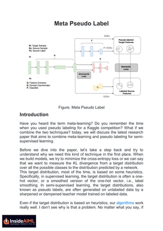
- 1. Meta Pseudo Label Figure. Meta Pseudo Label Introduction Have you heard the term meta-learning? Do you remember the time when you used pseudo labeling for a Kaggle competition? What if we combine the two techniques? today, we will discuss the latest research paper that aims to combine meta-learning and pseudo labeling for semi- supervised learning. Before we dive into the paper, let’s take a step back and try to understand why we need this kind of technique in the first place. When we build models, we try to minimize the cross-entropy loss or we can say that we want to measure the KL divergence from a target distribution over all the possible classes to the distribution predicted by a network. This target distribution, most of the time, is based on some heuristics. Specifically, in supervised learning, the target distribution is often a one- hot vector, or a smoothed version of the one-hot vector, i.e., label smoothing. In semi-supervised learning, the target distributions, also known as pseudo labels, are often generated on unlabeled data by a sharpened or dampened teacher model trained on labeled data. Even if the target distribution is based on heuristics, our algorithms work really well. I don’t see why is that a problem. No matter what you say, if
- 2. you are working with supervised learning or sem-supervised learning, you have to encode the target distribution in some way, right? Of course, the target distribution has to be constructed in some way. If one thing works well, then it doesn’t mean that it is the best way to do it. One of the drawbacks of these heuristics is that they cannot adapt to the learning state of the neural networks being trained. To this end, the authors propose to meta-learn the target distribution. They design a teacher model that assigns distributions to input examples to train the main model, the student model. Throughout the course of the student’s training, the teacher observes the student’s performance on a held-out validation set and learns to generate target distributions so that if the student learns from such distributions, the student will achieve good validation performance. Since the meta- learned target distributions play a similar role to pseudo labels, the authors named this method Meta Pseudo Label (MPL). Fine. I agree that these heuristics may not be the best ones. But the authors can’t just disprove it like this. There must be some motivation behind this proposal. Motivation For the sake of simplicity, the authors focused on training a C-way classification model parameterized by Θ, such as a neural network where we try to minimize the cross-entropy between a target distribution q∗(Y|X) and the model distribution pΘ(Y|X), i.e. Let’s see how the target distribution is defined in different conditions Supervised training: The target distribution is defined as the one-hot vector representing the ground-truth class, i.e., q∗(Y|x) = one-hot(y) Knowledge distillation: For each data point x, the predicted distribution of the large model q_large(x) is directly taken as the target distribution, i.e. q∗(Y|x) = q_large(Y|x) Semi-supervised learning: In SSL, a typical solution first employs an existing model qξ (trained on limited labeled data) to predict the class for each data point from an unlabeled set and utilizes the prediction to construct the target distribution which can be done in two ways: Hard label: q∗(Y|x) = one-hot (argmax (qξ(y|x)) Soft label: q∗(Y|x) = qξ(Y|x)
- 3. Also, MPL is not the first paper to talk about these non-optimal heuristics. Two very popular methods that try to mitigate this issue are: Label smoothing: It has been found that using one-hot vectors as the target distribution in a fully supervised machine translation and large- scale image classification such as ImageNet, can lead to overfitting. To combat this phenomenon, label smoothing proposes to smooth the one- hot distribution by allocating a small uniform weights to all classes. The target distribution is then redefined as: Temperature Tuning: For both knowledge distillation (KD) and soft- label SSL, it has been found that explicitly introducing a temperature hyper-parameter to modulate the target distribution could be very helpful. The logits l(x), are scaled by temperature τ. A value of τ < 1, sharpens the distribution and helps in speeding up the training. On the other hand, τ > 1, smoothens the distribution and helps to prevent over fitting. To this end, we can say that there are two intrinsic limitations of the current target distribution construction: However, instead of looking for better heuristics for designing the target distribution from scratch, we should look for a generic and systematic method that can be used to modify the target distribution in an existing algorithm that can lead to better performance. MPL tries to solve this. Meta Pseudo Labels Algorithm MPL tries to learn the target distribution q∗(x) throughout the course of training pΘ. The target distribution q∗(x) is parameterized as qΨ(x) where Ψ is trained using gradient descent. For the sake of simplicity, qΨ is taken as a classification model, which assigns the conditional probabilities to different classes of each input example x. (Medium is pretty bad when it comes to LaTex support � ) Here qΨ(x) serves the same role as q_large in knowledge distillation or qξ in SSL, as qΨ(x) provides the pseudo labels for pΘ to learn. Due to this similarity, the authors call qΨ the teacher model and pΘ the student model. As can be seen in the above figure, MPL update consists of two phases: Phase 1- The Student Learns from the Teacher: In this phase, given a single input example x, the teacher qΨ produces the conditional class
- 4. distribution qΨ(x) to train the student. The pair (x, qΨ(x)) is then shown to the student to update its parameters by backpropagating from the cross-entropy loss. For instance, if Θ is trained with SGD with a learning rate of η, then we have: Phase 2- The Teacher Learns from the Student’s Validation Loss: After the student updates its parameters as in Equation 1, its new parameter Θ(t+1) is evaluated on an example (xval, yval) from the held-out validation dataset, using the cross-entropy loss, L(yval, pΘ(t+1) (xval)). Since Θ(t+1) depends on Ψ via Equation 1, this validation cross-entropy loss is a function of Ψ. Specifically, dropping (xval, yval) from the equations for the sake of readability, we can write: Hold on a sec! The algorithm looks fine but I have a doubt. We are not using the original labels at all. It looks like that the pseudo labels generated by the teacher are enough to make corrections in both the models, right? Although the performance of the student model on the validation set allows the teacher model to adjust its parameter accordingly, the authors found out that this signal is not sufficient to train the teacher model. If we rely solely on the student signal, by the time the teacher model has seen enough evidence to generate meaningful target distribution, the student model might have started over fitting. A similar short-falling has been observed when training neural machine translation models with RL. To overcome this, the authors used supervised learning for the teacher. How? At each training step, apart from the MPL updates in Equation 2, the teacher also computes a gradient ∇Ψ(L(y, qΨ(x))) on a pair of labelled data (x, y). This gradient is then added to the MPL gradient ∇ΨR from Equation 2 to update the teacher’s parameters Ψ. Though this provides a sufficient signal to train the teacher, it poses another problem. We need to keep two classification models, the teacher, and the student, in memory. For smaller models, like ResNets, this won’t be a big problem but with larger models like EfficientNets, it limits the batch size leading to slow training time. To mitigate this issue, the authors designed a smaller alternative, ReducedMPL. A large model, q_large, is trained to convergence. Then, this model is used to pre-compute all target distributions for the student’s training data. Importantly, until this step, the student model has not been loaded into memory, effectively avoiding the large memory footprint of MPL. A
- 5. reduced teacher qΨ as a small and efficient network, such as a multi- layered perceptron, is parameterized to be trained along with the student. This reduced teacher qΨ takes as input the distribution predicted by the large teacher q_large and outputs a calibrated distribution for the student to learn. Experimental Results MPL is tested in two scenarios: Where limited data is available. Where the full labeled dataset is used. In both scenarios, experiments were performed on CIFAR-10, SVHN, and ImageNet. For experiments on full datasets, ReducedMPL was used due to the large memory footprint of MPL. ( I won’t be putting all the experimental details here. Please check the paper for the details.) Analysis MPL is not label correction: Since the teacher in MPL provides the target distribution for the student to learn and observes the student’s performance to improve itself, it is intuitive to think that the teacher tries to guess the correct labels for the student. To prove this, the authors plotted the training accuracy of all three: a purely supervised model, the teacher model, and the student model. The results look like this: As shown, the training accuracy of both the teacher and the student stays relatively low. Meanwhile, the training accuracy of the supervised model eventually reaches 100% much earlier. If MPL was simply performing label correction, then these accuracies should have been high. Instead, it looks like the teacher in MPL is trying to regularize the student to prevent overfitting which is crucial when you have a limited labeled dataset. MPL is Not Only a Regularization Strategy: As the authors said above that the teacher model in MPL is trying to regularize the student, it is easy to think that the teacher might be injecting noise so that the student doesn’t overfit. Turns out it isn’t the case. If the teacher has to inject noise in students’ training, it can do it in two ways: 1.) By flipping the
- 6. target class, eg. tell the student that the image of a car is an image of a horse. 2.)By dampening the target distribution. To confirm this, the authors visualized a few target distributions predicted by the teacher model in ReducedMPL for images in the TinyImages dataset. If you look at the above figure, you will notice that the label with the highest confidence for the images does not change at the quarters of the student’s training process. This means that the teacher has not managed to flip the target labels. Also, the target distributions that the teacher predicts become steeper between 50% and 75%. As the student is learning during this time, if the teacher simply wants to regularize the student, then the teacher should dampen the distributions. This observation is sufficient enough to prove that MPL isn’t just only a regularization method. Conclusion Overall the paper is well written. The ideas are crystal clear and thought- provoking. MPL makes use of both labeled and unlabeled data, making it a typical SSL algorithm but a significant difference between MPL and other SSL methods is that the teacher model receives learning signals from the student’s performance, and hence can adapt to the student’s learning state throughout the student’s training. To learn more about the Data Science algorithm visit the InsideAIML page.