Advanced Structural Dynamics - Eduardo Kausel

i
ADVANCED STRUCTURAL DYNAMICS
Advanced Structural Dynamics will appeal to a broad readership that includes
both undergraduate and graduate engineering students, doctoral candidates,
engineering scientists working in various technical disciplines, and practicing
professionals in an engineering office. The book has broad applicability and
draws examples from aeronautical, civil, earthquake, mechanical, and ocean
engineering, and at times it even dabbles in issues of geophysics and seismol-
ogy.The material presented is based on miscellaneous course and lecture notes
offered by the author at the Massachusetts Institute of Technology for many
years. The modular approach allows for a selective use of chapters, making it
appropriate for use not only as an introductory textbook but later on function-
ing also as a treatise for an advanced course, covering materials not typically
found in competing textbooks on the subject.
Professor Eduardo Kausel is a specialist in structural dynamics in the
Department of Civil Engineering at the Massachusetts Institute of Technology.
He is especially well known for two papers on the collapse of the Twin Towers
on September 11, 2001.The first of this pair, published on the web at MIT only
a few days after the terrorist act, attracted more readers around the world than
all other works and publications on the subject combined. Professor Kausel
is the author of the 2006 book Fundamental Solutions in Elastodynamics
(Cambridge University Press).

iii
Advanced Structural
Dynamics
EDUARDO KAUSEL
Massachusetts Institute of Technology

iv
University Printing House, Cambridge CB2 8BS, United Kingdom
One Liberty Plaza, 20th Floor, New York, NY 10006, USA
477 Williamstown Road, Port Melbourne,VIC 3207,Australia
4843/
24, 2nd Floor,Ansari Road, Daryaganj, Delhi – 110002, India
79 Anson Road, #06-
04/
06, Singapore 079906
Cambridge University Press is part of the University of Cambridge.
It furthers the University’s mission by disseminating knowledge in the pursuit of
education, learning, and research at the highest international levels of excellence.
www.cambridge.org
Information on this title: www.cambridge.org/
9781107171510
10.1017/9781316761403
© Eduardo Kausel 2017
This publication is in copyright. Subject to statutory exception
and to the provisions of relevant collective licensing agreements,
no reproduction of any part may take place without the written
permission of Cambridge University Press.
First published 2017
Printed in the United States of America by Sheridan Books, Inc.
A catalogue record for this publication is available from the British Library.
Library of Congress Cataloging-
in-
Publication Data
Names: Kausel, E.
Title:Advanced structural dynamics / by Eduardo Kausel, Massachusetts Institute of Technology.
Other titles: Structural dynamics
Description: Cambridge [England]: Cambridge University Press, 2017
. |
Includes bibliographical references and index.
Identifiers: LCCN 2016028355 | ISBN 9781107171510 (hard back)
Subjects: LCSH: Structural dynamics – Textbooks. | Structural analysis (Engineering) – Textbooks.
Classification: LCC TA654.K276 2016 | DDC 624.1/71–dc23
LC record available at https://lccn.loc.gov/2016028355
ISBN 978-1-107-17151-0 Hardback
Cambridge University Press has no responsibility for the persistence or accuracy of URLs
for external or third-
party Internet Web sites referred to in this publication and does not
guarantee that any content on such Web sites is, or will remain, accurate or appropriate.

v
To my former graduate student and dear Guardian Angel Hyangly Lee,
in everlasting gratitude for her continued support of my work at MIT.

vii
vii
Contents
Preface page xxi
Notation and Symbols xxv
Unit Conversions xxix
1 Fundamental Principles 1
1.1 Classification of Problems in Structural Dynamics 1
1.2 Stress–Strain Relationships 2
1.2.1 Three-
Dimensional State of Stress–
Strain 2
1.2.2 Plane Strain 2
1.2.3 Plane Stress 2
1.2.4 Plane Stress versus Plane Strain: Equivalent
Poisson’s Ratio 3
1.3 Stiffnesses of Some Typical Linear Systems 3
1.4 Rigid Body Condition of Stiffness Matrix 11
1.5 Mass Properties of Rigid, Homogeneous Bodies 12
1.6 Estimation of Miscellaneous Masses 17
1.6.1 Estimating the Weight (or Mass) of a Building 17
1.6.2 Added Mass of Fluid for Fully Submerged
Tubular Sections 18
1.6.3 Added Fluid Mass and Damping for Bodies Floating
in Deep Water 20
1.7 Degrees of Freedom 20
1.7
.1 Static Degrees of Freedom 20
1.7
.2 Dynamic Degrees of Freedom 21
1.8 Modeling Structural Systems 22
1.8.1 Levels of Abstraction 22
1.8.2 Transforming Continuous Systems into Discrete Ones 25
Heuristic Method 25
1.8.3 Direct Superposition Method 26
1.8.4 Direct Stiffness Approach 26
1.8.5 Flexibility Approach 27
1.8.6 Viscous Damping Matrix 29

Contents
viii
viii
1.9 Fundamental Dynamic Principles for a Rigid Body 31
1.9.1 Inertial Reference Frames 31
1.9.2 Kinematics of Motion 31
Cardanian Rotation 32
Eulerian Rotation 33
1.9.3 Rotational Inertia Forces 34
1.9.4 Newton’s Laws 35
(a) Rectilinear Motion 35
(b) Rotational Motion 36
1.9.5 Kinetic Energy 36
1.9.6 Conservation of Linear and Angular Momentum 36
(a) Rectilinear Motion 37
(b) Rotational Motion 37
1.9.7 D’
Alembert’s Principle 37
1.9.8 Extension of Principles to System of Particles and
Deformable Bodies 38
1.9.9 Conservation of Momentum versus
Conservation of Energy 38
1.9.10 Instability of Rigid Body Spinning Freely in Space 39
1.10 Elements of Analytical Mechanics 39
1.10.1 Generalized Coordinates and Its Derivatives 40
1.10.2 Lagrange’s Equations 42
(a) Elastic Forces 42
(b) Damping Forces 43
(c) External Loads 44
(d) Inertia Forces 45
(e) Combined Virtual Work 45
2 Single Degree of Freedom Systems 55
2.1 The Damped SDOF Oscillator 55
2.1.1 Free Vibration: Homogeneous Solution 56
Underdamped Case (ξ < 1) 57
Critically Damped Case (ξ = 1) 58
Overdamped Case (ξ > 1) 59
2.1.2 Response Parameters 59
2.1.3 Homogeneous Solution via Complex Frequencies:
System Poles 60
2.1.4 Free Vibration of an SDOF System with
Time-Varying Mass 61
2.1.5 Free Vibration of SDOF System with
Frictional Damping 63
(a) System Subjected to Initial Displacement 64
(b) Arbitrary Initial Conditions 65
2.2 Phase Portrait: Another Way to View Systems 67
2.2.1 Preliminaries 67
2.2.2 Fundamental Properties of Phase Lines 69
Trajectory Arrows 69
Intersection of Phase Lines with Horizontal Axis 70
Asymptotic Behavior at Singular Points and Separatrix 70
Period of Oscillation 71

Contents ix
ix
2.2.3 Examples of Application 71
Phase Lines of a Linear SDOF System 71
Ball Rolling on a Smooth Slope 71
2.3 Measures of Damping 73
2.3.1 Logarithmic Decrement 74
2.3.2 Number of Cycles to 50% Amplitude 75
2.3.3 Other Forms of Damping 76
2.4 Forced Vibrations 76
2.4.1 Forced Vibrations: Particular Solution 76
(a) Heuristic Method 77
(b) Variation of Parameters Method 78
2.4.2 Forced Vibrations: General Solution 79
2.4.3 Step Load of Infinite Duration 80
2.4.4 Step Load of Finite Duration (Rectangular Load,
or Box Load) 81
2.4.5 Impulse Response Function 81
2.4.6 Arbitrary Forcing Function: Convolution 83
Convolution Integral 83
Time Derivatives of the Convolution Integral 84
Convolution as a Particular Solution 84
2.5 Support Motion in SDOF Systems 85
2.5.1 General Considerations 85
2.5.2 Response Spectrum 88
Tripartite Spectrum 88
2.5.3 Ship on Rough Seas, or Car on Bumpy Road 89
2.6 Harmonic Excitation: Steady-
State Response 92
2.6.1 Transfer Function Due to Harmonic Force 92
2.6.2 Transfer Function Due to Harmonic Support Motion 96
2.6.3 Eccentric Mass Vibrator 100
Experimental Observation 101
2.6.4 Response to Suddenly Applied Sinusoidal Load 102
2.6.5 Half-
Power Bandwidth Method 103
Application of Half-
Power Bandwidth Method 105
2.7 Response to Periodic Loading 106
2.7
.1 Periodic Load Cast in Terms of Fourier Series 106
2.7
.2 Nonperiodic Load as Limit of Load with
Infinite Period 107
2.7
.3 System Subjected to Periodic Loading: Solution in the
Time Domain 109
2.7
.4 Transfer Function versus Impulse Response Function 111
2.7
.5 Fourier Inversion of Transfer Function by Contour
Integration 111
Location of Poles, Fourier Transforms, and Causality 113
2.7
.6 Response Computation in the Frequency Domain 114
(1) Trailing Zeros 115
(2) Exponential Window Method: The
Preferred Strategy 115
2.8 Dynamic Stiffness or Impedance 115
2.8.1 Connection of Impedances in Series and/
or Parallel 117
Standard Solid 118

Contents
x
x
2.9 Energy Dissipation through Damping 118
2.9.1 Viscous Damping 119
Instantaneous Power and Power Dissipation 119
Human Power 120
Average Power Dissipated in Harmonic Support
Motion 120
Ratio of Energy Dissipated to Energy Stored 121
Hysteresis Loop for Spring–Dashpot System 122
2.9.2 Hysteretic Damping 123
Ratio of Energy Dissipated to Energy Stored 123
Instantaneous Power and Power Dissipation via the
Hilbert Transform 124
2.9.3 Power Dissipation during Broadband Base Excitation 124
2.9.4 Comparing the Transfer Functions for
Viscous and Hysteretic Damping 125
Best Match between Viscous and Hysteretic Oscillator 126
2.9.5 Locus of Viscous and Hysteretic Transfer Function 127
3 Multiple Degree of Freedom Systems 131
3.1 Multidegree of Freedom Systems 131
3.1.1 Free Vibration Modes of Undamped MDOF Systems 131
Orthogonality Conditions 132
Normalized Eigenvectors 134
3.1.2 Expansion Theorem 134
3.1.3 Free Vibration of Undamped System Subjected
to Initial Conditions 137
3.1.4 Modal Partition of Energy in an Undamped
MDOF System 137
3.1.5 What If the Stiffness and Mass Matrices Are
Not Symmetric? 138
3.1.6 Physically Homogeneous Variables and Dimensionless
Coordinates 139
3.2 Effect of Static Loads on Structural Frequencies: Π-
Δ Effects 141
3.2.1 Effective Lateral Stiffness 141
3.2.2 Vibration of Cantilever Column under Gravity Loads 144
3.2.3 Buckling of Column with Rotations Prevented 145
3.2.4 Vibration of Cantilever Shear Beam 146
3.3 Estimation of Frequencies 146
3.3.1 Rayleigh Quotient 147
Rayleigh–Schwarz Quotients 149
3.3.2 Dunkerley–Mikhlin Method 149
Dunkerley’s Method for Systems with
Rigid-Body Modes 154
3.3.3 Effect on Frequencies of a Perturbation in the
Structural Properties 157
Perturbation of Mass Matrix 158
Perturbation of Stiffness Matrix 159
Qualitative Implications of Perturbation Formulas 160

Contents xi
xi
3.4 Spacing Properties of Natural Frequencies 162
3.4.1 The Minimax Property of Rayleigh’s Quotient 162
3.4.2 Interlacing of Eigenvalues for Systems with Single
External Constraint 165
Single Elastic External Support 166
3.4.3 Interlacing of Eigenvalues for Systems with Single
Internal Constraint 167
Single Elastic Internal Constraint 167
3.4.4 Number of Eigenvalues in Some Frequency Interval 167
Sturm Sequence Property 167
The Sign Count of the Shifted Stiffness Matrix 168
Root Count for Dynamically Condensed Systems 170
Generalization to Continuous Systems 173
3.5 Vibrations of Damped MDOF Systems 176
3.5.1 Vibrations of Proportionally Damped MDOF Systems 176
3.5.2 Proportional versus Nonproportional Damping Matrices 181
3.5.3 Conditions under Which a Damping Matrix Is
Proportional 181
3.5.4 Bounds to Coupling Terms in Modal Transformation 183
3.5.5 Rayleigh Damping 184
3.5.6 Caughey Damping 185
3.5.7 Damping Matrix Satisfying Prescribed Modal
Damping Ratios 189
3.5.8 Construction of Nonproportional Damping Matrices 191
3.5.9 Weighted Modal Damping: The Biggs–
Roësset
Equation 194
3.6 Support Motions in MDOF Systems 196
3.6.1 Structure with Single Translational DOF at Each
Mass Point 197
Solution by Modal Superposition (Proportional
Damping) 198
3.6.2 MDOF System Subjected to Multicomponent
Support Motion 200
3.6.3 Number of Modes in Modal Summation 203
3.6.4 Static Correction 205
3.6.5 Structures Subjected to Spatially Varying
Support Motion 207
3.7 Nonclassical, Complex Modes 209
3.7
.1 Quadratic Eigenvalue Problem 210
3.7
.2 Poles or Complex Frequencies 210
3.7
.3 Doubled-Up Form of Differential Equation 213
3.7
.4 Orthogonality Conditions 215
3.7
.5 Modal Superposition with Complex Modes 216
3.7
.6 Computation of Complex Modes 221
3.8 Frequency Domain Analysis of MDOF Systems 223
3.8.1 Steady-
State Response of MDOF Systems to
Structural Loads 223
3.8.2 Steady-
State Response of MDOF System Due to
Support Motion 224

Contents
xii
xii
3.8.3 In-
Phase,Antiphase, and Opposite-
Phase Motions 231
3.8.4 Zeros of Transfer Functions at Point of
Application of Load 233
3.8.5 Steady-
State Response of Structures with
Hysteretic Damping 234
3.8.6 Transient Response of MDOF Systems via
Fourier Synthesis 235
3.8.7 Decibel Scale 236
3.8.8 Reciprocity Principle 236
3.9 Harmonic Vibrations Due to Vortex Shedding 238
3.10 Vibration Absorbers 239
3.10.1 Tuned Mass Damper 239
3.10.2 Lanchester Mass Damper 243
3.10.3 Examples of Application of Vibration Absorbers 244
3.10.4 Torsional Vibration Absorber 249
4 Continuous Systems 251
4.1 Mathematical Characteristics of Continuous Systems 251
4.1.1 Taut String 251
4.1.2 Rods and Bars 252
4.1.3 Bending Beam, Rotational Inertia Neglected 252
4.1.4 Bending Beam, Rotational Inertia Included 254
4.1.5 Timoshenko Beam 254
4.1.6 Plate Bending 256
4.1.7 Vibrations in Solids 257
4.1.8 General Mathematical Form of Continuous Systems 258
4.1.9 Orthogonality of Modes in Continuous Systems 259
4.2 Exact Solutions for Simple Continuous Systems 260
4.2.1 Homogeneous Rod 260
Normal Modes of a Finite Rod 262
Fixed–Fixed Rod 262
Free–Free Rod 263
Fixed–Free Rod 264
Normal Modes of a Rod without Solving a
Differential Equation 264
Orthogonality of Rod Modes 265
4.2.2 Euler–
Bernoulli Beam (Bending Beam) 267
Normal Modes of a Finite-
Length Euler–
Bernoulli
Beam 268
Simply Supported Beam 269
Other Boundary Conditions 269
Normal Modes of a Free–
Free Beam 270
Normal Modes of a Cantilever Beam 273
Orthogonality Conditions of a Bending Beam 274
Strain and Kinetic Energies of a Beam 274
4.2.3 Bending Beam Subjected to Moving Harmonic Load 274
Homogeneous Solution 275
Particular Solution 275
4.2.4 Nonuniform Bending Beam 277

Contents xiii
xiii
4.2.5 Nonclassical Modes of Uniform Shear Beam 279
Dynamic Equations of Shear Beam 280
Modes of Rotationally Unrestrained Shear Beam 281
Concluding Observations 287
4.2.6 Inhomogeneous Shear Beam 287
Solution for Shear Modulus Growing Unboundedly
with Depth 288
Finite Layer of Inhomogeneous Soil 289
Special Case: Shear Modulus Zero at Free Surface 290
Special Case: Linearly Increasing Shear
Wave Velocity 291
4.2.7 Rectangular Prism Subjected to SH Waves 292
Normal Modes 292
Forced Vibration 293
4.2.8 Cones, Frustums, and Horns 295
(a) Exponential Horn 296
(b)
Frustum Growing as a Power of the Axial
Distance 299
(c)
Cones of Infinite Depth with Bounded Growth
of Cross Section 301
4.2.9 Simply Supported, Homogeneous, Rectangular Plate 302
Orthogonality Conditions of General Plate 302
Simply Supported, Homogeneous Rectangular Plate 303
4.3 Continuous,Wave-
Based Elements (Spectral Elements) 305
4.3.1 Impedance of a Finite Rod 306
4.3.2 Impedance of a Semi-
infinite Rod 311
4.3.3 Viscoelastic Rod on a Viscous Foundation
(Damped Rod) 311
Stress and Velocity 313
Power Flow 314
4.3.4 Impedance of a Euler Beam 318
4.3.5 Impedance of a Semi-
infinite Beam 322
4.3.6 Infinite Euler Beam with Springs at Regular Intervals 323
Cutoff Frequencies 326
Static Roots 327
4.3.7 Semi-
infinite Euler Beam Subjected
to Bending Combined with Tension 328
Power Transmission 331
Power Transmission after Evanescent Wave
Has Decayed 331
5 Wave Propagation 333
5.1 Fundamentals of Wave Propagation 333
5.1.1 Waves in Elastic Bodies 333
5.1.2 Normal Modes and Dispersive Properties of
Simple Systems 334
An Infinite Rod 334
Gravity Waves in a Deep Ocean 336
An Infinite Bending Beam 337

Contents
xiv
xiv
A Bending Beam on an Elastic Foundation 338
A Bending Beam on an Elastic Half-
Space 340
Elastic Thick Plate (Mindlin Plate) 341
5.1.3 Standing Waves,Wave Groups, Group Velocity, and
Wave Dispersion 342
Standing Waves 342
Groups and Group Velocity 343
Wave Groups and the Beating Phenomenon 344
Summary of Concepts 344
5.1.4 Impedance of an Infinite Rod 345
5.2 Waves in Layered Media via Spectral Elements 348
5.2.1 SH Waves and Generalized Love Waves 349
(A) Normal Modes 353
(B) Source Problem 355
(C) Wave Amplification Problem 355
5.2.2 SV-
P Waves and Generalized Rayleigh Waves 358
Normal Modes 362
5.2.3 Stiffness Matrix Method in Cylindrical Coordinates 362
5.2.4 Accurate Integration of Wavenumber Integrals 365
Maximum Wavenumber for Truncation and
Layer Coupling 366
Static Asymptotic Behavior: Tail of Integrals 367
Wavenumber Step 369
6 Numerical Methods 371
6.1 Normal Modes by Inverse Iteration 371
6.1.1 Fundamental Mode 371
6.1.2 Higher Modes: Gram–
Schmidt Sweeping Technique 374
6.1.3 Inverse Iteration with Shift by Rayleigh Quotient 374
6.1.4 Improving Eigenvectors after Inverse Iteration 376
6.1.5 Inverse Iteration for Continuous Systems 377
6.2 Method of Weighted Residuals 378
6.2.1 Point Collocation 381
6.2.2 Sub-domain 381
6.2.3 Least Squares 381
6.2.4 Galerkin 381
6.3 Rayleigh–Ritz Method 384
6.3.1 Boundary Conditions and Continuity Requirements
in Rayleigh–Ritz 385
6.3.2 Rayleigh–
Ritz versus Galerkin 386
6.3.3 Rayleigh–
Ritz versus Finite Elements 387
6.3.4 Rayleigh–
Ritz Method for Discrete Systems 388
6.3.5 Trial Functions versus True Modes 390
6.4 Discrete Systems via Lagrange’s Equations 391
6.4.1 Assumed Modes Method 391
6.4.2 Partial Derivatives 391
6.4.3 Examples of Application 392
6.4.4 What If Some of the Discrete Equations Remain
Uncoupled? 399

Contents xv
xv
6.5 Numerical Integration in the Time Domain 400
6.5.1 Physical Approximations to the Forcing Function 401
6.5.2 Physical Approximations to the Response 403
Constant Acceleration Method 403
Linear Acceleration Method 404
Newmark’s β Method 404
Impulse Acceleration Method 405
6.5.3 Methods Based on Mathematical Approximations 406
Multistep Methods for First-
Order Differential
Equations 407
Difference and Integration Formulas 409
Multistep Methods for Second-
Order Differential
Equations 409
6.5.4 Runge–Kutta Type Methods 410
Euler’s Method 411
Improved and Modified Euler Methods 411
The Normal Runge–
Kutta Method 412
6.5.5 Stability and Convergence Conditions for Multistep
Methods 413
Conditional and Unconditional Stability of Linear
Systems 413
6.5.6 Stability Considerations for Implicit Integration
Schemes 416
6.6 Fundamentals of Fourier Methods 417
6.6.1 Fourier Transform 417
6.6.2 Fourier Series 420
6.6.3 Discrete Fourier Transform 422
6.6.4 Discrete Fourier Series 423
6.6.5 The Fast Fourier Transform 426
6.6.6 Orthogonality Properties of Fourier Expansions 427
(a) Fourier Transform 427
(b) Fourier Series 427
(c) Discrete Fourier Series 427
6.6.7 Fourier Series Representation of a Train of Periodic
Impulses 428
6.6.8 Wraparound, Folding, and Aliasing 428
6.6.9 Trigonometric Interpolation and the Fundamental
Sampling Theorem 430
6.6.10 Smoothing, Filtering,Truncation, and
Data Decimation 432
6.6.11 Mean Value 432
6.6.12 Parseval’s Theorem 433
6.6.13 Summary of Important Points 434
6.6.14 Frequency Domain Analysis of Lightly
Damped or Undamped Systems 434
Exponential Window Method: The Preferred Tool 435
6.7 Fundamentals of Finite Elements 440
6.7
.1 Gaussian Quadrature 441
Normalization 442

Contents
xvi
xvi
6.7
.2 Integration in the Plane 444
(a) Integral over a Rectangular Area 446
(b) Integral over a Triangular Area 447
(c) Curvilinear Triangle 448
(d) Quadrilateral 450
(e) Curvilinear Quadrilateral 451
Inadmissible Shapes 451
6.7
.3 Finite Elements via Principle of Virtual Displacements 451
(a) Consistency 454
(b) Conformity 454
(c) Rigid Body Test 454
(d) Convergence (Patch Test) 454
6.7
.4 Plate Stretching Elements (Plane Strain) 455
(a) Triangular Element 455
(b) Rectangular Element 457
6.7
.5 Isoparametric Elements 459
Plane Strain Curvilinear Quadrilaterals 459
Cylindrical Coordinates 463
7 Earthquake Engineering and Soil Dynamics 481
7
.1 Stochastic Processes in Soil Dynamics 481
7
.1.1 Expectations of a Random Process 481
7
.1.2 Functions of Random Variable 482
7
.1.3 Stationary Processes 482
7
.1.4 Ergodic Processes 483
7
.1.5 Spectral Density Functions 483
7
.1.6 Coherence Function 484
7
.1.7 Estimation of Spectral Properties 484
7
.1.8 Spatial Coherence of Seismic Motions 488
Coherency Function Based on Statistical
Analyses of Actual Earthquake Motions 488
Wave Model for Random Field 490
Simple Cross-
Spectrum for SH Waves 490
Stochastic Deconvolution 493
7
.2 Earthquakes, and Measures of Quake Strength 494
7
.2.1 Magnitude 495
Seismic Moment 495
Moment Magnitude 497
7
.2.2 Seismic Intensity 497
7
.2.3 Seismic Risk: Gutenberg–Richter Law 499
7
.2.4 Direction of Intense Shaking 500
7
.3 Ground Response Spectra 502
7
.3.1 Preliminary Concepts 502
7
.3.2 Tripartite Response Spectrum 504
7
.3.3 Design Spectra 505
7
.3.4 Design Spectrum in the style of ASCE/
SEI-
7-
05 506
Design Earthquake 506

Contents xvii
x
v
i
i
Transition Periods 506
Implied Ground Motion Parameters 507
7
.3.5 MDOF Systems: Estimating Maximum Values from
Response Spectra 507
Common Error in Modal Combination 510
General Case: Response Spectrum Estimation for
Complete Seismic Environment 511
7
.4 Dynamic Soil–
Structure Interaction 513
7
.4.1 General Considerations 513
Seismic Excitation (Free-
Field Problem) 514
Kinematic Interaction 514
Inertial Interaction 515
7
.4.2 Modeling Considerations 515
Continuum Solutions versus Finite Elements 515
Finite Element Discretization 515
Boundary Conditions 516
7
.4.3 Solution Methods 517
Direct Approach 517
Superposition Theorem 518
Three-Step Approach 519
Approximate Stiffness Functions 520
7
.4.4 Direct Formulation of SSI Problems 522
The Substructure Theorem 522
SSI Equations for Structures with Rigid Foundation 524
7
.4.5 SSI via Modal Synthesis in the Frequency Domain 526
Partial Modal Summation 529
What If the Modes Occupy Only a Subspace? 531
Member Forces 533
7
.4.6 The Free-Field Problem: Elements of 1-
D Soil
Amplification 534
Effect of Location of Control Motion in 1-
D Soil
Amplification 537
7
.4.7 Kinematic Interaction of Rigid Foundations 540
Iguchi’s Approximation, General Case 541
Iguchi Approximation for Cylindrical Foundations
Subjected to SH Waves 544
Geometric Properties 545
Free-
Field Motion Components at Arbitrary Point,
Zero Azimuth 546
Surface Integrals 546
Volume Integrals 548
Effective Motions 549
7
.5 Simple Models for Time-
Varying, Inelastic Soil Behavior 551
7
.5.1 Inelastic Material Subjected to Cyclic Loads 551
7
.5.2 Masing’s Rule 553
7
.5.3 Ivan’s Model: Set of Elastoplastic Springs in Parallel 555
7
.5.4 Hyperbolic Model 556
7
.5.5 Ramberg–Osgood Model 558

Contents
xviii
x
v
i
i
i
7
.6 Response of Soil Deposits to Blast Loads 561
7
.6.1 Effects of Ground-
Borne Blast Vibrations on
Structures 561
Frequency Effects 561
Distance Effects 562
Structural Damage 563
8 Advanced Topics 565
8.1 The Hilbert Transform 565
8.1.1 Definition 565
8.1.2 Fourier Transform of the Sign Function 566
8.1.3 Properties of the Hilbert Transform 567
8.1.4 Causal Functions 569
8.1.5 Kramers–
Kronig Dispersion Relations 570
Minimum Phase Systems 572
Time-Shifted Causality 573
8.2 Transfer Functions, Normal Modes, and Residues 573
8.2.1 Poles and Zeros 573
8.2.2 Special Case: No Damping 574
8.2.3 Amplitude and Phase of the Transfer Function 575
8.2.4 Normal Modes versus Residues 577
8.3 Correspondence Principle 580
8.4 Numerical Correspondence of Damped and
Undamped Solutions 582
8.4.1 Numerical Quadrature Method 582
8.4.2 Perturbation Method 584
8.5 Gyroscopic Forces Due to Rotor Support Motions 585
8.6 Rotationally Periodic Structures 590
8.6.1 Structures Composed of Identical Units and with
Polar Symmetry 590
8.6.2 Basic Properties of Block-
Circulant Matrices 593
8.6.3 Dynamics of Rotationally Periodic Structures 594
8.7 Spatially Periodic Structures 596
8.7
.1 Method 1: Solution in Terms of Transfer Matrices 596
8.7
.2 Method 2: Solution via Static Condensation and
Cloning 602
Example: Waves in a Thick Solid Rod Subjected
to Dynamic Source 603
8.7
.3 Method 3: Solution via Wave Propagation Modes 604
Example 1: Set of Identical Masses Hanging
from a Taut String 605
Example 2: Infinite Chain of Viscoelastically
Supported Masses and Spring-
Dashpots 608
8.8 The Discrete Shear Beam 610
8.8.1 Continuous Shear Beam 611
8.8.2 Discrete Shear Beam 611

Contents xix
xix
9 Mathematical Tools 619
9.1 Dirac Delta and Related Singularity Functions 619
9.1.1 Related Singularity Functions 620
Doublet Function 620
Dirac Delta Function 620
Unit Step Function (Heaviside Function) 620
Unit Ramp Function 621
9.2 Functions of Complex Variables: A Brief Summary 621
9.3 Wavelets 626
9.3.1 Box Function 626
9.3.2 Hanning Bell (or Window) 626
9.3.3 Gaussian Bell 627
9.3.4 Modulated Sine Pulse (Antisymmetric Bell) 628
9.3.5 Ricker Wavelet 628
9.4 Useful Integrals Involving Exponentials 630
9.4.1 Special Cases 630
9.5 Integration Theorems in Two and Three Dimensions 630
9.5.1 Integration by Parts 631
9.5.2 Integration Theorems 631
9.5.3 Particular Cases: Gauss, Stokes, and Green 633
9.6 Positive Definiteness of Arbitrary Square Matrix 633
9.7 Derivative of Matrix Determinant: The Trace Theorem 640
9.8 Circulant and Block-
Circulant Matrices 642
9.8.1 Circulant Matrices 642
9.8.2 Block-Circulant Matrices 644
10 Problem Sets 647
Author Index 713
Subject Index 714

xxi
xxi
Preface
The material in this book slowly accumulated,accreted,and grew out of the many lectures
on structural dynamics, soil dynamics, earthquake engineering, and structural mechanics
that I gave at MIT in the course of several decades of teaching. At first these constituted
mere handouts to the students, meant to clarify further the material covered in the lec-
tures,but soon the notes transcended the class environment and began steadily growing in
size and content as well as complication. Eventually, the size was such that I decided that
it might be worthwhile for these voluminous class notes to see the light as a regular text-
book, but the sheer effort required to clean out and polish the text so as to bring it up to
publication standards demanded too much of my time and entailed sacrifices elsewhere
in my busy schedule that I simply couldn’t afford. Or expressing it in MIT-
speak, I applied
the Principle of Selective Neglect. But after years (and even decades) of procrastination,
eventually I finally managed to break the vicious cycle of writer’s block and brought this
necessary task to completion.
Make no mistake: the material covered in this book far exceeds what can be taught in
any one-
semester graduate course in structural dynamics or mechanical vibration, and
indeed, even in a sequence of two such courses. Still, it exhaustively covers the funda-
mentals in vibration theory, and then goes on well beyond the standard fare in –and
conventional treatment of –a graduate course in structural dynamics, as a result of which
most can (and should) be excluded from an introductory course outline, even if it can still
be used for that purpose. Given the sheer volume of material, the text is admittedly terse
and at times rather sparse in explanations, but that is deliberate, for otherwise the book
would have been unduly long, not to mention tedious to read and follow.Thus, the reader
is expected to have some background in the mechanical sciences such that he or she need
not be taken by the hand. Still, when used in the classroom for a first graduate course, it
would suffice to jump over advanced sections, and do so without sacrifices in the clarity
and self-
sufficiency of the retained material.
In a typical semester, I would start by reviewing the basic principles of dynam-
ics, namely Newton’s laws, impulse and conservation of linear and angular momenta,
D’
Alembert’s principle, the concept of point masses obtained by means of mass lumping
and tributary areas, and most importantly, explicating the difference between static and
dynamic degrees of freedom (or master–
slave DOF), all while assuming small displace-
ments and skipping initially over the section that deals with Lagrange’s equations. From

Preface
xxii
x
x
i
i
there on I would move on to cover the theory of single-
DOF systems and devote just
about half of the semester to that topic, inasmuch as multi-
DOF systems and continu-
ous systems can largely be regarded as generalizations of those more simple systems. In
the lectures, I often interspersed demonstration experiments to illustrate basic concepts
and made use of brief Matlab®
models to demonstrate the application of the concepts
being learned. I also devoted a good number of lectures to explain harmonic analysis
and the use of complex Fourier series, which in my view is one of the most important
yet difficult concepts for students to comprehend and assimilate properly. For that pur-
pose, I usually started by explaining the concepts of amplitude and phase by consider-
ing a simple complex number of the form z x y
= + i , and then moving on to see what
those quantities would be for products and ratios of complex numbers of the form z z z
= 1 2,
z z z z z
= = −
( )
1 2 1 2
1 2
/ / ei φ φ
, and in particular z z z
= = −
1 2 2
2
/ /
e iφ
. I completely omitted the use
of sine and cosine Fourier series, and considered solely the complex exponential form of
Fourier series and the Fourier transform, which I used in the context of periodic loads,
and then in the limit of an infinite period, namely a transient load. From there the rela-
tionship between impulse response function and transfer functions arose naturally. In
the context of harmonic analysis, I would also demonstrate the great effectiveness of the
(virtually unknown) Exponential Window Method (in essence, a numerical implementa-
tion of the Laplace Transform) for the solution of lightly damped system via complex
frequencies, which simultaneously disposes of the problems of added trailing zeroes and
undesired periodicity of the response function, and thus ultimately of the “wraparound”
problem, that is, causality.
Discrete systems would then take me some two thirds of the second half of the semes-
ter, focusing on classical modal analysis and harmonic analysis, and concluding with some
lectures on the vibration absorber. This left me just about one third of the half semester
(i.e., some two to three weeks) for the treatment of continuous systems, at which time
I would introduce the use of Lagrange’s equations as a tool to solve continuous media by
discretizing those systems via the Assumed Modes Method.
In the early version of the class lecture notes I included support motions and ground
response spectra as part of the single-
DOF lectures. However, as the material dealing
with earthquake engineering grew in size and extent, in due time I moved that material
out to a separate section, even if I continued to make seamless use of parts of those in my
classes.
Beyond lecture materials for the classroom, this book contains extensive materials not
included in competing books on structural dynamics, of which there already exist a pleth-
ora of excellent choices, and this was the main reason why I decided it was worthwhile
to publish it. For this reason, I also expect this book to serve as a valuable reference for
practicing engineers, and perhaps just as importantly, to aspiring young PhD graduates
with academic aspirations in the fields of structural dynamics, soil dynamics, earthquake
engineering, or mechanical vibration.
Last but not least, I wish to acknowledge my significant indebtedness and gratitude
to Prof. José Manuel Roësset, now retired from the Texas AM University, for his
most invaluable advice and wisdom over all of the years that have spanned my aca-
demic career at MIT. It was while I was a student and José a tenured professor here
that I learned with him mechanics and dynamics beyond my wildest expectations and

Preface xxiii
x
x
i
i
i
dreams, and it could well be said that everything I know and acquired expertise in is
ultimately due to him, and that in a very real sense he has been the ghost writer and
coauthor of this book.
In problems relating to vibrations, nature has provided us with a range of mysteries which
for their elucidation require the exercise of a certain amount of mathematical dexterity. In
many directions of engineering practice, that vague commodity known as common sense
will carry one a long way, but no ordinary mortal is endowed with an inborn instinct for
vibrations; mechanical vibrations in general are too rapid for the utilization of our sense
of sight, and common sense applied to these phenomena is too common to be other than
a source of danger.
C. E. Inglis, FRS, James Forrest Lecture, 1944

x
x
v
xxv
Notation and Symbols
Although we may from time to time change the meaning of certain symbols and deviate
temporarily from the definitions given in this list, by and large we shall adopt in this book
the notation given herein, and we shall do so always in the context of an upright, right-
handed coordinate system.
Vectors and matrices: we use boldface symbols, while non-
boldface symbols (in italics)
are scalars.Capital letters denote matrices,and lowercase letters are vectors.(Equivalence
with blackboard symbols: q
~
is the same as q, and M is the same as M).
Special Constants (non-
italic)
e Natural base of logarithms = 2.71828182845905…
i Imaginary unit = −1
π 3.14159265358979…
Roman Symbols
a Acceleration
a Acceleration vector
A Amplitude of a transfer function or a wave; also area or cross section
As Shear area
b Body load, b b t
= ( )
x,
b Vector of body loads, b b x
= ( )
,t
c Viscous damping (dashpot) constant
C C
1 2
, Constants of integration
CS Shear wave velocity G/ρ
( )
Cr Rod wave velocity E/ρ
( )
Cf Flexural wave velocity C R
r ω
( )
C Viscous damping matrix
 Modally transformed, diagonal damping matrix (Φ Φ
T
C )
D Diameter
f Frequency in Hz; it may also denote a flexibility

xxvi
x
x
v
i
fd Damped natural frequency, in Hz
fn Natural frequency, in Hz
ê Cartesian, unit base vector ˆ , ˆ , ˆ ˆ,ˆ, ˆ
e e e i j k
1 2 3 ≡
( )
E Young’s modulus, E G
= +
( )
2 1 ν
Ed Energy dissipated
Es Elastic energy stored
ĝ Curvilinear base vector ˆ , ˆ , ˆ
g g g
1 2 3
( )
g Acceleration of gravity
g t
( ) Unit step-
load response function
G Shear modulus
h Depth or thickness of beam, element, or plate
h t
( ) Impulse response function
H Height
H ω
( ) Transfer function (frequency response function for a unit input)
I Area moment of inertia
j Most often an index for a generic mode
J Mass moment of inertia
k Usually stiffness, but sometimes a wavenumber
kc Complex stiffness or impedance
K Kinetic energy
K Stiffness matrix
L Length of string, rod, beam, member, or element
m Mass
M Mass matrix
n Abbreviation for natural; also, generic degree of freedom
N Total number of degrees of freedom
p t
( ) Applied external force

p ω
( ) Fourier transform of p t
( ), i.e., load in the frequency domain
p0 Force magnitude
p External force vector, p p
= ( )
t
q t
( ) Generalized coordinate, or modal coordinate
q t
( ) Vector of generalized coordinates
r Tuning ratio r n
= ω ω
/ ; radial coordinate
r Radial position vector
R Radius of gyration or geometric radius
Sa Ground response spectrum for absolute acceleration (pseudo-
acceleration)
Sd Ground response spectrum for relative displacements
Sv Ground response spectrum for relative pseudo-velocity
t Time
td Time duration of load
tp Period of repetition of load
T Period (= 1/f ), or duration
Td Damped natural period

Notation and Symbols xxvii
x
x
v
i
i
Tn Natural period
u t
( ) Absolute displacement. In general, u u t u x y z t
= ( ) = ( )
x, , , ,

u ω
( ) Fourier transform of u t
( ); frequency response function
u0 Initial displacement, or maximum displacement

u0 Initial velocity
ug Ground displacement
uh Homogeneous solution (free vibration)
up Particular solution
up0 Initial displacement value (not condition!) of particular solution

up0 Initial velocity value (not condition!) of particular solution
u Absolute displacement vector

u Absolute velocity vector

u Absolute acceleration vector
v Relative displacement (scalar)
v Relative displacement vector
V Potential energy; also, magnitude of velocity
Vph Phase velocity
x y z
, , Cartesian spatial coordinates
x Position vector
Z Dynamic stiffness or impedance (ratio of complex force to complex
displacement)
Z Impedance matrix
Greek Symbols
α Angular acceleration
α Angular acceleration vector
γ Specific weight; direction cosines; participation factors
δ t
( ) Dirac-
delta function (singularity function)
Δ Determinant, or when used as a prefix, finite increment such as Δt
ε Accidental eccentricity
λ Lamé constant λ ν ν
= −
( )
2 1 2
G / ; also wavelength λ = V f
ph /
φij ith component of jth mode of vibration
φj Generic, jth mode of vibration, with components φj ij
= { }
φ
ϕ Rotational displacement or degree of freedom
Φ Modal matrix, Φ = { }= { }
φj ij
φ
θ Azimuth; rotational displacement, or rotation angle
ρ Mass density
ρw Mass density of water
ξ Fraction of critical damping; occasionally dimensionless coordinate
µ Mass ratio
τ Time, usually as dummy variable of integration
ν Poisson’s ratio

xxviii
x
x
v
i
i
i
ω Driving (operational) frequency, in radians/
second
ωd Damped natural frequency
ωn Natural frequency, in rad/
s
ωj Generic jth modal frequency, in rad/
s, or generic Fourier frequency
ω Rotational velocity vector
Ω Spectral matrix (i.e., matrix of natural frequencies), Ω = { }
ωj
Derivatives, Integrals, Operators, and Functions
Temporal derivatives
∂
∂
=
u
t
u
 ,
∂
∂
=
2
2
u
t
u

Spatial derivatives
∂
∂
= ′
u
x
u ,
∂
∂
= ′′
2
2
u
x
u
Convolution f g f t g t f g t d f t g d
T T
∗ ≡ ( )∗ ( ) = ( ) −
( ) = −
( ) ( )
∫ ∫
τ τ τ τ τ τ
0 0
Real and imaginary parts: If z x y
= + i then x z
= ( )
Re , y z
= ( )
Im .
(Observe that the imaginary part does not include the imaginary unit!).
Signum function sgn x a
x a
x a
x a
−
( ) =

=
−





1
0
1
Step load function H t t
t t
t t
t t
−
( ) =

=






0
0
1
2 0
0
1
0
Dirac-delta function δ t t
t t
t t
t t
−
( ) =

∞ =






0
0
0
0
0
0
, δ ε
ε
ε
t t dt
t
t
−
( ) =
−
+
∫ 0
0
0
1 0
,
Kronecker delta δij
i j
i j
=
=
≠



1
0
Split summation − = + + + +
=
+ −
∑a a a a a
j
j m
n
m m n n
1
2 1 1
1
2

(first and last element
halved)

x
x
i
x
xxix
Unit Conversions
Fundamental Units
Metric English
Length Mass Time Length Force Time
(m) (kg) (s) (ft) (lb) (s)
Length
Distance
1 m = 100 cm = 1000 mm 1 ft
= 12 in.
1 dm = 10 cm = 0.1 m 1 yd = 3’= 0.9144 m
1 mile = 5280 ft = 1609.344 m
1 in. = 2.54 cm
1 ft = 30.48 cm
Volume
1 dm3
= 1 [l]‌ Until 1964, the liter (or litre) was
defined as the volume occupied
by 1 kg of water at 4°C = 1.000028
dm3
. Currently, it is defined as being
exactly 1 dm3
.
1 gallon = 231 in3
(exact!)
1 pint = 1/8 gallon
= ½ quart
1 cu-ft = 1728 cu-in.
= 7.48052 gallon
1 quart = 2 pints = 0.03342 ft3
= 0.946353 dm3
(liters)
1 gallon = 3.785412 dm3
1 cu-ft = 28.31685 dm3
1 pint = 0.473176 dm3

Unit Conversions
xxx
x
x
x
Mass
1 (kg) = 1000 g 1 slug = 32.174 lb-mass
1 (t) = 1000 kg (metric ton) = 14.594 kg
= 1 Mg
1 lb-mass = 0.45359237 kg (exact!)
= 453.59237 g
1 kg = 2.2046226 lb-mass
Time
Second (s), also (sec)
Derived Units
Acceleration of Gravity
G = 9.80665 m/s2
(exact normal value!) G = 32.174 ft/s2
= 980.665 cm/s2
(gals) = 386.09 in./s2
Useful approximation: g (in m/
s2
) ≈ π2
= 9.8696 ≈ 10
Density and Specific Weight
1 kg/dm3
= 1000 kg/m3
= 62.428 lb/ft3
= 8.345 lb/gal
= 1.043 lb/pint
1 ounce/ft3
= 1.0012 kg/m3
(an interesting near coincidence!)
Some specific weights and densities (approximate values):
Spec. weight Density
Steel = 490 lb/ft3
= 7850 kg/m3
Concrete = 150 lb/ft3
= 2400 kg/m3
Water = 62.4 lb/ft3
= 1000 kg/m3
Air = 0.0765 lb/ft3
= 1.226 kg/m3

Unit Conversions xxxi
x
x
x
i
Force
1 N [Newton] = force required to accelerate 1 kg by 1 m/
s2
9.81 N = 1 kg-force = 1 kp
(“kilopond”; widely used in Europe in the past, it is a
metric, non-
SSI unit!)
1 lb = 4.44822 N (related unit: 1 Mp =1 “megapond” = 1 metric ton)
0.45359 kg-force
Pressure
1 Pa = 1 N/m2
Normal atmospheric pressure = 1.01325 bar (15°C, sea level)
1 kPa = 103
Pa = 101.325 kPa (exact!)
1 bar = 105
Pa = 14.696 lb/
in2
= 0.014696 ksi
1 ksi = 6.89476 MPa = 2116.22 lb/
ft2
Power
1 kW = 1000 W = 1 kN-m/s 1 HP = 550 lb-
ft/
s = 0.707 BTU/
s = 0.7457 kW
= 0.948 BTU/
s 1 BTU/s = 778.3 lb-ft/s = 1.055 KW
1 CV = 75 kp × m/
s = 0.7355 kW “Cheval Vapeur”
Temperature
T(°F) = 32 + 9/
5 T(°C) (some exact values: –
40°F = –
40°C, 32°F = 0°C and 50°F = 10°C)

1
1
1 Fundamental Principles
1.1 Classification of Problems in Structural Dynamics
As indicated in the list that follows, the study of structural dynamics –and books about
the subject –can be organized and classified according to various criteria. This book fol-
lows largely the first of these classifications, and with the exceptions of nonlinear systems,
addresses all of these topics.
(a) By the number of degrees of freedom:
Single DOF
DOFs
Multiple
lumped mass (discrete) system (finite DOF)
continuous systems (infinitely many DOF)








Discrete systems are characterized by systems of ordinary differential equations, while
continuous systems are described by systems of partial differential equations.
(b) By the linearity of the governing equations:
Linear systems
Nonl
( )
linear elasticity,smallmotionsassumption
i
inear systems
conservative (elastic) systems
non
nconservative (inelastic) systems








(c) By the type of excitation:
Free vibrations
Forced vibrations
structural loads
seismic load
ds
periodic
harmonic






nonharmonic
transient
deterministic excitation



random excitation
stationary
nonstationary
y





























Fundamental Principles
2
2
(d) By the type of mathematical problem:
Static
Dynamic
→boundaryvalueproblems
eigenvalue problems (fre
ee vibrations)
initial value problem, propagation
n problem (waves)








(e) By the presence of energy dissipating mechanisms:
Undampedvibrations
Damped vibrations
viscous damping
hyster
retic damping
Coulomb damping
etc.
















1.2 Stress–Strain Relationships
1.2.1 Three-
Dimensional State of Stress–
Strain
ε
ε
ε
ν ν
ν ν
ν ν
σ
σ
σ
x
y
z
x
y
z
E










=
− −
− −
− −


















1
1
1
1 


= +
( ) =
=
, E G
2 1 ν
ν
Young’s modulus
Poisson’s ratio
(1.1)
σ
σ
σ
ν
ν ν ν
ν ν ν
ν ν ν
ε
ε
ε
x
y
z
x
y
z
G










=
−
−
−
−














2
1 2
1
1
1 






=
−
=
, λ
ν
ν
2
1 2
G
Lam constant
é (1.2)
τ γ τ γ τ γ
xy xy xz xz yz yz
G G G
= = =
, , (1.3)
1.2.2 Plane Strain
ε
ε
ν ν
ν ν
σ
σ
x
y
x
y
G






=
− −
− −












1
2
1
1
(1.4)
σ
σ ν
ν ν
ν ν
ε
ε
x
y
x
y
G






=
−
−
−












2
1 2
1
1
(1.5)
ε γ γ σ ν σ σ λ ε ε τ γ
z xz yz z x y x y xy xy
G
= = = = +
( )= +
( ) =
0 , (1.6)
1.2.3 Plane Stress
ε
ε
ν
ν
σ
σ ν
ν
ν
σ
x
y
x
y
x
E G






=
−
−












=
+
( )
−
−






1 1
1
1
2 1
1
1 σ
σy






(1.7)

3
σ
σ ν
ν
ν
ε
ε
x
y
x
y
G






=
−












2
1
1
1
(1.8)
σ τ τ ε
ν
ν
ε ε
ν
σ σ τ γ
z xz yz z x y x y xy xy
E
G
= = = = −
−
+
( )= − +
( ) =
0
1
, , (1.9)
1.2.4 Plane Stress versus Plane Strain: Equivalent Poisson’s Ratio
We explore here the possibility of defining a plane strain system with Poisson’s ratio 
ν such
that it is equivalent to a plane stress system with Poisson’s ratio ν while having the same
shear modulus G. Comparing the stress–
strain equations for plane stress and plane strain,
we see that this would require the simultaneous satisfaction of the two equations
1
1 2
1
1 1 2 1
−
−
=
− −
=
−




ν
ν ν
ν
ν
ν
ν
and (1.10)
which are indeed satisfied if
 
ν
ν
ν
ν
=
+
1
plane strain ratio that is equivalent to the plane
e-stress ratioν (1.11)
Hence, it is always possible to map a plane-
stress problem into a plane-
strain one.
1.3 Stiffnesses of Some Typical Linear Systems
Notation
E = Young’s modulus
G = shear modulus
ν = Poisson’s ratio
A = cross section
As = shear area
I = area moment of inertia about bending axis
L = length
Linear Spring
Longitudinal spring kx
Helical (torsional) spring k
G d
n D
=
4
3
8
where
d = wire diameter
D = mean coil diameter
n = number of turns
Member stiffness matrix = =
−
−






K
k k
k k
Figure 1.1

4
4
Rotational Spring
Rotational stiffness kθ
Floating Body
Buoyancy stiffness Heaving up and down
Ro
w w
w w
k g A
k g I
z
x
= ( )
=
ρ
ρ
θ l
lling about -axis small rotations
Lateral motion
x
kx y
( )
=
, 0
in which ρw = mass density of water; g = acceleration of gravity; Aw = horizontal cross
section of the floating body at the level of the water line; and Iw= area moment of
inertia of Aw with respect to the rolling axis (x here). If the floating body’s lateral
walls in contact with the water are not vertical,then the heaving stiffness is valid only
for small vertical displacements (i.e., displacements that cause only small changes
in Aw). In addition, the rolling stiffness is just an approximation for small rotations,
even with vertical walls.Thus, the buoyancy stiffnesses given earlier should be inter-
preted as tangent stiffnesses or incremental stiffnesses.
Observe that the weight of a floating body equals that of the water displaced.
Cantilever Shear Beam
A shear beam is infinitely stiff in rotation, which means that no rotational deforma-
tion exists.However,a free (i.e.,unrestrained) shear beam may rotate as a rigid body.
After deformation, sections remain parallel. If the cantilever beam is subjected to a
moment at its free end, the beam will remain undeformed. The moment is resisted
by an equal and opposite moment at the base. If a force P acts at an elevation a L
≤
above the base, the lateral displacement increases linearly from zero to u Pa GA
= / s
and remains constant above that elevation.
Figure 1.2
L
Figure 1.3

5
Typical shear areas Rectangular section
Ring
s
s
: A A
A A
=
=
5
6
1
2
Stiffness as perceived at the top:
Axial stiffness k
EA
L
z =
Transverse stiffness s
k
GA
L
x =
Rotational stiffness kϕ = ∞
Cantilever Bending Beam
Stiffnesses as perceived at the top:
Axial stiffness k
EA
L
z =
Transverse stiffness (rotation positive counterclockwise):
(a) Free end k
EI
L
x = ( )
3
3
rotation unrestrained
k
EI
L
φ = ( )
translation unrestrained
(b) Constrained end k
EI
L
k
EI
L
xx x
= =
12 6
3 2
ϕ
L
Figure 1.4

6
6

k
EI
L
k
EI
L
x
ϕ ϕϕ
= =
6 4
2
KBB =






EI
L
L
L L
3 2
12 6
6 4
Notice that carrying out the static condensations k k k k
x xx x
= − ϕ ϕϕ
2
/ and
k k k k
x xx
ϕ ϕϕ ϕ
= − 2
/ we recover the stiffness k k
x , ϕ for the two cases when the loaded
end is free to rotate or translate.
Transverse Flexibility of Cantilever Bending Beam
A lateral load P and a counterclockwise moment M are applied simultaneously to
a cantilever beam at some arbitrary distance a from the support (Figure 1.5). These
cause in turn a transverse displacement u and a counterclockwise rotation θ at some
other distance x from the support.These are
u x
P
EI
x a x
M
EI
x x a
( ) = −
( )− ≤
6
3
2
2 2
θ x
P
EI
x a x
M
EI
x x a
( ) = − −
( )+ ≤
2
2
faa
a
P
M
u
x
fxa
fLa
θ
L
Figure 1.5

7
and
u x
P
EI
a x a
M
EI
a x a x a
( ) = −
( )− −
( ) ≥
6
3
2
2
2
θ ξ
( ) = − + ≥
P
EI
a
M
EI
a x a
2
2
Transverse Flexibility of Simply Supported Bending Beam
A transverse load P and a counterclockwise moment M are applied to a simply
supported beam at some arbitrary distance a from the support (Figure 1.6). These
cause in turn a transverse displacement u and rotation θ (positive up and counter-
clockwise, respectively) at some other distance x from the support. Defining the
dimensionless coordinates α = a L
/ , β α
= −
1 and ξ = x L
/ , the observed displace-
ment and rotation are:
u x
P L
EI
M L
EI
( ) ,
= − −
( )+ + −
( ) ≤
3
2 2
2
2 2
6
1
6
3 1
βξ β ξ ξ ξ β ξ α
θ β β ξ ξ β ξ α
( ) ,
x
P L
EI
M L
EI
= − −
( )+ + −
( ) ≤
2
2 2 2 2
6
1 3
6
3 3 1
and
u x
P L
EI
M L
EI
( ) = −
( ) − − −
( )




+ −
( ) − − −
( )


3
2 2
2
2 2
6
1 1 1
6
1 1 3 1
α ξ α ξ ξ α ξ 


≥
ξ α
P
M
a b
u
θ
x
L
Figure 1.6

8
8
θ α ξ α ξ α ξ α
( )
x
P L
EI
M L
EI
= −
( ) + −




+ −
( ) + −




≥
2
2 2 2 2
6
3 1 1
6
3 1 3 1
In particular, at ξ α
=
u
P L
EI
M L
EI
( )
α α β αβ β α
= + −
( )
3
2 2
2
3 3
θ α αβ β α αβ
( ) = −
( )+ −
( )
P L
EI
M L
EI
2
3 3
1 3
Transverse stiffness at rotation permitted
x a k
EIL
a b
= = ( )
3
2 2
Special case 2 rotation permitted
: /
a b L k
EI
L
= = = ( )
48
3
Stiffness and Inertia of Free Beam with Shear Deformation Included
Consider a free, homogeneous bending beam AB of length L that lies horizontally
in the vertical plane x y
− and deforms in that plane, as shown in Figure 1.7. It has
mass density ρ, Poison’s ratio ν, shear modulus G, Young’s modulus E G
= +
( )
2 1 ν ,
area-
moment of inertia Iz about the horizontal bending axis z (i.e., bending in the
plane), cross section Ax, and shear area A y
s for shearing in the transverse y direction.
In the absence of further information about shear deformation, one can choose
either A A
y x
s = or Asy = ∞. Define
m A L j I L m
R
L
R
I
A
EI
GA L
x z z
z
z
z
x
z
z
y
= = =





 = = = +
( )
ρ ρ φ ν
, / , ,
2
2
12
24 1
s
I
I
A L
z
y
s
2
then from the theory of finite elements we obtain the bending stiffness matrix KB
for a bending beam with shear deformation included, together with the consistent
bending mass matrix MB, which accounts for both translational as well as rotational
inertia (rotations positive counterclockwise):
KB =
+
( )
−
+
( ) − −
( )
− − −
EI
L
L L
L L L L
L L
L
z
z
z z
1
12 6 12 6
6 4 6 2
12 6 12 6
6 2
3
2 2
φ
φ φ
−
−
( ) − +
( )














φ φ
z z
L L L
2 2
6 4
A B
L
Figure 1.7

9
MB =
−
−
−
− − −
m
L L
L L L L
L L
L L L L
420
156 22 54 13
22 4 13 3
54 13 156 22
13 3 22 4
2 2
2 2
2
2 2
2
30
36 3 36 3
3 4 3
36 3 36 3
3














+
−
− −
− − −
− −
j
L L
L L L L
L L
L L
z
3
3 4 2
L L














On the other hand, the axial degrees of freedom (when the member acts as a col-
umn) have axial stiffness and mass matrices
K M
A A
=
−
−






=






EA
L
ab
x
1 1
1 1 6
2 1
1 2
,
ρ
The local stiffness and mass matrices K M
L L
, of a beam column are constructed
by appropriate combinations of the bending and axial stiffness and mass matrices.
These must be rotated appropriately when the members have an arbitrary orienta-
tion, after which we obtain the global stiffness and mass matrices.
Inhomogeneous, Cantilever Bending Beam
Active DOF are the two transverse displacements at the top (j = 1) and the junction
(j = 2). Rotations are passive (slave) DOF.
Define the member stiffnesses 1 2
S
EI
L
j
j
j
j
= =
3
3
, ,
The elements k k k k
11 12 21 22
, ,
, of the lateral stiffness matrix are then
k
S
k k
L
L
S
S
L
L
11
1
2 12 11
1
2
1
1
3
2
3
4
1
2
1
2
=
+






= − +






k k
L
L
k k
S
S
L
L
L
L
21 11
1
2
22 11
2
1
1
2
1
2
2
1
3
2
1 3 3
= − +





 = + + +















EI1
EI2
L1
L2
Figure 1.8

10
10
Simple Frame (Portal)
Active DOF is lateral displacement of girder.
The lateral stiffness of the frame is
k
EI
L
c
c
I
I
L
L
I
L
I
I
L
L
I
L
c
g
g
c
c
Ac g
c
g
g
c
c
Ac g
=
+ +
+ +





24
1 4
1 16
3
1
6
2
3
2
2










Includes axial deformation of columns.The girder is axially rigid.
Rigid Circular Plate on Elastic Foundation
To a first approximation and for sufficiently high excitation frequencies, a rigid cir-
cular plate on an elastic foundation behaves like a set of springs and dashpots. Here,
C G
s = / ρ = shear wave velocity; R = radius of foundation; G = shear modulus of
soil; ν = Poisson’s ratio of soil; and Rocking = rotation about a horizontal axis.
Table 1.1 Stiffness and damping for circular foundation
Direction Stiffness Dashpot
Horizontal
k
GR
x =
−
8
2 ν
c
k R
C
x
x
s
= 0 6
.
Vertical
k
GR
z =
−
4
1 ν
c
k R
C
z
z
s
= 0 8
.
Rocking
k
GR
r =
−
8
3 1
3
( )
ν
c
k R
C
r
r
s
= 0 3
.
Torsion
k
GR
t =
16
3
3
c
k R
C
t
t
s
= 0 3
.
Lg
Lc
EI EI
EI
P/2 P/2
Ac Ac
Figure 1.9

1.4 Rigid Body Condition of Stiffness Matrix 11
11
1.4 Rigid Body Condition of Stiffness Matrix
We show herein how the stiffness matrix of a one-
dimensional member AB, such as a
beam, can be inferred from the stiffness submatrix of the ending node B by means of
the rigid body condition. Let K be the stiffness matrix of the complete member whose
displacements (or degrees of freedom) u u
A B
, are defined at the two ends A B
, with coor-
dinates x x
A B
, .The stiffness matrix of this element will be of the form
K
K K
K K
=






AA AB
BA BB
(1.12)
Now, define a set of six rigid body displacements relative to any one end, say B, which
consists of three rotations and three translations. The displacements at the other end
are then
u Ru
A B
= (1.13)
where
R =
+ −
− +
+ −








1 0 0 0
0 1 0 0
0 0 1 0
0 0 0 1 0 0
0 0 0 0 1 0
0 0 0 0 0 1
∆ ∆
∆ ∆
∆ ∆
z y
z x
y x











=
− +
+ −
− +
−
, R 1
1 0 0 0
0 1 0 0
0 0 1 0
0 0 0 1 0 0
0 0 0 0 1 0
∆ ∆
∆ ∆
∆ ∆
z y
z x
y x
0
0 0 0 0 0 1


















, (1.14)
and
∆ ∆ ∆
x x x y y y z z z
A B A B A B
= − = − = −
, , (1.15)
On the other hand, a rigid body motion of a free body requires no external forces, so
K K
K K
R
I
O
O
AA AB
BA BB












=






(1.16)
Hence
K K R
AB AA
= − (1.17)
Also,
K K R K R K K K R
BA AB
T T
AA
T T
AA BB BA
= = − = − = −
, (1.18)
so
K R K R
BB
T
AA
= (1.19)
For an upright member with A straight above B, then ∆ ∆
x y
= = 0, ∆z h
= = height of floor.
Thus, the submatrices K K K
AB BA BB
, , depend explicitly on the elements of KAA.

12
12
Rectangular Prism
m abc
= ρ
J m b c
xx = +
( )
1
12
2 2
J m a c
yy = +
( )
1
12
2 2
J m a b
zz = +
( )
1
12
2 2
1.5 Mass Properties of Rigid, Homogeneous Bodies
Mass density is denoted by ρ, mass by m, mass moments of inertia (rotational inertia) by
J, and subscripts identify axes. Unless otherwise stated, all mass moments of inertia are
relative to principal, centroidal axes! (i.e., products of inertia are assumed to be zero).
Arbitrary Body
m dV
J y z dV J x z dV J x y d
xx yy zz
=
= +
( ) = +
( ) = +
( )
∫
∫ ∫
ρ
ρ ρ ρ
Vol
Vol Vol
2 2 2 2 2 2
V
V
Vol
∫
Parallel Axis Theorem (Steiner’s Theorem)
J J md
parallel centroid
= + 2
in which d = distance from centroidal axis to parallel axis. It follows that the mass
moments of inertia about the centroid are the smallest possible.
Cylinder
m R H
= ρ π 2
J J m
R H
xx yy
= = +






2 2
4 12
J m
R
zz =
2
2
2R
H
Figure 1.10
y
b
a
c
z
x
Figure 1.11

13
Ellipsoid
V abc
= 4
3
π
J m b c
xx = +
( )
1
5
2 2
J m a c
yy = +
( )
1
5
2 2
J m a b
zz = +
( )
1
5
2 2
J J J
xy yz zx
= = = 0
Thin Disk
J J m
R
xx yy
= =
2
4
J m
R
zz =
2
2
Thin Bar
Jxx ≈ 0
J J m L
yy zz
= = 1
12
2
Sphere
V R
= 4
3
3
π
A R
surf = 4 2
π
J J J mR
xx yy zz
= = = 2
5
2
y
z
x
R
Figure 1.12
L
x
Figure 1.13
R
Figure 1.14
a
b
c
Figure 1.15

14
14
Prismatic Solids of Various Shapes
Let A, Ixx, Iyy, be the area and moments of inertia of the cross section, and H the
height of the prism.The mass and mass-
moments of inertia are then
m AH
= ρ
J m
I
A
H
xx
xx
= +






2
12
J m
I
A
H
yy
yy
= +






2
12
J m
I I
A
zz
xx yy
=
+






The values of I I I
xx yy zz
, , for various shapes are as
follows:
Cone
V R H
=
1
3
2
π
e H
=
1
4
= height of center of gravity
J J m R H
x y
= = +
( )
3
80
4 2 2
J mR
z =
3
10
2
R
H
*
e
Figure 1.16
Figure 1.17
Triangle (Isosceles)
Height of center of gravity above base of triangle = h/3
A a h
= 1
2
2
I Ah
xx = 1
18
2
I Aa
yy = 1
8
2
a
x
y
h
Figure 1.18

15
Circular Arc
t = thickness of arc
A t R
= α
e R
=
sin 1
2
1
2
α
α
I A R Ae
xx = +





 −
1
2
2 2
1
sinα
α
I A R
yy = −






1
2
2
1
sinα
α
For ring, set α π
= 2 , sinα = 0.
Circular Segment
A R
= −
1
2
2
( sin )
α α
e
c
A
=
3
12
c R
= 2 1
2
sin α
I R Ae
xx = −
( )−
1
16
4 2
2 2
α α
sin
I R
yy = − +
( )
1
48
4
6 8 2
α α α
sin sin
c
x
y
e
c.g.
R
α
Figure 1.19
R
x
y
e
α
Figure 1.20
Arbitrary, Closed Polygon
Properties given are for arbitrary axes. Use Steiner’s theorem to transfer to center
of gravity.The polygon has n vertices, numbered in counterclockwise direction.
The vertices have coordinates (x1, y1) through (xn, yn). By definition,
x x y y
n n
+ +
≡ ≡
1 1 1 1
x x y y
n n
0 0
≡ ≡

16
16
The polygon need not be convex. To construct a polygon with one or more inte-
rior holes, connect the exterior boundary with the interior, and number the interior
nodes in clockwise direction.
A x y y y x x
i i i
i
n
i i i
i
n
= −
( ) = −
( )
+ −
=
− +
=
∑ ∑
1
2
1
2
1 1
1
1 1
1
x y x x x x x
CG i i i i i i
i
n
A
= −
( ) + +
( )
− + − +
=
∑
1
6 1 1 1 1
1
y x y y y y y
CG i i i i i i
i
n
A
= −
( ) + +
( )
− + − +
=
∑
1
6 1 1 1 1
1
I x y y y y y y y y
xx i i i i i i i i i
i
= −
( ) + +
( ) + + +




+ − − + − +
=
1
24 1 1 1 1
2
1
2 2
1
2
1
n
n
∑
I y x x x x x x x x
yy i i i i i i i i i
i
= −
( ) + +
( ) + + +




− + − + − +
=
1
24 1 1 1 1
2
1
2 2
1
2
1
n
n
∑
I x y x y x x y x x y
xy i i i i i i i i i i
i
n
= −
( ) +
( ) + +
( )

 

+ + + + +
=
∑
1
24 1 1 1 1 1
1
2 2
Solids of Revolution Having a Polygonal Cross Section
Consider a homogeneous solid that is obtained by rotating a polygonal area about
the x-
axis. Using the same notation as in the previous section, and defining ρ as the
mass density of the solid, the volume, the x-
coordinate of the centroid, and the mass
moments inertia of the solid are as indicated below.Again, the polygon need not be
convex, and holes in the body can be accomplished with interior nodes numbered
in the clockwise direction.
V x y y y y y
i i i i i i
i
n
= −
( ) + +
( )
− + − +
=
∑
π
3 1 1 1 1
1
1
2
3
n
n–1
x
y
Figure 1.21

17
x x y x y x x y x x y
CG i i i i i i i i i i
i
n
V
= −
( ) +
( ) + +
( )

 

+ + + + +
=
π
12 1 1 1 1 1
1
2 2
∑
∑
J x y x y y y y y
xx i i i i i i i i
i
n
= −
( ) +
( ) +
( )
+ + + +
=
∑
ρ π
10 1 1 1
2
1
2
1
J J x y x y x x y y x y x
yy xx i i i i i i i i i i i
= + −
( ) +
( ) +
( )+ +
+ + + +
1 π
2 30 1 1 1
2
1
2
2
ρ +
+ +
=
( )




∑ 1
2
1
1
yi
i
n
1.6 Estimation of Miscellaneous Masses
1.6.1 Estimating the Weight (or Mass) of a Building
Although the actual weight of a building depends on a number of factors, such as the
geometry, the materials used and the physical dimensions, there are still simple rules that
can be used to estimate the weight of a building, or at least arrive at an order of magni-
tude for what that weight should be, and this without using any objective information
such as blueprints.
First of all, consider the fact that about 90% of a building’s volume is just air, or else
it would not be very useful. Thus, the solid part (floors, walls, etc.) occupies only some
10% by volume. Also, the building material is a mix of concrete floors, steel columns,
glass panes, light architectural elements, furniture, people, and so on that together and
on average weigh some 2.5 ton/
m3
(150 pcf).Accounting for the fact that the solid part is
only 10%, that gives an average density for the building of ρav = 0 25
. ton/m3
(γ av = 15 pcf),
which is the density we need to use in our estimation.
Second, the typical high-
rise building has an inter-
story height of about h = 4 m (~13 ft),
so if N is the total number of stories,then the building has a height of H Nh
= .For example,
the Prudential Building (PB) in Boston has N = 52 stories, so its height is H = × =
52 4 208
meters (alternatively, H = × =
60 13 780 ft; its actual height is given below).
x
y
1
2
n
n–1
Figure 1.22

18
18
Third, although you know only the number of stories, but not necessarily the base
dimensions, you could still arrive at an excellent guess by observing the building of inter-
est from the distance. Indeed, just by looking at it you can estimate by eye its aspect
ratio, that is, how much taller than wider it is. Again, for the Prudential (or the John
Hancock) Building in Boston, you would see that it is some five times taller than it is
wide. Thus, the base dimension is A H
= ( )
/ aspect , which in our example of the PB would
be A = =
208 5 41 6
/ . m (~136 ft). Proceeding similarly for the other base dimension B,
you will know (or have estimated) the length and width A B
, as well as the height H. The
volume is then simply V ABH
= .
The fourth and last step is to estimate the mass or weight: You multiply the volume times
the average density, and presto, there you have it. Mass: M V ABH
av av
= =
ρ ρ . Continuing
with our example of the PB, and realizing that the PB is nearly square in plane view, then
A B
= , inwhichcaseweestimateitsweightasW = × × × =
0 25 41 6 41 6 208 89 989 100 000
. . . , ~ ,
ton. Yes, the estimated weight may well be off from the true value by some 20% or even
30%, but the order of magnitude is correct, that is, the weight of the PB is indeed on the
order of 100,000 ton.
For the sake of completeness: the actual height of the PB is 228 m (749 ft), which
is close to our estimate. However, the aspect ratio, as crudely inferred from photos,
is about 4.5, and not quite 5, as we had surmised by simple visual inspection from the
distance.
And being on the subject of tall buildings, we mention in passing that a widely used
rule of thumb (among other more complex ones) to predict the fundamental period of
vibration of steel-
frame buildings in the United States is T N
= 0 1
. , that is, 10% of the
number of stories. Hence, the John Hancock building in Boston, which has N = 60 stories,
would have an estimated period of vibration of about 6 s (its true period is somewhat lon-
ger). Other types of buildings, especially masonry and concrete shear-
wall buildings, are
stiffer and tend to have shorter periods. All of these formulas are very rough and exhibit
considerable scatter when compared to experimentally measured periods, say ambient
vibrations caused by wind, so they should not be taken too seriously. Nonetheless, in the
absence of other information they are very useful indeed.
1.6.2 Added Mass of Fluid for Fully Submerged Tubular Sections
Table 1.2 gives the added (or participating) mass of water per unit length and in lateral
(here horizontal) motion for various fully submerged tubular sections.The formulas given
herein constitute only a low-
frequency, first-
order approximation of the mass of water that
moves in tandem with the tubular sections. In essence, it is for a cylinder of water with
diameter equal to the widest dimension of the tubular section transverse to the direction
of motion.

19
Table 1.2. Added mass of fluid for fully submerged tubular sections.
The mass density of the fluid is ρw
2a
Circle:
mw = ρwπa2
Plate:
mw = ρw πa2
2a
Diamond:
mw = ρw πa2 1
2(a+b)
b
2a
2b
Rectangle:
mw = ρw πa2
2a
1
1
2 a
b
2b
Ellipse:
mw = ρw π(a2 sin2 α + b2 cos2 α)
2a
2b
α

20
20
0.3
0.5
0.7
0.9
Approximation:
d
0
0.1
0.2
0.3
0.4
0 0.5 1.0 1.5 2.0 2.5
0 0.5 1.0 1.5 2.0 2.5
d/g
ω
x =
d/g
ω
x =
cw
ρwVwω
mw
ρwVw
Approximation:
y = x1.32
/(1.88 + x4.55
)
y = (0.864 + 0.566* x5.12
) / (1+1.47* x5.12
)
Figure 1.24. Added mass (left) and radiation damping (right) for semi-
submerged spherical buoy heaving in
deep water. Vw = πd2
/
12 is the volume of water displaced.
1.7 Degrees of Freedom
1.7.1 Static Degrees of Freedom
Consider an ideally massless structural system subjected to time-
varying loads.The num-
ber of static degrees of freedom in this structure is the number of parameters required to
define its deformation state completely, which in turn depends on the number of inde-
pendent deformation modes that it possesses. For continuous systems, the number of
possible deformation modes is generally infinite. However, if we restrict application of
the loads to some discrete locations only, or if we prescribe the spatial variation (i.e.,
shape) that the loads can take, then the number of possible deformation modes will be
finite. In general,
b
h
h/g
ω
0.3
0.5
0.7
0.9
1.1
0 0.5 1.0 1.5
b/h = 2
b/h = 4
b/h = 8
mw
ρwb2
h/g
ω
0
0.4
0.8
1.2
0 0.5 1.0 1.5
b/h = 0
b/h = 2
b/h = 4
b/h = 8
cw
ρwb2
ω
Figure 1.23. Added mass (left) and radiation damping (right) per unit length for a ship of rectangular cross
section (2-
D) heaving in deep water (i.e., vertical oscillations), as function of oscillation frequency ω (in
rad/s).
1.6.3 Added Fluid Mass and Damping for Bodies Floating in Deep Water

1.7 Degrees of Freedom 21
21
Static DOF ≤ No. of independent load parameters ≤ No. of deformation modes
For example, consider a simply supported beam. In principle, this beam could be
deformed in an infinite number of ways by appropriate application of loads. However, if
we insist that the load acting on the beam can be only uniformly distributed, then only
one independent parameter exists, namely the intensity of the load. If so, this system
would have only one static degree of freedom, and all physical response quantities would
depend uniquely on this parameter.
Alternatively, if we say that the beam is acted upon only by two concentrated loads p1,
p2 at fixed locations x1, x2, then this structure will have only two static degrees of freedom.
In this case, the entire deformational state of the system can be written as
u x t p t f x x p t f x x
( , ) ( ) ( , ) ( ) ( , )
= +
1 1 2 2 (1.20)
in which the f x xj
( , )are the flexibility functions (= modes of deformation). Notice that all
physical response parameters, such as reactions, bending moments, shears, displacements,
or rotations, will be solely a function of the two independent load parameters. In particu-
lar, the two displacements at the location of the loads are
u t
u t
f x x f x x
f x x f x x
p
1
2
1 1 1 2
2 1 2 2
1
( )
( )
( , ) ( , )
( , ) ( , )
(






=






t
t
p t
)
( )
2






(1.21)
Furthermore, if we define u u
1 2
, as the master degrees of freedom, then all other displace-
ments and rotations anywhere else in the structure, that is, the slave degrees of freedom,
will be completely defined by u u
1 2
, .
1.7.2 Dynamic Degrees of Freedom
When a structure with discrete (i.e., lumped) masses is set in motion or vibration, then
by D’
Alembert’s Principle, every free (i.e., unrestrained) point at which a mass is attached
experiences inertial loads opposing the motion. Every location, and each direction,
for which such dynamic loads can take place will give rise to an independent dynamic
degree of freedom in the structure. In general, each discrete mass point can have up to six
dynamic degrees of freedom, namely three translations (associated each with the same
inertial mass m) and three rotations (associated with three usually unequal rotational
mass moments of inertia Jxx, Jyy, Jzz). Loosely speaking, the total number of dynamic
degrees of freedom is then equal to the number of points and directions that can move
and have an inertia property associated with them. Clearly, a continuous system with dis-
tributed mass has infinitely many such points, so continuous systems have infinitely many
dynamic degrees of freedom.
Consider the following examples involving a massless, inextensible, simply sup-
ported beam with lumped masses as shown (motion in plane of drawing only).
Notice that because the beam is assumed to be axially rigid, the masses cannot move
horizontally:

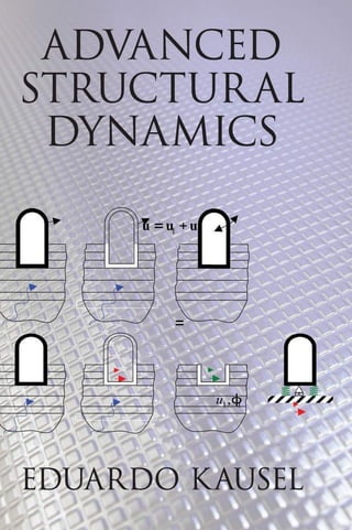
22
22
1 DOF = vertical displacement of mass:
2 DOF = vertical displacement + rotation of mass
2 DOF = rotation of the masses. Even though two translational masses exist, there is no
degree of freedom associated with them, because the supports prevent the motion.
By way of contrast,consider next an inextensible arch with a single lumped mass,as shown.
This system has now 3 DOF because, unlike the beam in the second example above, the
bending deformation of the arch will elicit not only vertical and rotational motion but
also horizontal displacements.
1.8 Modeling Structural Systems
1.8.1 Levels of Abstraction
The art of modeling a structural system for dynamic loads relates to the process by
which we abstract the essential properties of an actual physical facility into an ideal-
ized mathematical model that is amenable to analysis. To understand this process, it is
instructive for us to consider the development of the model in terms of steps or levels
of abstraction.
To illustrate these concepts, consider a two-
story frame subjected to lateral wind loads,
as shown in Figures 1.29 to 1.32. As we shall see, the models for this frame in the first
through fourth levels of abstraction will be progressively reduced from infinitely many
dynamic degrees of freedom, to 12, 8, and 2 DOF, respectively.
In the first level of abstraction, the principal elements of the actual system are iden-
tified, quantified, and idealized, namely its distribution of mass, stiffness, and damp-
ing; the support conditions; and the spatial-
temporal characteristics of the loads. This
preliminary model is a continuous system with distributed mass and stiffness, it spans
m
m, J
m, J m, J
Figure 1.26
Figure 1.25
Figure 1.27
m, J
Figure 1.28

23
p3
p4
p1
p2
u3
u4
u2
u1
w1
w2 w4
θ1
w2
θ3
θ4
θ2
m3, J3
m4, J4
m2, J2
m1, J1
Figure 1.29
Figure 1.30
u1
p1
p2
p3
p4
m2
m3
m4
m1 u3
u4
u2
Figure 1.31

24
24
the full three-
dimensional space, and it has infinitely many degrees of freedom. Of
course, in virtually all cases, such a model cannot be analyzed without further sim-
plifications. However, it is a useful conceptual starting point for the development of
systems that can be analyzed, using some of the techniques that will be described in
the next section.
In the second level of abstraction, we transform the continuous system into a discrete
system by lumping masses at the nodes, and/
or representing the structural elements with
ideal massless elements, such as beams, plates, finite elements, and so forth. We also con-
dense distributed dynamic loads, such as wind pressures, into concentrated, equivalent
forces that act on the nodes alone. We initially allow the structural elements to deform
in a most general fashion; for example, we assume that beams may deform axially, in
bending and in shear.Also, the nodal masses have both translational as well as rotational
inertia, so that nodes could typically have up to six degrees of freedom each. In general,
this system will have a finite, but large number of degrees of freedom. Inasmuch as nodal
coupling occurs only when two or more nodes are connected by a structural element, the
stiffness and damping matrices will be either narrowly banded or sparse. Such a system is
said to be closely coupled. In the example shown, the system has 12 DOF: 8 translational
and 4 rotational DOF.
In a third level of abstraction,we may neglect vertical inertia forces as well as rotational
inertias. Note carefully that this does not imply that the vertical motions or rotations
vanish. Instead, these become static degrees of freedom, and thus depend linearly on
the lateral translations, that is, they become slave DOF to the lateral translations, which
are the master DOF. While the number of dynamic DOF of this model is now less than
in the original one, we pay a price: the stiffness and damping matrices will now be fully
populated, and the system becomes far coupled. In our example, the structure has now
four dynamic degrees of freedom.The process of reducing the number of DOF as a result
of neglecting rotational and translational inertias can formally be achieved by matrix
manipulations referred to as static condensation.
In a fourth and last level of abstraction, we introduce further simplifications by assum-
ing that certain structural elements are ideally rigid, and cannot deform. For example,
2
u1
p1+ p3
p2+ p4
m1+ m3
u2
m2+ m4 Figure 1.32

25
we can usually neglect the axial deformations of beams (i.e., floors), an assumption that
establishes a kinematic constraint between the axial components of motion at the two
ends of the beam. In our example, this means that the horizontal motions at each eleva-
tion are uniform, that is, u1 = u3, u2 = u4. The system has now only 2 DOF. The formal
process by which this is accomplished through matrix manipulations is referred to as kine-
matic condensation.
Once the actual motions u1, u2 in this last model have been determined, it is possible to
undo both the static and dynamic condensations, and determine any arbitrary component
of motion or force, say the rotations of the masses, the axial forces in the columns, or the
support reactions.
1.8.2 Transforming Continuous Systems into Discrete Ones
Most continuous systems cannot be analyzed as such, but must first be cast in the form of
discrete systems with a finite number of DOF.We can use two basic approaches to trans-
form a continuous system into a discrete one.These are
• Physical approximations (Heuristic approach): Use common sense to lump masses,
then basic methods to obtain the required stiffnesses.
• Mathematical methods: Weighted residuals family of methods, the Rayleigh–Ritz
method, and the energy method based on the use of Lagrange’s equations. We cite
also the method of finite differences, which consists in transforming the differential
equations into difference equations, but we shall not consider it in this work.
We succinctly describe the heuristic method in the following, but postpone the power-
ful mathematical methods to Chapter 6, Sections 6.2–
6.4 since these methods are quite
abstract and require some familiarity with the methods of structural dynamics.
Heuristic Method
Heuristics is the art of inventing or discovering.As the definition implies, in the heuristic
method we use informal, common sense strategies for solving problems.
To develop a discrete model for a problem in structural dynamics, we use the following
simple steps:
• Idealize the structure as an assembly of structural elements (beams, plates, etc.),
abstracting the essential qualities of the physical system. This includes making deci-
sions as to which elements can be considered infinitely rigid (e.g., inextensional
beams or columns, rigid floor diaphragms, etc.), and also what the boundary condi-
tions should be.
• Idealize the loading, in both space and time.
• On the basis of both the structural geometry and the spatial distribution of the loads,
decide on the number and location of the discrete mass points or nodes. These will
define the active degrees of freedom.
• Using common sense, lump (or concentrate) the translational and rotational masses
at these nodes. For this purpose, consider all the mass distributed in the vicinity of
the active nodes, utilizing the concept of tributary areas (or volume). For example, in

26
26
the simplest possible model for a beam, we would divide the beam into four equal
segments, and lump the mass and rotational inertia of the two mid-
segments at the
center (i.e., half of the beam), and that of the lateral segments at each support (one
quarter each). In the case of a frame, we would probably lump the masses at the inter-
section of the beams and columns.
• Lump the distributed loads at the nodes, using again the concept of tributary area.
• Obtain the global stiffness matrix for this model as in aTinkertoy, that is, constructing
the structure by assembly and overlap of the individual member stiffness matrices, or
by either the direct stiffness approach or the flexibility approach. The latter is usually
more convenient in the case of statically determinate systems, but this is not always
the case.
• Solve the discrete equations of motion.
1.8.3 Direct Superposition Method
As the name implies, in this method the global stiffness matrix is obtained by assembling
the complete system by superimposing the stiffness matrices for each of the structural ele-
ments. This entails overlapping the stiffness matrices for the components at locations in
the global matrix that depend on how the members are connected together. Inasmuch as
the orientation of the members does not generally coincide with the global directions, it is
necessary to first rotate the element matrices prior to overlapping, so as to map the local
displacements into the global coordinate system. You are forewarned that this method
should never be used for hand computations, since even for the simplest of structures this
formal method will require an inordinate effort. However, it is the standard method in
computer applications, especially in the finite element method.
1.8.4 Direct Stiffness Approach
To obtain the stiffness matrix for the structural system using the direct stiffness approach,
we use the following steps:
• Identify the active DOF.
• Constrain all active DOFs (and only the active DOF!).Thus, in a sense, they become
“supports.”
• Impose, one at a time, unit displacements (or rotations) at each and every one of the
constrained DOF. The force (or moment) required to impose each of these displace-
ments together with the “reaction” forces (or moments) at the remaining constrained
nodes, are numerically equal to the terms of the respective column of the desired
stiffness matrix.
This method usually requires considerable effort, unless the structure is initially so highly
constrained that few DOF remain.An example is the case of a one-
story frame with many
columns (perhaps each with different ending conditions) that are tied together by an
infinitely rigid girder. Despite the large number of members, such a system has only one
lateral DOF, in which case the direct stiffness approach is the method of choice.

27
Let us illustrate this method by means of an example. Consider a structure composed
of a bending beam with two lumped masses, as shown in Figure 1.33. While the masses
can and do rotate, there are no rotational inertias associated with them, so they are
simply static degrees of freedom. Hence, this system has a total of only two dynamic
DOF, namely the lateral translation of the two masses. To determine the elements of the
2 × 2 stiffness matrix, we consider the two test problems shown below, and determine by
some standard method, such as the slope-deflection method, the reactions at the fictitious
supports. Notice that the masses are allowed to rotate freely, since they are not active,
dynamic DOF.
k k
k k
k
k
k k
k k
11 12
21 22
11
21
11 12
21 22
1
0
0












=











 1
1
12
22






=






k
k
(1.22)
1.8.5 Flexibility Approach
The flexibility approach is basically the converse of the direct stiffness approach, and
leads to the inverse of the stiffness matrix, which is the flexibility matrix. It is particularly
well suited for statically determinate structures, but may require considerable effort if the
structure is indeterminate.
The discrete flexibility matrix is obtained as follows:
• Identify the active DOF.
• Apply, one at a time, a unit force (or moment) at each and every active DOF. The
observed displacements (or rotations) at all active DOF are then numerically equal to
the columns of the flexibility matrix.The stiffness matrix, if desired, must be obtained
by inversion of the flexibility matrix.
To illustrate this method, consider once more the example of the previous section.
Without constraining the structure, we now solve for the displacements produced by the
u = 1
k21
k11
k22
k12
u = 1
Figure 1.33. Direct stiffness method.

28
28
two test loadings shown in Figure 1.34.These displacements are numerically equal to the
elements of the flexibility matrix. Since the cantilever column is statically determinate,
this problem is particularly simple to solve, either from tabulated formulae (e.g., see the
section“Stiffnesses of SomeTypical Linear Systems”),or by standard methods such as the
conjugate beam method.
f f
f f
f
f
f f
f f
11 12
21 22
11
21
11 12
21 22
1
0
0












=











 1
1
12
22






=






f
f
(1.23)
Example 1
Consider a simply supported, homogeneous bending beam subjected to a dynamic load
at the center, as shown in Figure 1.35.Although this structure can be analyzed rigorously
as a continuous system, we shall pretend ignorance of this fact, and attempt instead to
represent it as a discrete system. Clearly, the absolute simplest representation is a mass-
less beam with a concentrated mass lumped at the location of the load equal to mass of
the shaded (tributary) area, that is, m AL
= 1
2 ρ .The remaining mass may be lumped at the
supports, but because they do not move, they have no effect on the discrete model. This
assumes that the temporal variation of the load changes no faster than the beam’s funda-
mental period.
From the flexibility approach, a unit static load at the center causes a displacement
f L EI
= 1
48
3
/ , so the stiffness of this 1-
DOF system is k f EI L
= =
1 48 3
/ / .
Example 2
By way of contrast, consider next the same problem subjected to two dynamic loads,
as shown in Figure 1.36. A satisfactory dynamic model would involve now two or more
masses, particularly if the loads are negatively correlated, that is, if p t p t
2 1
( ) ~ ( )
− .
Each of the three lumped masses now equals one-
fourth of the total beam mass, while
the elements of the 3 × 3 flexibility matrix can readily be obtained from the formula for
deflections listed in the section on typical linear systems.
p1 =1
f21
f11
p2 =1
f22
f12
Figure 1.34. Flexibility method.

29
Example 3
As a last example, consider a horizontally layered soil subjected to vertically propagat-
ing shear waves (i.e., SH-
waves). Inasmuch as motions in horizontal planes are uniform,
it suffices to consider a column of soil of unit width and subjected to pure shear. We
begin by discretizing the soil column into elements j = 1, 2, 3… of unit cross section
(Aj = 1) whose thickness hj is small in comparison to the typical wavelengths in the seis-
mic motion.
Using the heuristic approach, we obtain lumped masses and discrete springs whose
values are
m h h
j j j j j
= +
− −
1
2 1 1
( )
ρ ρ (1.24)
k
G
h
C
h
j
j
j
j sj
j
= =
ρ 2
(1.25)
The mass and stiffness matrices are then
M K
= { } =
−
− + −
− −
− +



−
− −
diag ,
m m m
k k
k k k k
k k
k k k
n
n
n n n
1 2
1 1
1 1 2 2
2 1
1 1













1.8.6 Viscous Damping Matrix
Damping forces in a mechanical system result from various phenomena that lead to
internal energy dissipation in the form of heat. These arise as a result of nonrecoverable
processes associated with material hysteresis, drag, or friction. A particularly simple dis-
sipation mechanism is in the form of linear, viscous damping, in which damping forces are
proportional to the rate of material deformation, that is, to the velocity of deformation.
Although most structural systems exhibit damping forces that are not of a viscous nature,
it is nevertheless often convenient to approximate these as being of the viscous type.
p(t) p(t)
Figure 1.35. Mass lumping.
p1(t) p2(t) p1(t) p2(t)
Figure 1.36

30
30
The motivation for this lies in the great mathematical simplification that linear viscous
damping confers to the idealized structural system, and the good approximations that
can still be achieved whatever the actual damping type. Thus, in a way the main reason
for using viscous damping is that “we can get away” with it, and much less so because it is
convenient. Here we show how to construct damping matrices for an assembly of viscous
dashpots, and shall defer the treatment of nonviscous damping and the formulation of
appropriate nonviscous damping models to later sections.
A viscous dashpot (or shock absorber) is a mechanical device in which the force neces-
sary to produce a deformation is proportional to the velocity of deformation. Damping
forces that are proportional to the velocity of deformation are said to be viscous. In gen-
eral, the assembly of damping elements follows the same formation rules as those for
stiffness elements. Hence, viscous damping matrices have a structure that is similar to that
of stiffness matrices. Consider, for example, a system consisting of two spring–
dashpot
systems in series subjected to forces p1, p2 that produce time-
varying displacements u1, u2.
The stiffness and damping matrices are
K =
−
− +






k k
k k k
1 1
1 1 2
(1.26)
hj Gj ρj
1
1
Rigid base
Layer
1
2
n
. . .
kj
mj
hj
Figure 1.37. Column of soil subjected to SH waves.

31
C =
−
− +






c c
c c c
1 1
1 1 2
(1.27)
and the force-
deformation equations is
p Cu K u u p
( )
t
u
u
p
p
= + =






=






 1
2
1
2
(1.28)
Then again, most structures do not have dashpots, in which case C cannot be assembled
a priori.
1.9 Fundamental Dynamic Principles for a Rigid Body
1.9.1 Inertial Reference Frames
Consider a free, rigid body whose motion is being observed in a global or Newtonian
inertial reference frame with unit base vectors ˆ , ˆ , ˆ
e e e
1 2 3. Fixed to this body at its center of
mass is a set of local coordinate axes with unit base vectors ˆ , ˆ , ˆ
g g g
1 2 3at which the motions
(translations and rotations) elicited by an external force f and torque t are measured.The
body has total mass m and a symmetric rotational inertia tensor J g g
= Jij i j
ˆ ˆ (summation
over repeated indices implied), whose components are
J r dV x x dV
ij ij
Vol
i j
Vol
= −
∫ ∫
δ ρ ρ
2
(1.29)
in which δij is the Kronecker delta, r x x x
2
1
2
2
2
3
2
= + + , and the coordinates xi are relative to
the center of mass. The diagonal terms are the mass moments of inertia, while the off-
diagonal terms are the products of inertia; notice the negative sign in front of the second
integral. If the axes are principal, then the products of inertia vanish, and only the diago-
nal terms remain.
1.9.2 Kinematics of Motion
Consider a rigid body that moves and rotates in some arbitrary fashion, and within this
body, choose as reference point the center of mass, which moves with velocity v and about
which the body rotates with instantaneous angular velocity ω. We also choose another
arbitrary observation point p on the body whose position relative to the reference point is
r r
= ( )
t , and whose velocity is vp. From vector mechanics, the following holds:
d
dt
r r
= ×
ω (1.30)
k2
c2
k1
c1
u2, p2 u1, p1
Figure 1.38

32
32
v v r
p = + ×
ω (1.31)
a a r r
p = + × + × ×
( )
α ω ω (1.32)
in which α ω
=  is the angular acceleration, ω ω ω ω
× ×
( ) = •
( )−
r r r
ω2
and ω2
= •
ω ω. Now,
the position vector r can be expressed either in local (rotating) or global (nonrotating)
coordinates with unit orthogonal basis vectors ĝi and êi, respectively, that is,r g e
= ′ =
x x
i i i i
ˆ ˆ .
In particular, if we choose one of the rotating basis vectors r g e
= =
ˆ ˆ
i ij j
γ , in which the γ ij
are the direction cosines of the rotated basis with respect to the global basis, then
d
dt i i
d
dt ij j ij kj k
ˆ ˆ ˆ ˆ
g g e g
= × = =
ω γ γ γ
 (1.33)
or in matrix format
d
dt
ˆ
ˆ
ˆ
ˆ
g
g
g
1
2
3
3 2
3 1
2 1
0
0
0










=
′ − ′
− ′ ′
′ − ′










ω ω
ω ω
ω ω
g
g
g
g
1
2
3
11 12 13
21 22 23
31 32 33
ˆ
ˆ










=


  
  
  
γ γ γ
γ γ γ
γ γ γ






















γ γ γ
γ γ γ
γ γ γ
11 21 31
12 22 32
13 23 33
1
2
3
ˆ
ˆ
ˆ
g
g
g








= 
R R G
T
(1.34)
The local components of the angular velocity vector are then
′ = + +
ω γ γ γ γ γ γ
1 21 31 22 32 23 33
   (1.35)
′ = + +
2 31 11 32 12 33 13
   (1.36)
′ = + +
3 11 21 12 22 13 23
   (1.37)
Cardanian Rotation
The rotation of a rigid body rotation in 3-
D space can be described in terms of three
independent, right-
handed rotations about the local coordinate axes or Cardanian angles
θ θ θ
1 2 3
, , whose sequence must remain inviolate. Of various possible choices, we choose
the following rule:
• Rotate about the global x-
axis by an angle θ1, which moves the axes to, say, posi-
tion
  
x y z
, , .
• Rotate about the local

y by an angle θ2, which moves the axes to position   
x y z
, , .
• Rotate about the local 
z axis by an angle θ3 which moves the axes to their final posi-
tion ′ ′ ′
x y z
, , .
The three rotation matrices needed to accomplish these three sequential elementary
rotations are
ê1
ê2
ê3
ĝ1
ĝ2
ĝ3
p
v
r
ù
vp
Figure 1.39

33
R R
1 1 1
1 1
2
2 2
1 0 0
0
0
0
0 1
=
−










=
−
cos sin
sin cos
,
cos sin
s
θ θ
θ θ
θ θ
i
in cos
,
cos sin
sin cos
θ θ
θ θ
θ θ
2 2
3
3 3
3 3
0
0
0
0 0 1










= −







R





(1.38)
Observe the different signs of the off-diagonal terms for R2.With the shorthand cj j
= cosθ ,
sj j
= sinθ we obtain the complete rotation matrix as
R R R R
= =
+ −
− − +
3 2 1
2 3 1 3 1 2 3 1 3 1 2 3
2 3 1 3 1 2 3 1 3 1
c c c s s s c s s c s c
c s c c s s s s c c s
s s
s s c c c
ij
T
2 3
2 1 2 1 2
−










= { } ′ = = ′
γ , ,
x R x x R x (1.39)
This matrix contains the direction cosines γ ij of the local axes with respect to the global
axes. Using the preceding expressions together with MATLAB®
’s symbolic manipulation
capability, it can be shown that the components of the angular velocity vector are given by
′ = +
ω θ θ θ θ θ
1 1 2 3 2 3
 
cos cos sin (1.40)
′ = −
ω θ θ θ θ θ
2 2 3 1 2 3
 
cos cos sin (1.41)
′ = +
ω θ θ θ
3 3 1 2
  sin (1.42)
Eulerian Rotation
The most common alternative approach to describe rotations is by means of the so-
called
Eulerian angles, which differ from the Cardanian rotations in that one local axis is used
twice. These angles can be visualized as follows. Assume that initially, the local axes with
unit base vectors ˆ , ˆ , ˆ
g g g
1 2 3 and the global axes with unit base vectors ˆ , ˆ , ˆ
e e e
1 2 3 coincide in
space.Thereafter, carry out the following three rotations (right-
hand rule applies, and the
sequence must remain inviolate):
• Rotate the local frame about the vertical axis ĝ3 by a horizontal angle (azimuth, or
longitude) 0 2
≤ ≤
φ π until the plane x z
, (i.e., ˆ , ˆ
g g
1 3) contains the line from the center
to the final north pole. Of the two possible rotations, which differ by 180 degrees,
choose the one for which the angular distance (about ĝ2) from the initial to the final
north poles satisfies 0 ≤ ≤
θ π.
• Rotate next the local frame about ĝ2 through a right-
handed angle 0 ≤ ≤
θ π. This
brings ĝ3 to its final position, so cosθ = ⋅
g e
 
3 3.
• Finally, rotate again the local frame about ĝ3 by an angle 0 2
≤ ≤
ψ π. This brings the
local system to its ultimate configuration.
If G g e
= { }= ⋅
{ }
γ ij i j
ˆ ˆ is the matrix of direction cosines for the three local axes, then its ele-
ments γ ij in terms of the Eulerian angles are as shown in Table 1.3.1
In local body coordinates, the components of the rotational velocity vector ω are then
ω θ ψ φ θ ψ
1 = −
 
sin sin cos (1.43)
1
J. L. Synge and B. A. Griffith, Principles of Mechanics (New York: McGraw-Hill, 1959), 261.

34
34
ω θ ψ φ θ ψ
2 = +
 
cos sin sin (1.44)
ω φ θ ψ
3 = +
 
cos (1.45)
1.9.3 Rotational Inertia Forces
Let’s now examine the rotational inertia forces in a body.For this purpose,let J denote the
rotational inertia tensor, which can be written in local or global coordinates (Note: Pairs
of juxtaposed basis vectors constitutes a dyad, and repeated indices imply summation.)
J g g e e
= ′ =
J J
ij i j ij i j
ˆ ˆ ˆ ˆ (1.46)
In local coordinates, the components ′
Jij of J are time invariant, so
d
dt ij
d
dt i j i
d
dt j ij i j i j
J J
J g g g g g g g g
= ′ +
( )= ′ × + ×
( )
= × ′
ˆ ˆ ˆ ˆ ˆ ˆ ˆ ˆ
ω ω
ω J
J J
ij i j ij i j
ˆ ˆ ˆ ˆ
g g g g
J J
− ′ ×
= × − ×
ω
ω ω
(1.47)
Now, the principle of conservation of angular momentum states that the external moment
(or torque) t is given by the rate of change of the angular momentum h J
= •É, that is,
t h J J J J J J
J J
= = •
( ) = ( )• + • = × − ×
( )• + •
= • + × •
d
dt
d
dt
d
dt
d
dt
ω ω ω ω ω ω α
α ω ω
(1.48)
This is because J 0
× •
ω ω = . Notice also that h J J
= • = •
ω ω , because J is symmetric.
Expressing next the various terms in the expression above by means of the local (moving)
unit vectors, we obtain
J g g g g J g g
• ′ • ′ = ′ ′ • = ′ ′ = ′ ′
ω α
= J J J J
ij i j k k ij j i ij j i ij j
ˆ ˆ ˆ ˆ , ˆ ˆ
ω ω α ω
 i
i (1.49)
Furthermore, if the moving axes attached to the rigid body are principal axes, then
only the diagonal terms of the inertia tensor exist, so J g g g
• ′ ′ + ′ ′ + ′ ′
ω= J J J
11 1 1 22 2 1 33 3 3
ω ω ω
ˆ ˆ ˆ .
Hence,
ω ω
× •
( ) ′ ′ ′
′ ′ ′ ′ ′ ′
= ′ − ′
(
J
g g g
=
ˆ ˆ ˆ
1 2 3
1 2 3
11 1 22 2 33 3
33 22
ω ω ω
ω ω ω
J J J
J J )
) ′ ′ + ′ − ′
( ) ′ ′ + ′ − ′
( ) ′ ′
ω ω ω ω ω ω
2 3 1 11 33 3 1 2 22 11 1 2 3
ˆ ˆ ˆ
g g g
J J J J (1.50)
t g
= ′ ′ + ′ − ′
( ) ′ ′

 
 + ′ ′ + ′ − ′
( ) ′ ′
J J J J J J
11 1 33 22 2 3 1 22 2 11 33 3
α ω ω α ω
ˆ ω
ω α ω ω
1 2 33 3 22 11 1 2 3

 
 + ′ ′ + ′ − ′
( ) ′ ′

 

ˆ ˆ
g g
J J J
(1.51)
Table 1.3. Direction cosines of local axes in terms of Eulerian angles
cos cos cos sin sin
θ φ ψ θ ψ
− cos sin cos sin cos
φ ψ θ φ ψ
+ −sin cos
θ ψ
− −
cos cos sin sin cos
θ φ ψ φ ψ cos cos cos sin sin
φ ψ θ φ ψ
− sin sin
θ ψ
sin cos
θ φ sin sin
θ φ cosθ

Advanced Structural Dynamics - Eduardo Kausel

Advanced Structural Dynamics - Eduardo Kausel

Recommended

Recommended

More Related Content

What's hot

What's hot (20)

Similar to Advanced Structural Dynamics - Eduardo Kausel

Similar to Advanced Structural Dynamics - Eduardo Kausel (20)

More from TheJamez

More from TheJamez (20)

Recently uploaded

Recently uploaded (20)

Advanced Structural Dynamics - Eduardo Kausel