This document provides an overview of wireless communication technologies for IoT networks. It evaluates long range and short range technologies like Sigfox, LTE-M, and ZigBee in terms of capacity and coverage. It also analyzes the performance of a ZigBee network in indoor and outdoor scenarios with interference from WiFi and Bluetooth. Outdoor tests show fading signals have the biggest impact on path loss, increasing it by 14.8 dB at 0.5 meter antenna heights. Indoor interference from WiFi results in only a 10% packet loss ratio in the worst case scenario of 20 meters between nodes and 5 concrete walls.

3. iii
Supervisors:
Henrik Lehrman Christiansen – Associate Professor, Ph.D
Matteo Artuso – Ph.D student

4. iv
Abstract
The emerging IoT networks will present numerous challenges in developing
compatible protocols and communication technologies that will fulfil the requirements
imposed by M2M communications and low power wide area networks. Long range
and short range wireless communication technologies are evaluated in this report
with the purpose of providing an analysis on capacity and coverage for Sigfox,
LTE-M and ZigBee. Finally the coverage performance of a ZigBee network is
evaluated in indoor and outdoor scenarios with interference patterns from IEEE
802.11b/g/n and Bluetooth. The results show that WiFi interference does not
present a severe impact on the packet delivery ratio with only 10% lost packets
in a heavy indoor WiFi network usage in the worst case scenario of 20 meters
between nodes and 5 concrete walls. Outdoor results show that the biggest impact
comes from fading signals and the path loss is increased with 14.8 dB for antenna
heights at 0.5 meters. The outdoor tests also evaluated the impact of rain on the
wireless 2.4 GHz signal which resulted in only 6 dB increased path loss.

5. v
Table of contents
TABLE OF CONTENTS V
1 INTRODUCTION 1
1.1 INTERNET OF THINGS 1
1.2 M2M COMMUNICATION 2
1.3 MOTIVATION 2
OBJECTIVE 2
SCOPE 2
JUSTIFICATION 2
1.4 REPORT STRUCTURE 3
2 WIRELESS COMMUNICATION NETWORKS 4
2.1 SENSOR NETWORKS 4
2.2 WIRELESS NETWORKS 6
WIRELESS SENSOR NETWORKS 7
ZIGBEE 8
BLUETOOTH-LE 11
2.3 CELLULAR NETWORKS 14
2G 15
3G 17
LTE/4G 19
2.3.3.1. LTE-M 20
2.4 LOW POWER WIDE AREA NETWORKS 22
IOT ARCHITECTURE 23
WEIGHTLESS 25
SIGFOX 27
2.5 SUMMARY 29
3 THROUGHPUT, CAPACITY AND COVERAGE INVESTIGATIONS 31
3.1 IOT PROTOCOLS 31
3.2 ERRORS IN WIRELESS COMMUNICATION 33
3.3 LINK BUDGET 36
3.4 CAPACITY AND COVERAGE ANALYSIS 43
SIGFOX 44
LTE-M 46
ZIGBEE 47
3.5 SCALABILITY 50
3.6 SUMMARY 51
4 WIRELESS SENSOR NETWORK IMPLEMENTATION 53

6. vi
4.1 RELATED WORK 53
4.2 NETWORK OVERVIEW AND IMPLEMENTATION 56
4.3 SUMMARY 57
5 ZIGBEE COVERAGE PERFORMANCE 58
5.1 RANGE TEST 58
RANGE TEST TOOL 59
5.2 OUTDOOR TESTS 62
BASELINE TEST 62
BLUETOOTH INTERFERENCE 65
EFFECTS OF LIGHT RAIN AND FADING SIGNALS ON THE ZB NETWORK 68
5.3 INDOOR TESTS 72
IDLE WIFI NETWORK INTERFERENCE 72
BUSY WIFI NETWORK INTERFERENCE 74
5.4 SUMMARY 77
6 CONCLUSIONS 79
6.1 FUTURE WORK 80
7 BIBLIOGRAPHY 81

7. FIGURE 1 SENSOR NODE ARCHITECTURE 5
FIGURE 2 SENSOR NETWORK ARCHITECTURE/STAR TOPOLOGY 6
FIGURE 3 WSN LOCAL AREA COVERAGE AND WIDE AREA COVERAGE 7
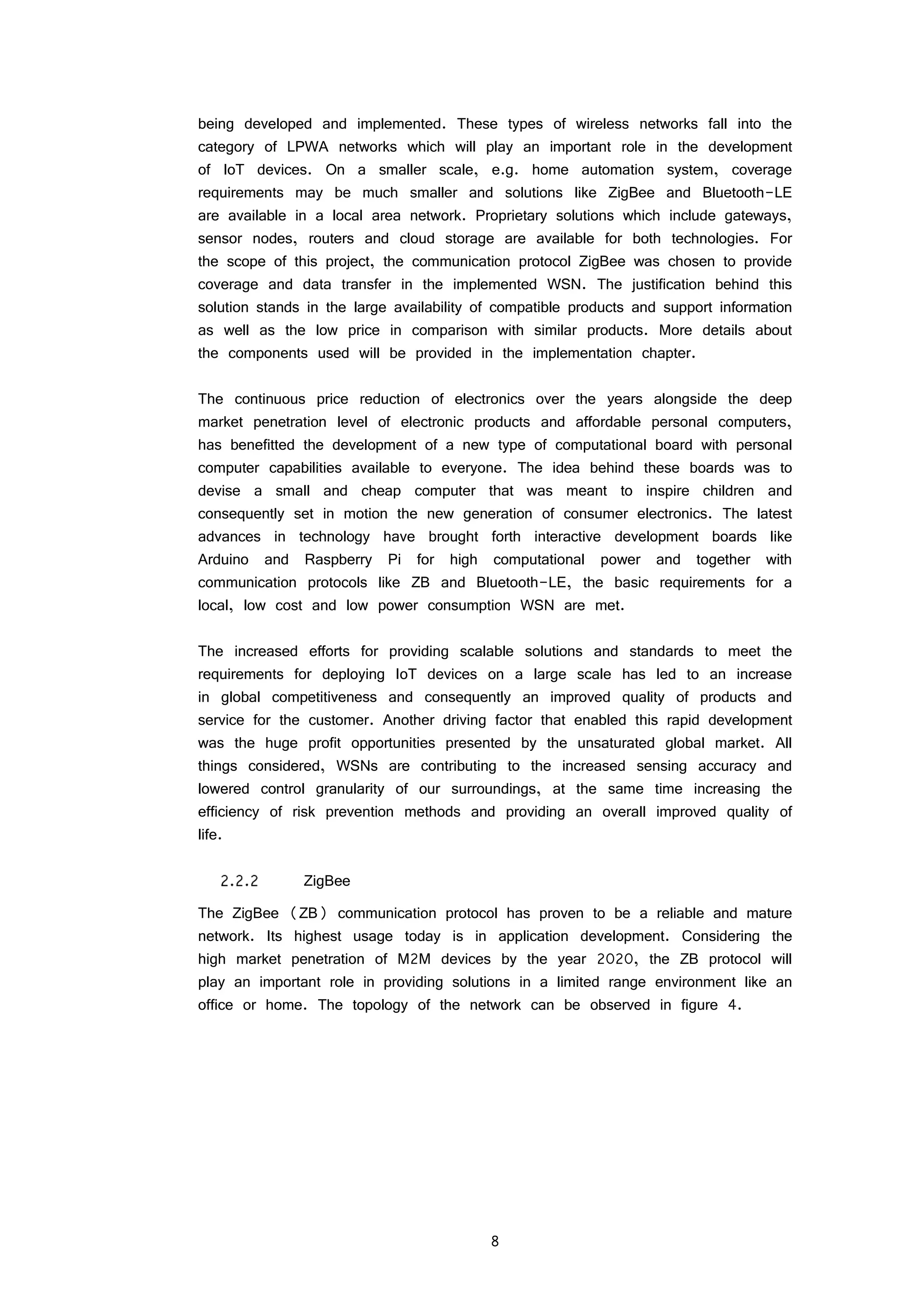
FIGURE 4 ZIGBEE NETWORK TOPOLOGY 9
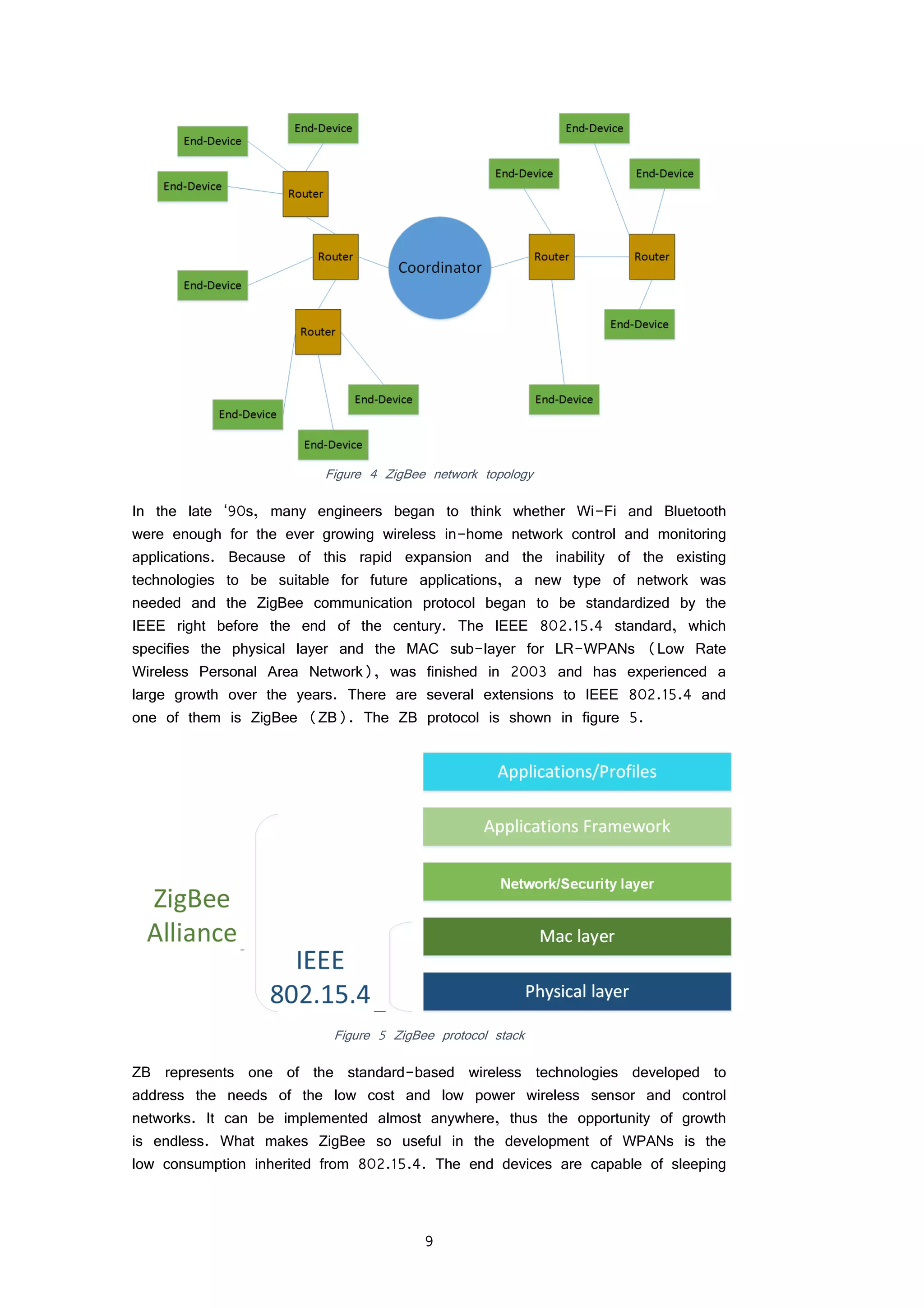
FIGURE 5 ZIGBEE PROTOCOL STACK 9
FIGURE 6 BLUETOOTH LE STACK 12
FIGURE 7 GLOBAL MOBILE DATA TRAFFIC, 2014-2019 [34] 14
FIGURE 8 GSM NETWORK ARCHITECTURE 16
FIGURE 9 GPRS ARCHITECTURE 17
FIGURE 10 UMTS NETWORK ARCHITECTURE 18
FIGURE 11 LTE NETWORK ARCHITECTURE 20
FIGURE 12 LPWA NETWORK DEPLOYMENT SCENARIOS 23
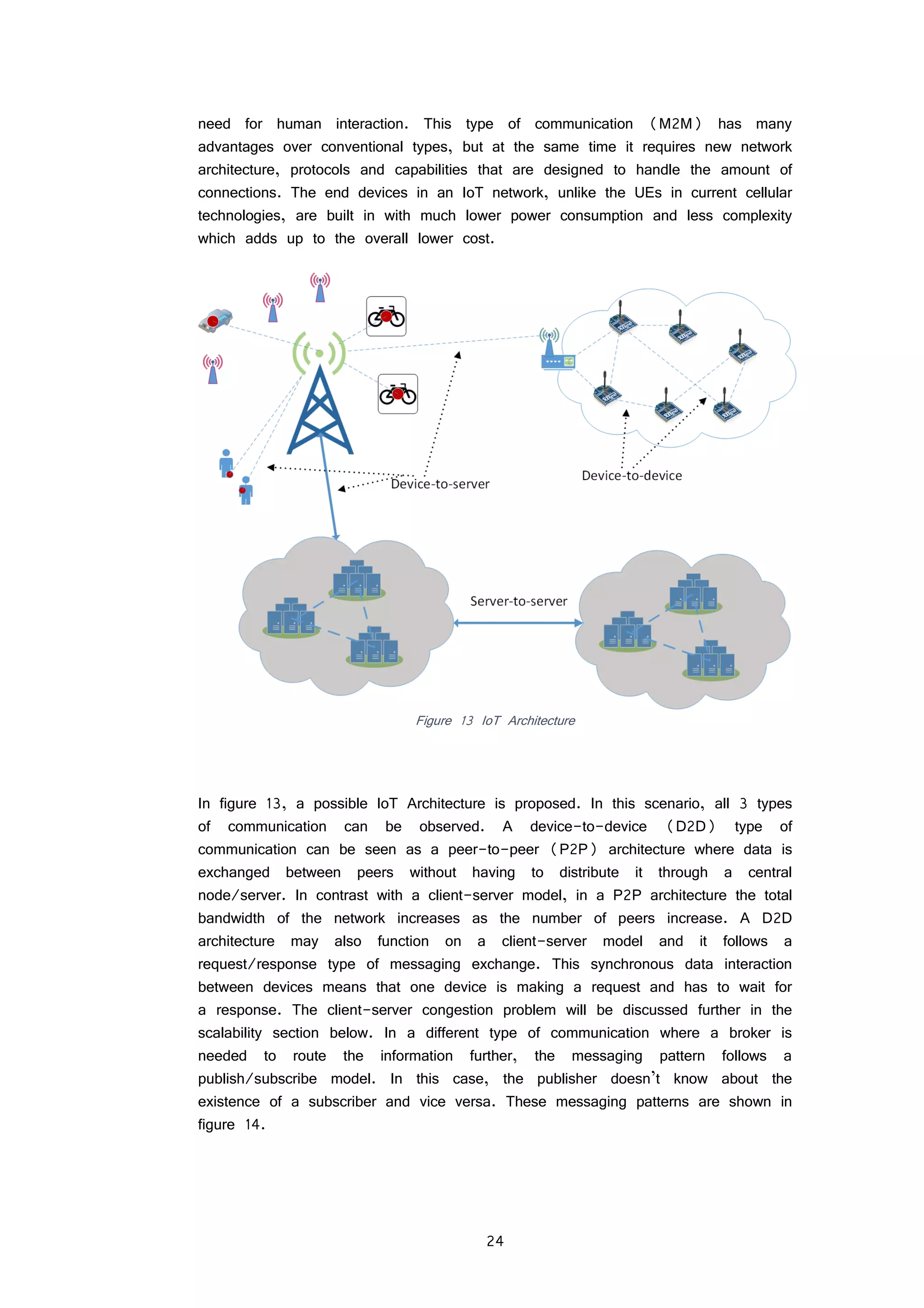
FIGURE 13 IOT ARCHITECTURE 24
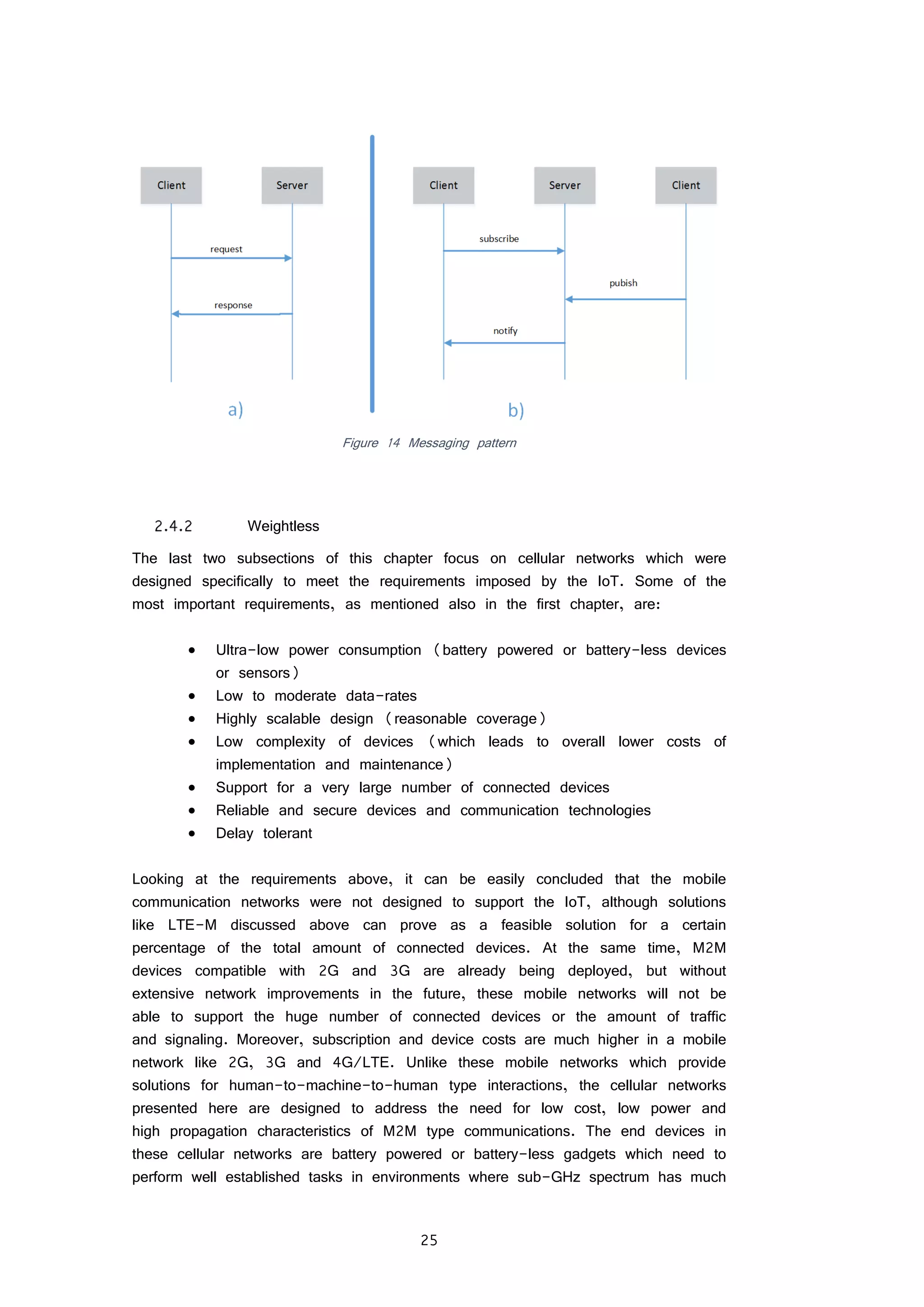
FIGURE 14 MESSAGING PATTERN 25
FIGURE 15 WEIGHTLESS NETWORK ARCHITECTURE 27
FIGURE 16 SIGFOX USE CASE 28
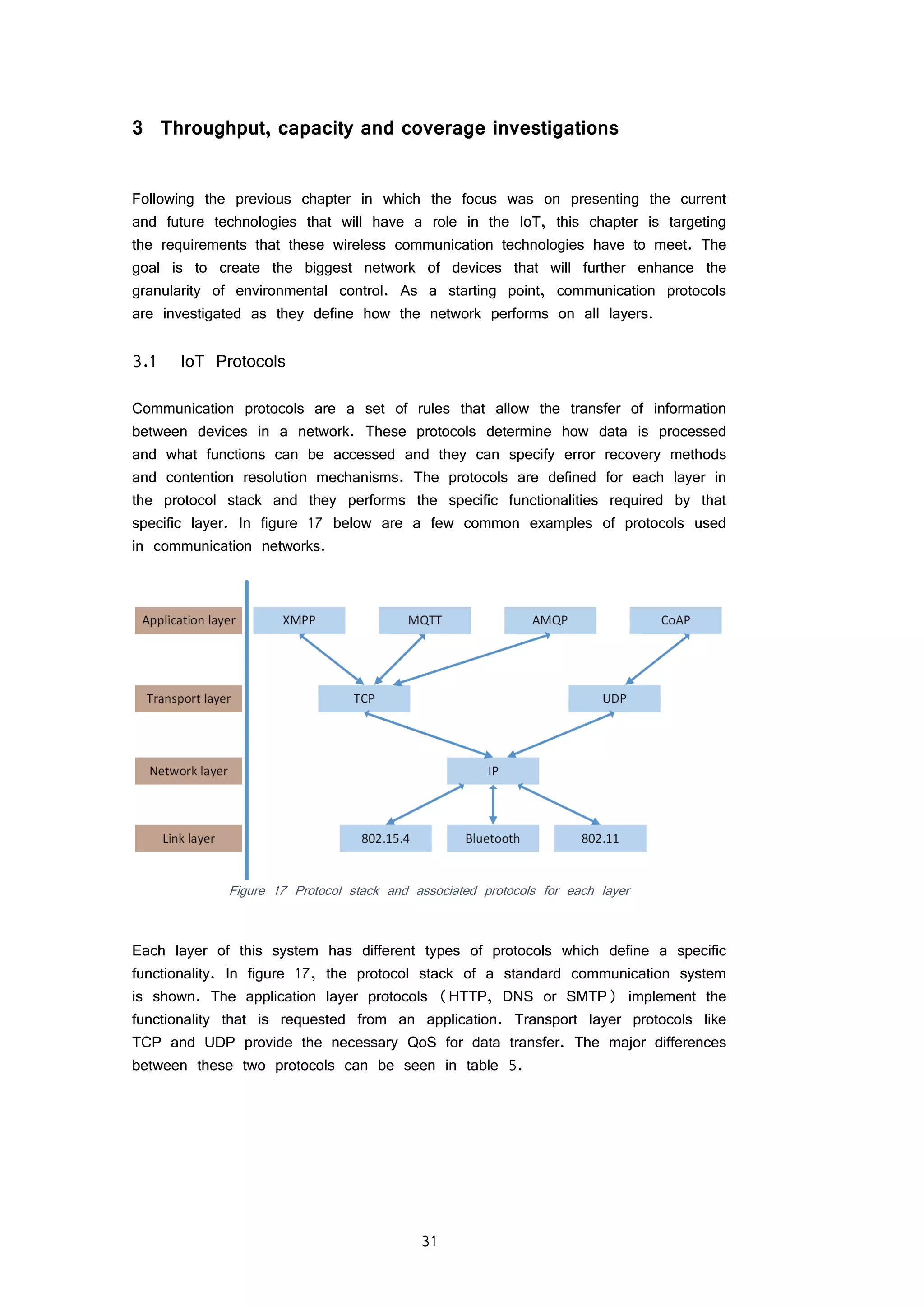
FIGURE 17 PROTOCOL STACK AND ASSOCIATED PROTOCOLS FOR EACH LAYER 31
FIGURE 18 BER FOR BPSK AND IN RAYLEIGH AND AWGN CHANNELS 35
FIGURE 19 BER FOR A BPSK AND QPSK SIGNAL IN AN AWGN CHANNEL 36
FIGURE 20 FREE SPACE PATH LOSS IN 900 MHZ AND 2.4 GHZ BANDS 38
FIGURE 21 OKUMURA HATA PATH LOSS MODEL FOR 900 MHZ FOR SEVERAL SCENARIOS WITH DIFFERENT
ANTENNA HEIGHTS [M] 39
FIGURE 22 OKUMURA HATA PATH LOSS MODEL FOR 2.4 GHZ FOR SEVERAL SCENARIOS WITH DIFFERENT
ANTENNA HEIGHTS [M] 39
FIGURE 23 INDOOR PATH LOSS FOR 900 MHZ AND 2.4 GHZ BANDS 41
FIGURE 24 RANGE COMPARED WITH DATA RATE CONSIDERING DIFFERENT TECHNOLOGIES 43
FIGURE 25 COVERAGE ENHANCEMENTS FOR REL-13 LTE M2M DEVICES 47
FIGURE 27 WIRED CONNECTION FROM METERING DEVICE TO RPI 53
FIGURE 28 WIRELESS CONNECTIVITY BETWEEN RPI AND SENSOR 54
FIGURE 29 DATA ACQUISITION DATABASE [13] 55
FIGURE 30 SYSTEM OVERVIEW 56
FIGURE 31 ZIGBEE TEST CONDITIONS 59
FIGURE 32 X-CTU DEVICE SELECTION 60
FIGURE 33 CLUSTER ID 0X12 MODE OF OPERATION 60
FIGURE 34 X-CTU SESSION CONFIGURATION 61
FIGURE 35 XCTU CHART WITH RSSI AND PDR 61
FIGURE 36 XCTU INSTANT RSSI VALUES 62
FIGURE 37 XCTU PDR 62
FIGURE 38 DECREASING RSSI VALUES IN BASELINE ZB TEST FOR SEVERAL DISTANCES 64
FIGURE 39 THEORETICAL FSPL COMPARED WITH MEASURED AVERAGE RSSI VALUES FOR ALL PACKETS LENGTHS
64
FIGURE 40 DECREASING RSSI VALUES IN BL INTERFERENCE TEST FOR SEVERAL DISTANCES 66
FIGURE 41 AVERAGE RSSI FOR BASELINE TEST COMPARED WITH BL INTERFERENCE 67
FIGURE 42 DIFFERENCE IN AVERAGE RSSI AT 5, 25 AND 50 M FOR BASELINE TEST AND RAIN 69
FIGURE 43 COMPARISON BETWEEN THEORETICAL FSPL, BASELINE PATH LOSS AND FADING PATH LOSS DURING
RAIN 70
FIGURE 44 COMPARISON BETWEEN THEORETICAL FSPL, BASELINE PATH LOSS, FADING PATH LOSS WITH AND
WITHOUT RAIN 71
FIGURE 45 RSSI MEASURED VALUES FOR INDOOR TEST WITH IDLE WIFI NETWORK INTERFERENCE 74

8. viii
FIGURE 46 RSSI VALUES FOR INDOOR TEST WITH BUSY WIFI NETWORK INTERFERENCE 75
FIGURE 47 DIFFERENCE IN RSSI FOR THE IDLE AND BUSY WIFI PERIODS 76
FIGURE 48 COMPARISON OF PATH LOSS FOR THE WIFI INTERFERENCE TESTS 77

9. 1 Introduction
Ever since the development of long distance communication, the focus was on
how to send more information in an efficient way and how to do it faster, cheaper
and more reliable. The first mediums of transmitting information were through cables
and the electric telegraph played an important role in exchanging information in
the industrial era. The arrival of radio technology represented a big step in the
evolution of wireless communication and the efficiency of mobile networks today is
an example of the exponential growth of this technology throughout the 20th
century
and the beginning of the 21st
. Initially, the focus of radio communication was on
transmitting voice messages in the form of analogue signals in the first generation
of mobile networks, but with the development of digital communication, the 2nd
generation allowed the transmission of data. This represented another big step in
the information era where data exchange has been prioritized over voice
communication for the purpose of reliably transmitting high volumes of data in a
short amount of time. The 4th
generation of mobile networks are an example of
high speed data transmission with data rates of up to 300 Mbps. The success
of mobile networks and the availability of an internet connection in most of the
countries around the world has led to the need of connecting more internet capable
devices that could provide valuable information without the need for human
interaction. This new concept of internet connectivity was called the Internet of
Things (IoT).
1.1 Internet of Things
The term “Internet of Things” was coined by Kevin Ashton in 1999. It refers to
the intercommunication of devices within a network and across networks without
the need for human interaction. This kind of network can have a big impact in
many sectors like health care, automotive, transportation and home automation and
it represents a big step in providing a low cost solution to a better quality of life.
Although the focus is on developing wireless technologies that can support such a
large number of devices, several barriers have the potential to slow the development
of the IoT. The three largest are the deployment of IPv6, power for sensors, and
agreement on standards. [36].
Key requirements that a technology must meet in order to sustain the billions of
devices that will be connected in the IoT network are as follows:
 Highly scalable design
 Very low power consumption of end devices
 Large coverage and increased signal penetration

10. 2
The requirement of IoT devices to communicate without the need of human
interaction has led to the development of a new type of machine communication
which is explained in the next subsection.
1.2 M2M communication
Machine to Machine (M2M) communication is one of the main facilitators of IoT
networks. In order to have an efficient and cost effective network, it is imperative
that these devices can communicate between themselves without any human
interaction. Current mobile technologies are not designed to integrate such devices
which require very low power consumption in order to provide functionality for an
extensive period of time (up to 10 years). A few technologies are being developed
today that focus on providing a low cost solution and very scalable design in
order to support the high data volume generated by these devices.
1.3 Motivation
The motivation to proceed with developing this project was born out of the curiosity
to know more about the role of sensor networks and the functionality of the
protocols that facilitate the transfer of low data rates in the IoT.
Objective
The objective of the project entitled “Sensing and controlling the environment using
mobile network based Raspberry Pis” is to provide a series of results based on
experiments took after the implementation process. These results and discussions
are meant to give the reader an overview about the capabilities of the tested
network in a scenario meant to address the IoT. In addition to these results, other
competitive technologies are analyzed and an assessment on the performance of
these technologies is compared in order to determine the best solutions for providing
connectivity to billions of devices in the IoT network.
Scope
The scope of this project is to evaluate the performance of a ZigBee network
regarding coverage and associated PDR (Packet Delivery Ratio) in different
environments.
Justification
The reason for researching this area of wireless networks stands in the fact that
there is a need for providing solutions to the IoT. It is estimated that by 2020
there will be more than 20 billion devices connected in the IoT network [36].
The latest technological advances in wireless technology as well as improvements
in the overall power consumption of such a system have been the missing key
elements in deploying low rate, low power wide area networks on a global scale.

11. 3
1.4 Report Structure
The report follows a well-defined structure in which the theoretical considerations
and presented first followed by an analysis on communication protocols, errors in
wireless communication networks and a comparison on the capacity and coverage
of some technologies that will support the IoT. The report then describes the
implementation of the sensor network necessary for collecting the results which are
discussed in the final part of the report.

12. 4
2 Wireless communication networks
In a general sense, networks have existed long before the introduction of the first
computer network. A group of people with common interests could be also called
a network of people or anything that is connected to something and/or dependent
on something could basically be a network. In the current report, the networks
that are of interest are wireless communication networks. This chapter’s focus is
on presenting the theoretical aspects relevant to understanding the project and its
results.
Sensor networks, as its name suggests, are networks in which end points are
sensors. These are usually deployed in scenarios where there is a constant need
to monitor certain processes in a system. The development of IoT devices has
made sensor networks to be deployed on a much larger scale. These networks
can now be regularly found inside a home, throughout a city or on a farm.
Wireless networks work in a similar way with mobile networks, but they generally
operate on unlicensed frequency bands and are used for data communication. The
most common standard in use today is the IEEE 802.11 (WiFi). Wireless networks
today represent a viable solution for offloading the huge amounts of traffic that
pass through the mobile networks. It is estimated that by 2019, most of the VoIP
data will be transferred over wireless networks [36]. Driven by the huge market
represented by the rapid growing IoT devices, standardization efforts are increasing
and many proprietary solutions for wireless networks based on M2M devices are
emerging. Low Power Wide Area (LPWA) networks will play a major role in
providing a backup solution for the billions of M2M devices.
Wireless communication networks have been a part of everyday life for a few
decades. Like most technological advances, in the beginning it was a very small
portion of the population who could afford a device capable of wireless
communication (e.g. mobile phone). Nowadays a mobile phone has become a
necessity in most places around the world. Cellular networks have facilitated mobile
communication to a global scale for a long time and continue to improve
exponentially in order to supply the current demand of quality services worldwide.
Mobile networks support both voice and data communication in contrast with only
data services in general wireless networks. Also in this section, the impact on
mobile data traffic of wearable and M2M devices is explored.
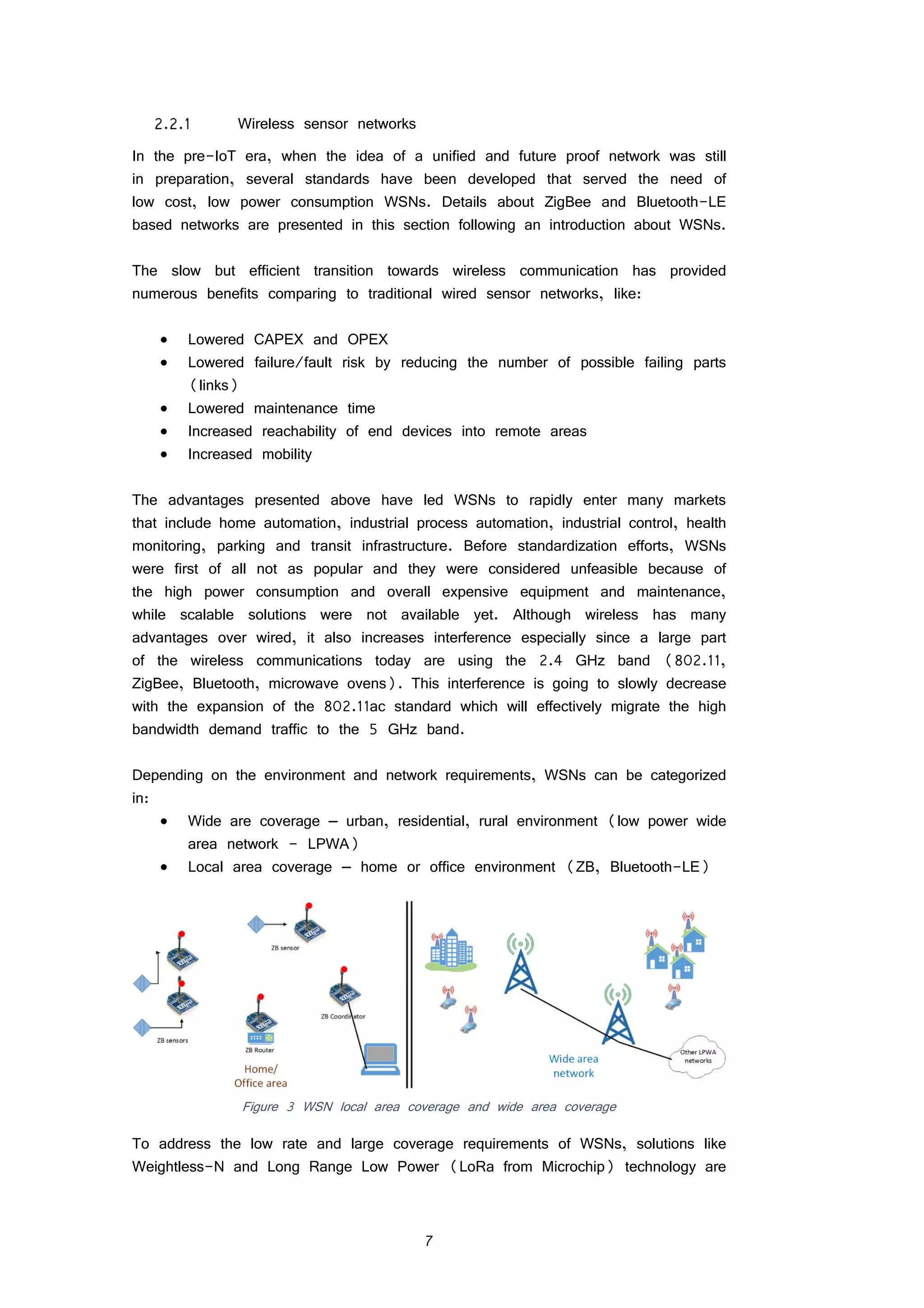
2.1 Sensor networks
The following sections regarding sensor networks and wireless networks are meant
to provide the reader with relevant information and theoretical aspects to the scope
of this project. In the first part, the reader is introduced to sensor networks and

13. 5
the connection with IoT devices, while the second part is dedicated to wireless
networks and specifically wireless sensor networks.
Sensor networks have shaped the way we perceive and influence the environment
to a certain degree of detail, offering a wide range of services and information.
Initially these types of networks were not standardized, but with the emerging IoT
and the expansion of sensor networks to health care, automotive, home automation,
security and many more sectors, the need for a global set of standards is growing.
As discussed above, wide coverage M2M devices are being deployed on mobile
networks, but solutions for offloading mobile data traffic are needed and wireless
networks optimized for low rate and low power provide a good solution.
Figure 1 Sensor node architecture
Sensors are much like the human senses and they respond to a physical change
(like temperature, light, movement) in the environment they monitor. This response
produces inside the sensor an electrical signal which is processed and sent through
a wired or wireless connection to the unit that is responsible of further conversion
and processing. Sensors were developed as a way to better understand the
surrounding environment. Nowadays we are surrounded by sensors and they can
be found in mobile phones, cars, houses, bikes, in most electrical devices and
more. In the figure below, the architecture of a sensor node, and a basic idea
about how the components interact, is represented.
Recent evolution in technology and the limitation of the current power grid has led
to the development of smart-grid technologies. This transition to a digital network
presents many advantages like two-way communication, self-monitoring capabilities
and a network topology with distributed generation unlike the existing one with
radial layout and centralized generating capacity. The sensor market is facing new
challenges and benefits from new opportunities with the development of such a
grid with its goals being to increase efficiency, reliability and security [6]. Real-
time sensing and processing of information is very costly in power requirements
and it’s an unfeasible solution for sensor networks containing a large number of
end devices. In order to achieve very low power consumption, such a network
must use elements and technologies capable of providing an efficient, long term
solution to this issue. Over the past decades, sensors have become much smaller,
energy efficient and less expensive, but even though the cost of the sensor has

14. 6
been greatly diminished, the cost to install them is way too high. In industrial
process automation the usual price for installing a wired sensor can be up to
$10,000 [7]. Because of this high cost, most sensors only transmit data to a
local controller in which case we cannot have an overall knowledge of a network
involving thousands of sensors. This led to the development of Wireless Sensor
Networks (WSN).
Figure 2 Sensor network architecture/star topology
This introduction to sensor networks was meant to provide the reader information
concerning the need that drove the development and rapid expansion of wireless
sensor networks and supporting protocols.
2.2 Wireless networks
This section is dedicated to understanding some of the wireless communication
technologies that facilitate the development of wide area WSNs and the impact
that global standardization of 4G/LTE for M2M devices has upon standards like
ZigBee and Bluetooth-LE and other proprietary LPWAN solutions like Sigfox and
Weightless.
The development of ALOHAnet in 1971 at the University of Hawaii, the first
wireless packet data network was an important step in further researching wireless
communication systems including 2G, 3G and WiFi (IEEE 802.11). The
development of smart devices capable of internet connectivity has led to an increase
in research done on possible solutions that fulfill the requirements of security,
scalability and performance of the IoT. Having this in mind, more traffic will be
offloaded from cellular networks to WiFi by 2016 [36].

15. 7
Wireless sensor networks
In the pre-IoT era, when the idea of a unified and future proof network was still
in preparation, several standards have been developed that served the need of
low cost, low power consumption WSNs. Details about ZigBee and Bluetooth-LE
based networks are presented in this section following an introduction about WSNs.
The slow but efficient transition towards wireless communication has provided
numerous benefits comparing to traditional wired sensor networks, like:
 Lowered CAPEX and OPEX
 Lowered failure/fault risk by reducing the number of possible failing parts
(links)
 Lowered maintenance time
 Increased reachability of end devices into remote areas
 Increased mobility
The advantages presented above have led WSNs to rapidly enter many markets
that include home automation, industrial process automation, industrial control, health
monitoring, parking and transit infrastructure. Before standardization efforts, WSNs
were first of all not as popular and they were considered unfeasible because of
the high power consumption and overall expensive equipment and maintenance,
while scalable solutions were not available yet. Although wireless has many
advantages over wired, it also increases interference especially since a large part
of the wireless communications today are using the 2.4 GHz band (802.11,
ZigBee, Bluetooth, microwave ovens). This interference is going to slowly decrease
with the expansion of the 802.11ac standard which will effectively migrate the high
bandwidth demand traffic to the 5 GHz band.
Depending on the environment and network requirements, WSNs can be categorized
in:
 Wide are coverage – urban, residential, rural environment (low power wide
area network - LPWA)
 Local area coverage – home or office environment (ZB, Bluetooth-LE)
Figure 3 WSN local area coverage and wide area coverage
To address the low rate and large coverage requirements of WSNs, solutions like
Weightless-N and Long Range Low Power (LoRa from Microchip) technology are

16. 8
being developed and implemented. These types of wireless networks fall into the
category of LPWA networks which will play an important role in the development
of IoT devices. On a smaller scale, e.g. home automation system, coverage
requirements may be much smaller and solutions like ZigBee and Bluetooth-LE
are available in a local area network. Proprietary solutions which include gateways,
sensor nodes, routers and cloud storage are available for both technologies. For
the scope of this project, the communication protocol ZigBee was chosen to provide
coverage and data transfer in the implemented WSN. The justification behind this
solution stands in the large availability of compatible products and support information
as well as the low price in comparison with similar products. More details about
the components used will be provided in the implementation chapter.
The continuous price reduction of electronics over the years alongside the deep
market penetration level of electronic products and affordable personal computers,
has benefitted the development of a new type of computational board with personal
computer capabilities available to everyone. The idea behind these boards was to
devise a small and cheap computer that was meant to inspire children and
consequently set in motion the new generation of consumer electronics. The latest
advances in technology have brought forth interactive development boards like
Arduino and Raspberry Pi for high computational power and together with
communication protocols like ZB and Bluetooth-LE, the basic requirements for a
local, low cost and low power consumption WSN are met.
The increased efforts for providing scalable solutions and standards to meet the
requirements for deploying IoT devices on a large scale has led to an increase
in global competitiveness and consequently an improved quality of products and
service for the customer. Another driving factor that enabled this rapid development
was the huge profit opportunities presented by the unsaturated global market. All
things considered, WSNs are contributing to the increased sensing accuracy and
lowered control granularity of our surroundings, at the same time increasing the
efficiency of risk prevention methods and providing an overall improved quality of
life.
ZigBee
The ZigBee (ZB) communication protocol has proven to be a reliable and mature
network. Its highest usage today is in application development. Considering the
high market penetration of M2M devices by the year 2020, the ZB protocol will
play an important role in providing solutions in a limited range environment like an
office or home. The topology of the network can be observed in figure 4.

17. 9
Figure 4 ZigBee network topology
In the late ‘90s, many engineers began to think whether Wi-Fi and Bluetooth
were enough for the ever growing wireless in-home network control and monitoring
applications. Because of this rapid expansion and the inability of the existing
technologies to be suitable for future applications, a new type of network was
needed and the ZigBee communication protocol began to be standardized by the
IEEE right before the end of the century. The IEEE 802.15.4 standard, which
specifies the physical layer and the MAC sub-layer for LR-WPANs (Low Rate
Wireless Personal Area Network), was finished in 2003 and has experienced a
large growth over the years. There are several extensions to IEEE 802.15.4 and
one of them is ZigBee (ZB). The ZB protocol is shown in figure 5.
Figure 5 ZigBee protocol stack
ZB represents one of the standard-based wireless technologies developed to
address the needs of the low cost and low power wireless sensor and control
networks. It can be implemented almost anywhere, thus the opportunity of growth
is endless. What makes ZigBee so useful in the development of WPANs is the
low consumption inherited from 802.15.4. The end devices are capable of sleeping

18. 10
up to 99% of the time and the tasks needed to send and receive information use
a small part of the devices’ energy, increasing battery life to years. Besides being
low cost and low power, ZB is flexible, allowing users to easily upgrade their
network in terms of security and efficiency. A few services that differentiate the
ZigBee protocol are:
 Association and authentication
 Routing protocol – an ad-hoc protocol designed for data routing and
forwarding: AODV [4]
Because the 2.4 GHz ISM band is also in use by microwave ovens, cordless
telephones, Bluetooth devices and the 802.11b/g standards, ZB may suffer from
heavy interference which is produced mostly because of the overlapping adjacent
frequency channels and heavy usage of this band, as only 3 non-overlapping
channels are offered out of the 16 on the 2.4 GHz band. To combat this
interference, the 802.15.4 protocol makes use of two techniques:
 CSMA-CA (Carrier Sense Multiple Access-Collision Avoidance) – maximum
16 TS
 GTS (Guaranteed Time Slots) – not suited for large number of devices
Another important aspect to consider when designing a WSN is reliability, so the
integrity of the information sent is verified through the use of ACK and NACK
messages between the transmitter and receiver. These kinds of packets are one
of the two most relevant types of packets that the ZigBee network transmits, the
others being data packets [4]. A few features of the ZigBee standard are presented
in table 1 [65].
Although the ZigBee protocol is using the same IEEE 802.15.4 RF protocol the
addressing and message delivery systems are different because of the added mesh
networking capabilities. There are two types of addressing: extended and network.
The extended address is a static 64-bit address which is guaranteed to be unique
and it is used to add robustness. The network address is a unique 16-bit address
which is assigned by the coordinator to a new node in the network. The extended
address is required in sending a message to the network while the network address
is not. Just like 802.15.4, broadcast and unicast messages are supported in
ZigBee.
Table 1 ZigBee network characteristics [65]
Attribute Characteristics ZigBee
Range
As designed 10-100 m
Special kit or outdoors Up to 400 m
Data
Rate
20-250 Kbps
Network
Network join time 30 ms
Sleeping slave changing to active 30 ms

19. 11
New slave enumeration 15 ms
Active slave channel access 15 ms
Power Profile Up to 6 years
Protocol Stack 32 KB
Operating Frequency
868 and 915 MHz and 2.4
GHz ISM
Network Topology
ad-hoc; star; mesh (full mesh
networking support); hybrid
Number of Devices per Network Up to 65,536 network nodes
Security
128 bit AES, appl. layer
definable (standard algorithms)
In contrast with traditional cellular technologies which rely on a star network
topology, ZigBee networks can benefit from a mesh topology with self-healing and
self-organizing properties to better scale in an IoT scenario. Increasing the number
of devices in a ZB network increases complexity and a very large number of
devices in the same network becomes unfeasible for the low cost and low power
characteristics of an IoT network. Given a small number of devices, for example
in a home-automation system or office area, ZigBee can be deployed in a star
topology.
Bluetooth-LE
Bluetooth (BLT) technology is a wireless communication system which was
developed to overcome the wiring problem which arose from the need to connect
different types of devices like mobile phones, headsets, and power banks, other
media devices and medical equipment. Some of the requirements for BLT technology
are:
 Low power consumption
 Low price
 Small dimensions
Having these attractive requirements, the technology was quickly adopted in 1998
by major manufacturers like Ericsson, Intel, IBM and Nokia who provided the
necessary and diverse market support needed. Given its advantages in power
consumption and price, the technology has quickly evolved into a global standard
and is now found in most mobile phones, laptops, tablets and many electrical
devices including bike locks. Similar to its competing technologies (IEEE 802.11,
ZigBee and UWB (Ultra-Wideband)), Bluetooth is operating in the ISM spectrum
of 2.4 GHz, but in addition to data communication, it is designed to support voice
as well. The coverage of this technology is applications specific and vendors may
tune their products based on need, although the specifications dictate that it should
operate over a minimum of 10 meters depending on device class. The latest
specifications (Bluetooth 3.0 and 4.0) in terms of speed permit BLT devices to
exchange data at up to 25 Mbps, which is a great improvement comparing with

20. 12
earlier versions (Bluetooth 1.0) which had 1 Mbps, although most IoT devices
and applications require low data rates for the specific purpose of saving energy.
Although it was designed to replace cables, Bluetooth has evolved into a competing
technology for the emerging IoT with its ability of creating small radio LANs called
piconets or scatternets (a network of piconets). The latest update, Bluetooth-LE
(low energy) features ultra-low power consumption so devices can run on for
years on standard batteries as well as low costs of implementation and maintenance.
Unlike ZB which was defined on an existing protocol stack, the IEEE 802.15.4,
BLE was developed taking into account low power consumption on every level
(peak, average and idle mode) [41]. The BLE architecture can be seen in figure
6, below.
Figure 6 Bluetooth LE stack
It uses the ATT (Attribute protocol) to define the data transfer on a server-client
basis. Its low complexity directly influences the power consumption of the system.
The Generic Attribute Profile (GATT) is built on top of this protocol and it’s
responsible with providing a framework for the data transported and stored by the
ATT by defining two roles: server and client. ATT and GATT are crucial in a
BLE device since they are responsible for discovering services. The GATT
architecture provides accessible support for creating and implementing new profiles,
which facilitate the growth of embedded devices with compatible applications [41].
The low power consumption character of BLE in idle mode is given at the link
layer which is also responsible for the reliable transfer of information from point to
multipoint. Considering the re-designed PHY layer of BLE in contrast with previous
versions, two modes of operation were defined: single and dual mode. The
advantages of dual mode consist in compatibility between BLE devices and earlier
version devices, while single mode is the preferred solution in battery powered
accessories because of lower power consumption. At the link layer, power can be
conserved in a slave device by tuning the connSlaveLatency parameter which

21. 13
represents the “number of consecutive connection events during which the slave
is not required to listen to the master” and can have integer values between 0
and 499. A connection event in this case is a non-overlapping time unit in a
physical channel after a connection between a master and a slave has been
established [41, 43].
One very important feature of the IoT is scalability considering the billions of
devices that will flood almost every environment during the next 5 to 10 years.
Bluetooth classic has the capability to create small LANs in order to exchange
various data like photos or videos, but the address space of 3 bits only allows
for maximum 8 devices in the same network. [42] Although this represents a
great feature for very small areas, it doesn’t provide a scalable solution for large
networks involving M2M devices with low power consumption. BLE instead has a
32-bit address space which means that, theoretically, the network size can be
the same as for IPv4, more than 4 billion. However, there are limitations to this
number given by the type of communication between master and slave and certain
parameters, like BER and connInterval. This parameter represents the “time between
the start of two consecutive connection events” [43]. The values that this parameter
can take are a multiple of 1.25 ms between 7.5 ms and 4 s.
Considering the evolution of Bluetooth, which started out as a wireless
communication technology to replace cables, it has taken great steps into providing
a reliable and cost effective solution for wireless communication systems on a
global scale. The small hardware dimensions as well as the power efficiency have
made this into a most wanted technology in most smart phones, laptops and many
other wireless capable devices powered by battery. The latest update, BLE, is
meant to extend its usage to IoT devices by providing ultra-low power consumption
in end devices and increased network size for scalability purposes. Although the
Bluetooth SIG has made great efforts to provide this solution, BLE is still facing
some problems that make it less appealing for IoT applications:
 The operating frequency of BLE is 2.4 GHz in the ISM unlicensed spectrum.
The already high interference level at this frequency will only get worse
by introducing millions of new devices resulting in much lower reliability.
 Although the PHY layer data rate is 1 Mbps, testing done in this [43]
article has shown that the maximum application layer throughput is 58.48
kbps due to implementation constraints and processing delays. This value
may be enough for some IoT applications, but it’s not a solution in case
of higher data transfer applications.
 Unlike other technologies working in sub-GHz spectrum, the coverage of
BLE is limited and the 2.4 GHz band is not the most suited for wall
penetration (e.g. basement) or in rainy situations. Creating scatternets
may prove as a solution to extending coverage, although this creates high
network complexity.

22. 14
2.3 Cellular networks
This section is dedicated to assessing the possible solutions for the IoT provided
by cellular technologies. Currently deployed cellular technologies like 2G, 3G and
4G/LTE were not designed to handle billions of devices working on
Mobile networks continue to expand at an alarming rate and optimization techniques
are constantly used to provide a seamless experience for the users. Today, the
majority of mobile data traffic (~80%) is transferred indoors. This presents a big
challenge for network operators to provide solutions for the constant demand for
faster and better quality data. Standardization efforts from the 3GPP group are
also increasing and it is imperative to plan a few steps ahead considering the
fast expansion. As discussed earlier in the introduction, the impact of the Internet
of Things on the mobile data traffic is not something to ignore. Cisco predicts
that by 2020 more than 20 billion M2M devices (home automation, smart
metering, maintenance, healthcare, security, transport, automotive and many more)
will have internet connectivity comparing to 495 million in 2014 [36]. Although
only about 200 million will have mobile network connectivity according to a white
paper from Nokia [50], representing a 26% increase in CAGR.
Another category with high growth potential among internet connectable gadgets is
represented by wearable devices like smart watches, health monitors, navigation
systems and more. These devices can either connect directly on the network or
through a mobile device (via Wi-Fi or Bluetooth). It is estimated by Cisco that
by 2019 the wearable devices (e.g. smart watches, health care devices) will
reach approximately 578 million globally, having a CAGR of 40% [36]. In figure
7 a visual representation of CAGR increase between 2014 and 2019 is shown.
Figure 7 Global mobile data traffic, 2014-2019 [34]
In the following paragraphs, a few details about mobile networks history are
presented followed by a more detailed view on the relevant technologies for this
project.

23. 15
As opposed to traditional wired networks in which a connection between two users
is established through a physical link, mobile networks are characterized by the
use of wireless communication technologies to deploy services to users. The cellular
concept of mobile networks was defined first in 1947 [32], a radical idea at that
time when most of the research was about providing radio coverage on an area
as large as possible from one base station (BS). This was in contradiction with
the cellular concept which proposed limiting the signal from a BS to a specified
area in order to reuse the same frequencies in neighboring cells, which had their
own transceiver. Such a system permitted the subscription of many more users in
a region, but this only became feasible in the 1980s when the advances in
technology brought forth electronic switches, integrated circuits and handover
techniques [32, 18]. Another factor that impeded the earlier deployment of cellular
networks were the lack of standardization efforts.
The first generation of mobile networks was commercially deployed in the 1980s
and it was solely based on classic circuit switching (CS). This method involved
switching analogue signals in a switching center with the help of a matrix which
mapped all the possible source and destination paths. Communication was possible
both ways once a physical connection was established between the two end points
(hosts) [18, chapter 1].
Following this introduction, the following sections explore the different characteristics
of the relevant generations of mobile networks.
2G
The following subsection has the scope of introducing the reader to the most
important elements that make up the second generation network. GSM represents
the foundation for all future cellular networks.
2G (GSM) represents the second generation wireless telephone technology which
was a great improvement in 1991 since it introduced digital communication over
the traditional analogue and more efficient usage of spectrum. Being the first
commercially deployed wireless digital communication technology, GSM has been
implemented in most of the countries around the globe given its increased
accessibility over the years. This had a direct effect on the availability of the
system which led all further upgrades (GPRS, EDGE, UMTS, HSPA and LTE)
to provide compatibility with GSM in the absence of a better technology. Other
reasons were cost and time required to deploy a new infrastructure. In figure 8
the GSM network architecture is presented.

24. 16
Figure 8 GSM network architecture
Some of the most important functions performed by GSM’s network elements are:
channel allocation/release, handover management, timing advance
The GSM standard only allows 14.4 kbps over the traffic channel (user data
channel) which can be used to send digitized voice signal or circuit-switched data
services. GSM only allowed a circuit switched connection over the network and
thus billing for data was done per minute connected. [18] Despite the voice
oriented design of 2G, several upgrades have been added to the network to
facilitate the transfer of more data and faster over the same infrastructure. One
major update, that would eventually become the focus of future mobile networks,
was the introduction of data communication, namely the PS network. On GSM,
SMSs are sent through the signalling channels, but from GPRS onwards, the SMS
is treated as data and it is being conveyed on the traffic channel.
By the year 2000, mobile phone users were already experiencing the data friendly
GPRS (General Packet Radio Service). With this release, data services
experienced a large growth and data rates of up to 70 kbps were realistic. This
upgrade was possible due to the improved radio quality and dedicated TS for
data. The biggest differences in the new architecture were the addition of a packet
switched core network to deal with all the data traffic available and a PCU (Packet
Control Unit) to be installed on all BSC to provide a physical and logical interface
for data traffic. Unlike GSM, billing for data connection was done per traffic volume.
These architecture differences can be seen in figure 9. Alongside a packet control
unit, the PS network also contains a GGSN (Gateway GPRS Support Node)
which routes packets and interfaces with external networks and a SGSN (Serving
GPRS Support Node) which is responsible for registration, authentication, mobility
management and billing information. Soon after, in 2003, EDGE (or 2.75G) was
being deployed on GSM infrastructure and was introduced as the “high-speed”
version of GPRS. This release, almost as powerful as 3G, was capable of
delivering realistic data rates of up to 200 kbps by using a new modulation
format, new coding schemes and incremental redundancy.

25. 17
Figure 9 GPRS Architecture
The vast accessibility of GSM around the globe has ensured its long existence,
although a full transition to the PS network is desired because of the huge costs
of maintaining two networks at the same time. The solution for an only PS network
has been specified starting with release 7 from 3GPP [36]. Fallback to the CS
network is possible in case of PS network failure though the CS Fallback
procedures, also specified by 3GPP.
An analysis on the amount of users/mobile network performed by Cisco in 2014
shows that the majority of mobile devices, 62%, are using 2G for connectivity. It
is estimated that by 2017 GSM will no longer be the majority holder of mobile
connections, dropping down to only 38% and by 2019 to 22% [36]. An evaluation
of technology adoption for M2M devices in 2014 was performed by EMEA and
the results showed that 2G is still the preferred technology in automotive industry,
transportation, energy and security. The primary reason behind favoring 2G networks
for M2M devices is the price to embed 2G connectivity onto devices, followed by
worldwide availability of the network [37].
In the 2G section, a few important details were covered about the mobile network,
ending with a short evaluation on the impact of 2G in mobile networks today, as
well as the impact and relation with M2M devices.
3G
A few details about the involvement of 3G in the IoT are discussed in this section
and also the how it relates to the current project. The following part will be
dedicated to detailing a few characteristics of 3G networks and what were the
driving factors into developing this network.
The 3G network represents a transition network from a few points of view. On
one side, it’s meant to provide a smooth evolution to an only PS network. As
discussed before, maintaining 2 networks (CS and PS) at the same time can
be very costly and inefficient. From another point of view, the transition of M2M

26. 18
devices from 2G to LTE networks is also happening gradually through the 3G. By
2016, a report from Sierra Wireless predicts that most of the technological sectors
(including automotive, transportation, energy and security) will provide support for
3G connectivity. For the purpose of this project, this is the main network responsible
with internet connectivity.
The 3G network today represents a transition network between the old circuit
switched and the future only packet switched networks. The 2nd
generation mobile
networks limitations, like “the timeslot nature of a 200 kHz narrowband transmission
channel and long transmission delays” [18, page 116], did not permit a further
upgrade and so, by the end of the millennia, the standardization of UMTS (3G)
was finished and it presented capabilities far beyond that of the previous generation.
The most important requirements taken into consideration for this new system were
the increase in bandwidth, flexibility and quality (QoS).
Figure 10 UMTS network architecture
Considering the architecture of the 3G network in figure 10, besides the same
core network a few major changes can be observed in the radio access network.
For example the BS is now called Node-B but maintains the same functions as
a BS. New interfaces are specified (Iu, Iur, Iub and Uu) for communication
between different network elements. In the Radio Network Subsystem (RNC) the
BSC is replaced with Radio Network Controller (RNC) which control the Node
Bs.
Although this is a new generation of mobile networks, UMTS was not built from
zero and initially reuses a lot of GSM and GPRS with the exception of the radio
access network (UTRAN), which was completely new. The new radio interface
uses 5 MHz frequency channels with bit rates that reach up to 384 kbps with
the new WCDMA multiplexing scheme, which supports more users compared to
TDMA. In this new coding scheme, everyone is transmitting at the same frequency
and at the same time, resulting in a high spectral efficiency. Even though this is

27. 19
very efficient usage of spectrum (frequency reuse factor = 1), the overall capacity
and coverage of the network decreases with the increase in connected users to
the same cell [18, chapter 3]. EDGE Evolution was developed after the release
of 3G and it was designed to improve coverage for HSPA (High Speed Packet
Access). Maximum throughout achieved can be up to 1.3 Mbps in downlink [22].
As discussed previously in the 2G section, currently 62% of devices use GSM for
connectivity, but in the near future this will drop to 38% in favour of 3G initially
with an emphasis on 4G later on. By 2017, 45% of devices will function on 3G,
although the growth will rapidly stabilize and even fall by 2019 to 44% [36].
LTE/4G
This sub-section presents on overview of the LTE (Long Term Evolution) standard
as well as 4G together with a few details about the implications and benefits of
M2M devices in relation to LTE-M.
The advances in cellular networks from lower-generation networks (2G) to higher-
generation networks (3G, 3.5G and 4G/LTE) are partly due to the increasing
computing capabilities of end devices which demand higher BW (bandwidth).
Therefore, the adoption of 4G and its overall deployment is rapidly increasing. The
fastest adoption rate is observed in the USA with 19%, while Europe is only at
2% in 2014 [37]. Currently only 6% of devices are using 4G, but by 2019 Cisco
estimates an increase to 26%. At the same time, the amount of data generated
by 4G networks by 2019 will represent 60% of the total [36].
The evolution towards an exclusive PS network is realized through a series of
supporting technologies developed around the 4G standard. Solutions like IMS VoIP
(Internet Media Services Voice over IP) and SMS over IP are fully specified by
3GPP in release 7 (3rd
Generation Partnership Project) in the LTE standard
[34]. Initially voice information was delivered through the CS network which is
presents in both 2G and 3G. 4G was designed to be the mobile network of the
future and along with it the transition from CS networks to PS network is complete,
although as discussed above, fall back solutions to former CS services are
available. Through a series of new network elements, the 4th
generation network
manages to maintain only one network. The overall simplicity of the packet-oriented
of network is due to a few changes in how it is functioning and handling data.
For a start, the new eNode-B (evolved Node-B) has completely took over the
radio related functionalities of the former RNC, like resource allocation, scheduling,
re-transmission and mobility management. The PS and CS networks were combined
into EPC (Evolved Packet Core) which efficiently handles incoming data by
separating user and control planes. The control is now handled by the MME
(Mobility Management Entity), which is responsible with authentication, security,
mobility management as well as subscription. The SGW (Serving Gateway) handles
all user switching and data forwarding as well as access to external networks
through the PDN-GW (Packet Data Network Gateway) [18, chapter 4].

28. 20
Figure 11 LTE network architecture
An important aspect of the 4th
generation mobile network that is directly influencing
the IoT is BW allocation. As discussed above, more than 3 billion IoT devices
are expected to have data connectivity and out of those, Cisco predicts that only
13% will have connection through 4G in 2019 [36]. On top of this, the wearable
devices market is also growing considerably and will present an impact on the
amount of mobile traffic. The justification of adopting M2M devices on the 4G
network is given by the significant revenue opportunities for mobile operators as
well as the general desire to migrate 2G traffic to 4G. M2M devices designed for
4G should also be produces at the lowest cost in order to be cost effective with
GSM/GPRS devices [39].
Starting with release 12 [39], 3GPP has begun specifying a new category of
M2M devices that would be feasible and compatible with the existing infrastructure.
These devices are specified under the LTE-MTC (LTE-Machine Type
Communication), details of which shown in the sub-section below.
The cellular networks presented above represent the existing technologies that were
developed for the specific purpose of standardized global mobile communication.
The second generation 2G network, the first globally deployed cellular network
which provided a leap forward from analogue transmission, together with the
following upgrades 3G and 4G have focused primarily on providing efficient and
scalable solutions for voice and data communication. Considering the requirements
of IoT devices and networks, these existing solutions are not designed to integrate
billions of devices with completely different types of transmissions and capabilities.
The remaining sections of this chapter are focused on understanding the implications
that IoT brings and what is required in the development of such a communication
system.
2.3.3.1. LTE-M
The mobile internet trend has been to constantly increase capacity for high BW
consumption applications and broadband services leading to very high data rates
in LTE and 4G networks. The M2M devices are designed for low BW consumption

29. 21
and so, wide area M2M connectivity requires new standardization efforts to the
current technologies. Some of the key requirements of M2M devices for LTE are
[38, 39]:
 Wide service spectrum – diversity in types of services, availability and
BW.
 Low cost connected devices
 Long battery life
 Coverage enhancements – placement of devices in low or no signal
areas
 Support data rates at least equivalent to EGPRS
 Ensure good radio frequency coexistence with legacy LTE radio interface
and networks
Beside the requirements presented above, considerations for addressing (IPv6 is
recommended), signaling and roaming need to be investigated. The existing LTE
network architecture is sufficient for the time being, but the fast growing number
of M2M devices and the rapid adoption pace towards 4G requires new network
elements to handle the new features and the many different types of services
[38]. Design consideration of M2M devices following a low cost scenario include:
 1 Rx antenna
 Downlink and uplink maximum TBS (Transport Block Size) size of
1000 bits – means that peak data rates are reduced to 1 Mbps
in downlink/uplink (DL/UL) [38]
 Reduced downlink channel BW of 1.4 MHz for data channel in
baseband while uplink channel BW and downlink and uplink RF
remains the same as for normal LTE UE [39]
 Optional: half duplex FDD devices will be supported for additional
cost savings
Following de design considerations mentioned above, a few potential techniques for
improving LTE M2M device coverage on the physical channel are shown in table
2.
Table 2 Potential coverage enhancements techniques on physical channels [62]
Technique PUCCH PRACH PUSCH EPDCCH PBCH PDSCH
PSS/
SSS
Repetition/subframe
bundling
X X X X X X
PSD Boosting X X X X X X X
Relaxed Requirement X X
Overhead reduction X
HARQ retransmission X X
Multi-subframe channel
estimation
X X X X X

30. 22
Multiple decoding
attempts
X
Increased reference
signal density
X X
Taking into consideration the requirements mentioned above, the LTE-M standard
is developed to support long battery life of 10+ years for end-devices in order to
follow the most cost effective plan. In release 12 [39] a power saving mode
(PSM) is introduced which significantly improves battery life of end devices. This
sleeping mechanism allows the device to stay registered with the network in order
to reduce signaling and consequently reduce power consumption. A similar sleeping
mode was discussed in the ZigBee section, although in contrast with the ZB
sleeping cycle, a M2M device remains in PSM until it is queued to perform a
network procedure. In release 13 from 3GPP, this feature is improved even further
e.g. increasing DRX (Discontinuous Reception) cycle form 2.56 seconds to 2
minutes results in a battery-life increase from 13 months to 111 months. In table
3 are shown different features available with the current and future 3GPP releases.
Table 3 LTE features for M2M services [62]
LTE Release Feature
Rel-11 (2012)
 UE power preference indication
 RAN overload control
Rel-12 (2014)
 Low-cost UE category (Cat-0)
 Power saving mode for UE
 UE assistance information for eNB parameter tuning.
Rel-13 (2016)
 Low-cost UE category
 Coverage enhancement
 Power saving enhancement
Although LTE-M has been specified by 3GPP, the high costs of deploying end
devices that integrate into the LTE network is not feasible at the moment. As
discussed in the section above, only 13% of total M2M connections worldwide will
be supported by LTE-M [36] by 2020, while more than 50% will be supported
by 2G and 3G.
2.4 Low Power Wide Area Networks
The numerous standardization efforts today that are focused on IoT devices and
related communication protocols are looking to provide solutions for local or regional
area networks, solutions which can effectively offload the M2M traffic from the

31. 23
global 4G network. In a white paper from Cisco [36], the migration of wide area
M2M devices from 2G to 3G and ultimately to 4G is taking a fast pace and by
2019, 4G M2M devices will reach 13% of the total M2M connections, while 3G
will hold 35% and 2G only 23%. By that time, LPWA networks will also play an
important role in transporting the large amount of M2M traffic, which will represent
29% of the total connections.
Figure 12 LPWA network deployment scenarios
Some of the requirements for LPWA networks include:
 Low throughput
 Low power
 Wide area coverage
 Scalable solution
 Low cost
The sub-GHz spectrum provides high signal propagation while maintaining a low
cost for end device equipment. This enables radio waves to provide connectivity
in basements or behind thick concrete walls. The wide area coverage of these
low power networks is a driving factor for large scale deployment in all types of
environments as shown in figure 12. The cloud based controller is responsible with
keeping track of all network elements and traffic handling. Considering this use
case application and how data will be managed in the IoT, a possible architecture
is considered in the next subsection.
IoT architecture
Following the big success of cellular networks in terms of scalability, coverage and
low complexity, the technologies that are meant to support the IoT are being
developed having the same topology in mind. The major difference in an IoT
network is that devices are meant to communicate between themselves without the

32. 24
need for human interaction. This type of communication (M2M) has many
advantages over conventional types, but at the same time it requires new network
architecture, protocols and capabilities that are designed to handle the amount of
connections. The end devices in an IoT network, unlike the UEs in current cellular
technologies, are built in with much lower power consumption and less complexity
which adds up to the overall lower cost.
Figure 13 IoT Architecture
In figure 13, a possible IoT Architecture is proposed. In this scenario, all 3 types
of communication can be observed. A device-to-device (D2D) type of
communication can be seen as a peer-to-peer (P2P) architecture where data is
exchanged between peers without having to distribute it through a central
node/server. In contrast with a client-server model, in a P2P architecture the total
bandwidth of the network increases as the number of peers increase. A D2D
architecture may also function on a client-server model and it follows a
request/response type of messaging exchange. This synchronous data interaction
between devices means that one device is making a request and has to wait for
a response. The client-server congestion problem will be discussed further in the
scalability section below. In a different type of communication where a broker is
needed to route the information further, the messaging pattern follows a
publish/subscribe model. In this case, the publisher doesn’t know about the
existence of a subscriber and vice versa. These messaging patterns are shown in
figure 14.

33. 25
Figure 14 Messaging pattern
Weightless
The last two subsections of this chapter focus on cellular networks which were
designed specifically to meet the requirements imposed by the IoT. Some of the
most important requirements, as mentioned also in the first chapter, are:
 Ultra-low power consumption (battery powered or battery-less devices
or sensors)
 Low to moderate data-rates
 Highly scalable design (reasonable coverage)
 Low complexity of devices (which leads to overall lower costs of
implementation and maintenance)
 Support for a very large number of connected devices
 Reliable and secure devices and communication technologies
 Delay tolerant
Looking at the requirements above, it can be easily concluded that the mobile
communication networks were not designed to support the IoT, although solutions
like LTE-M discussed above can prove as a feasible solution for a certain
percentage of the total amount of connected devices. At the same time, M2M
devices compatible with 2G and 3G are already being deployed, but without
extensive network improvements in the future, these mobile networks will not be
able to support the huge number of connected devices or the amount of traffic
and signaling. Moreover, subscription and device costs are much higher in a mobile
network like 2G, 3G and 4G/LTE. Unlike these mobile networks which provide
solutions for human-to-machine-to-human type interactions, the cellular networks
presented here are designed to address the need for low cost, low power and
high propagation characteristics of M2M type communications. The end devices in
these cellular networks are battery powered or battery-less gadgets which need to
perform well established tasks in environments where sub-GHz spectrum has much

34. 26
higher propagation (behind thick walls, basements, sewers) as opposed to current
cellular technologies which operate on higher frequencies, unsuitable for these tasks
in these environments.
The Weightless open standards which are designed as a cellular low power wide
area network operate on sub-GHz license free spectrum. Competing technologies
like ZigBee, Bluetooth-LE and Wi-Fi which also operate on unlicensed spectrum
but on higher frequencies (2.4 GHz) offer cheap endpoints as well, but the
coverage of these solutions is much smaller and can only account for short-range
applications. The coverage required in sectors like automotive, healthcare and asset
tracking is much larger than these technologies can provide. Depending on the
application and the environment, Weightless has defined 3 standards to provide
support in all the sectors that will benefit from the IoT. The table below shows
the differences between these standards.
Table 4 Weightless open standards [44]
Weightless-N Weightless-P Weightless-W
Directionality 1-way 2-way 2-way
Feature set Simple Full Extensive
Range 5km+ 2km+ 5km+
Battery life 10 years 3-8 years 3-5 years
Terminal cost Very low Low Low-medium
Network cost Very low Medium Medium
The high propagation characteristic of Weightless-N is achieved by operating on
sub-GHz spectrum, using ultra narrow band (UNB) and software defined radio
technology. This technology offers the best tradeoff between range and transmission
time. Transmission on narrow frequency bands is realized by digitally modulating
the signal with a differential binary phase shift keying (DBPSK) scheme and
interference mitigation is accomplished by using a frequency hopping algorithm. The
UNB technology behind this standard is provided by Nwave, a leading provider of
network solutions for the IoT, both hardware and software. The problem of multiple
Weightless networks operated by different companies in the same area is solved
by using a centralized database to determine in which network the terminal is
registered for decoding and routing purposes. At the same time the advanced de-
modulation techniques make it possible for Weightless to co-exist with other radio
technologies working within the ISM bands, thus avoiding collisions and capacity
problems [44]. Database querying is done by base stations. The star architecture
allows up to 1,000,000 nodes to connect to one base station [45]. The network
architecture for a Weightless based communication network is shown in figure 15,
below.

35. 27
Figure 15 Weightless network architecture
The Weightless-W standard was the first of these standards to be released and
its most important feature is the usage of TV white space spectrum. This unlicensed
white space represents the unused TV channels which account for approximately
150 MHz in most locations around the world [47]. This means that the TV
spectrum will be used by both licensed and unlicensed users which will unavoidably
create interference. In order to maximize the spectrum usage and avoid interfering
with TV channels, out-of-band emissions have to be minimized and depending on
application, modulation schemes like DBPSK, SCM (Single Carrier Modulation)
and 16-QAM are used. Other methods of interference mitigation used are frequency
hopping, scheduling and spreading [46, 47]. This technique also represents a key
factor in designing these networks because it is the only way to achieve long
range with low power at the cost of throughput. Spreading factors from 1 to 1024
can be used based on the Weightless specification. In contrast with Weightless-
N, designed for applications that require very low data rates with 1-way
communication, data rates for end devices operating on Weightless-W are between
1 kbps and up to 10 Mbps with variable packet size depending on application and
link budget [46]. Weightless-W provides very flexible packet sizes from 10 bytes
with no upper limit and a very low overhead size of less than 20% in packets
as small as 50 bytes [47].
An important factor to take into consideration about Weightless is that it’s an open
global standard, leaving the user a lot of room for customization and future
innovation at a much lower cost than a mobile network.
Sigfox
One of the major competitors to Weightless is Sigfox, a cellular network designed
to address the specific need of very low throughput applications that are part of
the IoT. Similar to mobile networks, Sigfox is also an operated network in which

36. 28
deployed transceivers (base stations) provide the cellular connectivity to end user
devices. Device transmission is handled by the integrated Sigfox modems in M2M
devices designed to work with the Sigfox network. In figure 16, an M2M device
with an integrated Sigfox modem is regularly transmitting information. The base
station handles the data and routes it to the Sigfox servers which verify data
integrity. Ultimately the information from the servers is received through an API
designed to read the messages from the M2M device.
Figure 16 Sigfox use case
Being an operated network, users only need to purchase the Sigfox compatible
end devices which include specific management applications and APIs. Like the
Weightless-N standard, Sigfox uses patented UNB radio technology for connectivity
and transmission. The communication spectrum is provided by the ISM bands which
further lower the price for maintaining such a network. Sigfox is a frequency
independent network which means that it can comply with any ISM spectrum
depending on location and even with licensed frequencies and white spaces. The
UNB based M2M devices have “outstanding sensitivity” resulting in massive cost
savings allowing cheap subscriptions. Unlike Weightless, Sigfox is a proprietary
network and doesn’t provide much flexibility in terms of adaptability to the rapidly
expanding IoT trend.
Sigfox is differentiated from other competitive technologies by using ultra-low data
rates of 100 b/s [48]. This is advantageous in applications that require very low
throughput and seldom transmissions of data. At the same time, power consumption
is very low allowing end devices to operate up to 20 years with 3 transmissions
per day on a 2.5 Ah battery [48]. Having a very low and fixed data rate, Sigfox
doesn’t present much flexibility when it comes to the large number of different
applications that an IoT network can provide. LPWAN solutions that provide Adaptive
Data Rate (ADR) scale much better in terms of applicability, like Weightless and
Actility. Another downside for Sigfox in contrast with existing solutions is the
proprietary standard which doesn’t allow much flexibility in innovation and slows
down development.

37. 29
The Sigfox modems provided by the company are easily integrated in devices
destined for M2M wireless communication. The modems are based on standard
hardware components and have installed the Sigfox protocol stack. Reading Sigfox
messages is done through a web application that allows the user to register
HTTPS addresses of a proprietary IT system with the Sigfox servers. The messages
are then forwarded to the specified HTTPS address [48]. The web application
provides an overview of the network with all connected devices as well as power
status and connectivity issues alongside other relevant data, making the system
easy to access, configure and maintain.
Taking into account the very low power consumption and low throughput, the
network can be characterized as follows [48]:
 up to 140 messages/device/day
 payload size of 12 bytes/message
 data rate of 100 b/s
 range:
o rural – between 30 and 50 km
o urban – between 3 and 10 km
o Line of sight propagation to over 1000 km [48]
These characteristics enable a Sigfox BS to handle up to 3 million devices with
the possibility of adding more BS for scalability [48]. Sigfox networks can provide
bi-directional and mono-directional connectivity. In terms of power consumption and
cost, a 1-way communication topology is more efficient. The start network is
deployed such that several antennas can receive a message which significantly
increases reliability and provides a high level of service. Data format is not
specified by Sigfox therefore allowing customers to transmit in their preferred format.
Comparing the network with traditional cellular technology, Sigfox consumes from
200 to 600 times less energy with the same number of devices [48]. The better
signal propagation and coverage results in much lower costs of deployment and
increased speed of deployment. At the moment, Sigfox is deployed in many
countries around Europe including France, The Netherlands, Denmark, and
Luxemburg. Being the first massively deployed IoT network, it has experienced a
huge growth given the need for such a system.
2.5 Summary
The chapter presented above had the goal of detailing the necessary theoretical
aspects required for understanding the current situation of cellular networks and
LPWAN in relation to the IoT. The chapter opened with details about the emerging
new era of widely deployed sensor networks and a possible IoT architecture,
followed by an introduction to short range wireless communication technologies with
details about ZigBee and Bluetooth which have gained a lot of momentum in
recent years due to the technological advances that enabled these technologies to
become feasible on a larger scale. The chapter continues with specifying the more

38. 30
advanced long range wireless technologies represented by 2G, 3G and 4G/LTE
mobile networks and the role that the cellular model played in their global
deployment. The chapter ends with describing the newly developed LPWANs whose
architecture and capabilities permit the deployment of billions of M2M devices in
the future IoT.
The architectures and the technological features presented here were meant to
provide the reader a good understanding about the features and capabilities of
these technologies and why the current mobile networks were not designed to
support M2M communication. Even though 2G and 3G are currently supporting
most of the M2M devices in use today, they represent a very small number
compared to what is expected in the future. The migration towards LTE has
already started but just as the migration towards IPv6, it is a slow process. It is
expected that the LPWANs will initially support most of the IoT devices, while
short range protocols like ZigBee and Bluetooth will be part of a niche intended
for small to medium offices and residential areas. In contrast to the current high
cost of production and implementation of LTE M2M devices, Sigfox and Weightless
provide a low cost and fast deployment solution that will facilitate the initial global
deployment of IoT networks.

39. 31
3 Throughput, capacity and coverage investigations
Following the previous chapter in which the focus was on presenting the current
and future technologies that will have a role in the IoT, this chapter is targeting
the requirements that these wireless communication technologies have to meet. The
goal is to create the biggest network of devices that will further enhance the
granularity of environmental control. As a starting point, communication protocols
are investigated as they define how the network performs on all layers.
3.1 IoT Protocols
Communication protocols are a set of rules that allow the transfer of information
between devices in a network. These protocols determine how data is processed
and what functions can be accessed and they can specify error recovery methods
and contention resolution mechanisms. The protocols are defined for each layer in
the protocol stack and they performs the specific functionalities required by that
specific layer. In figure 17 below are a few common examples of protocols used
in communication networks.
Figure 17 Protocol stack and associated protocols for each layer
Each layer of this system has different types of protocols which define a specific
functionality. In figure 17, the protocol stack of a standard communication system
is shown. The application layer protocols (HTTP, DNS or SMTP) implement the
functionality that is requested from an application. Transport layer protocols like
TCP and UDP provide the necessary QoS for data transfer. The major differences
between these two protocols can be seen in table 5.

40. 32
Table 5 TCP compared to UDP [33]
Property UDP TCP
Connection Connectionless Connection-oriented
Reliability
No guarantee for
transmissions
Guaranteed
transmission
Overhead 8 bytes 20 bytes
Retransmissions No Yes
Broadcasting Yes No
The most obvious use of UDP in IoT networks is in 1-way communication systems
where the sent data does not require ACK messages or any other confirmation of
transferred data. This means that information here has no reliability requirements
and can tolerate low latency transfers. The low overhead of UDP datagrams is a
bonus in these cases where transmission time and packet length are critical for
low power consumption networks where device battery life is expected to exceed
10 years. The stateless nature of UDP allows a network running it to accommodate
much more clients than a TCP based network. This is particularly useful since the
IoT is expected to have more than 20 billion devices connected by 2020. The
lower overhead in a UDP based network and the lack of ACK messages results
in larger throughput compared to TCP, which has 2.5 times larger overhead as
seen in table 5 [33]. The flow control mechanisms used by TCP may not be
necessary in M2M connections since the devices do not transmit continuously and
sleep most of the time. The overall performance of the network is also declining
with the use of these reliability mechanisms. Choosing which transport protocol to
use in an IoT network also depends on the application protocol used and some
of these protocols with their associated transport protocol can be seen in table 4.
Another major difference and advantage of UDP over TCP is the broadcasting and
multicasting capabilities, which TCP cannot implement being connection oriented.
Since UDP does not implement reliability, it is then realized at different layers in
the protocol stack if required by the application.
The network layer is responsible with routing data between devices and most
networks today are dominated by the IP protocol. Its task is to transfer packets
between clients and servers and other clients based on a unique address which
is assigned to every network connected device. The link layer is the lowest layer
in the TCP/IP protocol suite and protocols that are used at this layer include
IEEE 802.15.4 and 802.11 as well as Bluetooth. Taking into consideration the
very specific need of M2M devices in an IoT network, some protocols at the
application layer have been identified as a solution for low data rates. Some of
these protocol are: CoAP, MQTT, XMPP, and AMQP. A comparison between these
protocols is shown in table 6. The performance of these protocols was tested in
[38] considering an IoT network.

41. 33
Table 6 Comparison of IoT application protocols
CoAP MQTT XMPP AMQP
Messagin
g pattern
Request/Respon
se
Publish/Subscri
be
Publish/Subscri
be
Publish/Subscri
be
Transport
protocol
UDP TCP TCP TCP
Reliability 2 levels of
end-to-end
QoS
3 levels None 3 levels
The choice of protocols for the IoT largely influences network performance,
interoperability and scalability and depending on the requirements of a specific IoT
application, appropriate protocols must be chosen. The application protocols shown
in table 6 can define a certain level of reliability which ultimately defines the
quality of service that a user receives. As UDP does not have a retransmissions
mechanism implemented, the maximum data rate achieved is higher than TCP. At
the same time, the error probability is higher for UDP. Wireless communication
systems are more vulnerable to errors than wired systems and different protocols
have different error probability. For this reason a more detailed investigation
regarding errors in wireless communication is discussed in the next section.
3.2 Errors in wireless communication
In an ideal communication network there are no errors, but in real world scenarios
errors in communication channels are unavoidable. Whether they are caused by
interference, noise or general signal loss, the probability of errors is nonzero. In
wired communication system, errors can be from 10-9
in optical fibre to 10-6
in
copper wires, but in wireless communication systems the error rate can be as
high as 10-3
or worse [33]. Dealing with errors in IoT networks may be very
important or less important depending on the application type so the requirements
of each application vary.
Two of the error control techniques used in communication systems are FEC
(Forward Error Correction) and ARQ (Automatic Repeat Request), the former
uses error detection and correction at the cost of redundant bits and extra
complexity while the latter only detects errors and request retransmissions if were
detected. The FEC method is desired when there is no return channel to request
a retransmission which corresponds to a 1-way communication channel in a WSN.
The FEC method is more appropriate in case retransmissions are not easily
accommodated or are inefficient. In an IoT network, the very large number of
devices will cause a proportional increase in data traffic in case of retransmissions.
This is not desired in such a network due to the extra power consumption of end
devices and extra network traffic. Although FEC demands more complexity in nodes
for error detection and correction, this is easily satisfied in a star topology where

42. 34
central nodes act as base stations which can handle the extra power consumption
and overall complexity.
Due to the functionality of the ARQ protocols for retransmissions, they are very
inefficient in tackling error rates in IoT networks. These protocols produce something
called delay-bandwidth product which results in a product that measures the amount
of lost bits in a specified time frame in which the channel is waiting for a
response before it may retransmit or continue the transmission. The delay-bandwidth
product represents the bit-rate multiplied with the time that elapses (delay) before
an action can take place [33]. The functionality of these protocols may result in
significant “awake” time for end devices that are meant to sleep 99% of the time.
Other error detecting mechanisms use check bits included in packets used by IP,
TCP or UDP.
A more powerful error detecting mechanism is CRC (Cyclic Redundancy Check)
which uses polynomial codes to generate check bits. These bits are added as
redundant information in a packet therefore reducing the total throughput of the
transmission. In order to verify these packets for errors, the check bits are
calculated upon arrival to determine whether the packet contains errors or not.
Packets which contain errors are discarded and retransmitting those packets results
in a further decrease in the overall throughput, which can be estimated by knowing
the BER (Bit Error Rate) of the system and the bit-rate at which information is
exchanged. The following equation can be used to estimate the throughput of a
connection for n-bit packets [57]:
𝑡ℎ𝑟𝑜𝑢𝑔ℎ𝑝𝑢𝑡 = (1 − 𝐵𝐸𝑅) 𝑛
∗ 𝑏𝑖𝑡𝑟𝑎𝑡𝑒
In its simplest form, BER can be calculated by the ratio between the number of
bits received in error and the total number of bits received. There are many
factors that can cause these errors including interference, fading or noise. In
simulation environments, in order to evaluate the performance of a given channel
with respect to BER, models are used based on fading and noise patterns in
different conditions. These models cannot perfectly simulate the environment, but
they provide enough accuracy in order to estimate the requirements for the simulated
system. Two models that are used to simulate white noise and fading channels
are AWGN (Additive White Gaussian Noise) and Rayleigh fading. In order to
observe the difference between these two models in relation to the BER, a
simulation was conducted in Matlab. The simulation was done for modulation
formats BPSK and QPSK and it can be observed in figure 18, below. It should
be noted that the simulation was done comparing BER with Eb/No which is the
SNR per bit and it is different than SNR. Eb/No is a normalized SNR which is
used when comparing the BER of different modulation formats without considering
bandwidth [72]. The equations used to describe these two fading models in the
simulation are the theoretical BER for BPSK over Rayleigh fading channel with
AWGN [71]:

43. 35
𝐵𝐸𝑅 =
1
2
∗ (1 − √
𝐸𝑏
𝑁𝑜
1 +
𝐸𝑏
𝑁𝑜
)
And the theoretical BER for BPSK over an AWGN channel [71]:
𝐵𝐸𝑅 =
1
2
∗ 𝑒𝑟𝑓𝑐(√𝐸𝑏/𝑁𝑜)
Figure 18 BER for BPSK and in Rayleigh and AWGN channels
Figure 18 shows a large difference between the two channel models used to
describe the BER. The difference is explained by the fact that AWGN only adds
white noise to the channel which is not sufficient to counter the obstacles in a
path, while the Rayleigh fading model is a statistical model that takes into account
many objects that can fade the propagating signal considerably. The fading of a
signal is described in more detail in the link budget section below.
In addition to a BPSK signal, a simulation was also conducted regarding a QPSK
signal, for which theory says it is supposed to be twice as effective in terms of
bandwidth and bits/symbol. But the results shown in figure 19 say otherwise. The
reason for this result stands in the fact that the simulation is conducted for BER
as a function of Eb/N0, which is not the same as the SNR. Eb/N0 is the ratio
of bit energy to the spectral noise density and it represents a normalized SNR
measure which is also known as SNR per bit. That being said, Eb represents the
energy associated with each user data bit and N0 is the noise power in a 1 Hz
bandwidth, so the difference between SNR and the SNR per bit is that SNR is

44. 36
considered for the whole channel while the Eb/N0 is considered for each individual
bit [74]. So BPSK and QPSK have the same BER as a function of Eb/N0
because, when not taking bandwidth into consideration, they perform the same,
although QPSK requires half the bandwidth of BPSK for the same data rate. The
representation of this is shown in figure 19 below.
Figure 19 BER for a BPSK and QPSK signal in an AWGN channel
Beside bit-errors, other causes of failed transmission/reception can result from
colliding packets of information transmitted on the same frequency in the same
time interval. The ZigBee protocol uses CSMA-CA method to avoid collisions in a
highly used 2.4 GHz band where interference and collisions are unavoidable. This
method also has its limitations and the hidden terminal problem may result in lost
packets in a transmission. This functionality of this method allows transmitters to
listen while sending packets in order to avoid collisions, but this results in much
smaller received signal strength, which can directly influence the coverage of the
network as well as transmission power. At the same time, device costs are
increased due to the implementation of this mechanism.
The quality of the transmission is not only influenced by the BER and the next
section of this chapter introduces the concept of link budget which plays an
important role in establishing a reliable communication distance between BS and
MS/end-device.
3.3 Link budget
The link budget is an important network parameter that determines the coverage
of a BS. In order to determine how far a mobile-user/end-device can be from

45. 37
the base station, the path loss is calculated by subtracting the BS receiver
sensitivity from the device’s transmit power while also considering fading, other
losses and possible gains in order to provide an accurate margin. The link budgets
for devices in an IoT network that are meant to penetrate thick walls and basements
have an increase of 15 to 20 dB (depending on technology) [16, 51] to ensure
signal propagation.
In a RF LOS (Radio Frequency Line Of Sight) environment, the same link budget
is equivalent to a significant increase in coverage compared to fading environments.
The link budget is calculated using the equation below.
𝑅𝑒𝑐𝑒𝑖𝑣𝑒𝑑 𝑃𝑜𝑤𝑒𝑟 (𝑑𝐵𝑚) = 𝑇𝑟𝑎𝑛𝑠𝑚𝑖𝑡𝑡𝑒𝑑𝑃𝑜𝑤𝑒𝑟 (𝑑𝐵𝑚) + 𝐺𝑎𝑖𝑛𝑠(𝑑𝐵) − 𝐿𝑜𝑠𝑠𝑒𝑠(𝑑𝐵)
The losses in the above equation can be expressed as a sum of the total losses
experienced by a wireless link which can account for FSPL and fading due to
objects in the way. When the signal is propagating in LOS, the FSPL (Free-
Space Path Loss) is the main contributor to decreased signal power over distance.
This value is “proportional to the square of the distance between the transmitter
and receiver as well as the square of the frequency of the radio signal” [52].
The FSPL is calculated with the following formula:
𝐹𝑆𝑃𝐿(𝑑𝐵) = 10 log10 (
4𝜋𝑑𝑓
𝑐
)
2
Where f is the frequency in Hz, d is the distance in meters and c is the speed
of light in vacuum (3*108
m/s). The graph showing the FSPL for the 900 MHz
and 2.4 GHz band is shown below.

46. 38
Figure 20 Free Space Path Loss in 900 MHz and 2.4 GHz bands
Considering that the majority of network areas in an urban environment are not
LOS, a different model for calculating the path loss is used, the Okumura-Hata
model for outdoor areas given by the following mathematical formulation [74]:
𝐿 𝑈[𝑑𝐵] = 69.55 + 26.16 log10 𝑓 − 13.82 log10 ℎ 𝐵 − 𝐶 𝐻
+ [44.9 − 6.55 log10 ℎ 𝐵]log10 𝑑
Where for small and medium sized cities:
𝐶 𝐻 = 0.8 + (1.1 log10 𝑓 − 0.7) ∗ ℎ 𝑀 − 1.56 log10 𝑓
And for large cities
𝐶 𝐻 = {
8.29(log10(1.54 ℎ 𝑀))2
− 1.1, 𝑖𝑓 150 ≤ 𝑓 ≤ 200
3.2 (log10(11.75ℎ 𝑀))2
− 4.97, 𝑖𝑓 200 < 𝑓 ≤ 1500
}
Where
𝑳 𝑼 Path loss in urban area [dB]
𝒉 𝑩 Height of BS [m]
𝒉 𝑴 Height of MS antenna [m]
𝒇 Transmission frequency [MHz]
𝑪 𝑯 Antenna height correction factor
𝒅 Distance between the base and mobile stations [km]

47. 39
The Okumura-Hata path loss model for the 900 MHz band is shown in figure 21
and for the 2.4 GHz band is shown in figure 22.
Figure 21 Okumura Hata path loss model for 900 MHz for several scenarios with different
antenna heights [m]
Figure 22 Okumura Hata path loss model for 2.4 GHz for several scenarios with different
antenna heights [m]

48. 40
The path loss models described above are only valid for outdoor environments.
The ITU (International Telecommunication Unit) have described an indoor
propagation model valid for frequencies in the range of 900 MHz and up to 5.2
GHz and for a building having up to 3 floors [76]. The model is described in
the equation below:
𝐿 = 20 log10 𝑓 + 𝑁 log10 𝑑 + 𝑃𝑓(𝑛) − 28
Where
𝑳 Total path loss indoor [dB]
𝒇 Transmission frequency [MHz]
𝒅 Distance [m]
𝑵 Distance power loss coefficient
𝒏 Number of floors between transmitter and receiver
𝑷 𝒇(𝒏) Floor loss penetration factor
The distance power loss coefficient, N is an empirical value and examples for the
900 MHz and 2.4 GHz bands are provided in table 7. The floor penetration
factor is also an empirical value and examples for 900 MHz and 2.4 GHz bands
are shown in table 8. The values for these tables are taken from [76].
Table 7 N, distance power loss coefficient in different areas [76]
Frequency band
[GHz]
Residential area Office area Commercial area
0.9 33 33 20
2.4 28 30 n/a
Table 8 Floor penetration loss factor [76]
Frequency
band [GHz]
Number of
floors
Residential
area
Office area
Commercial
area
0.9
1
n/a
9
n/a2 19
3 24
2.4 n>=1
10/concrete
wall
14 n/a
The empirical data used for the indoor path loss model by ITU is based on
certain types of materials used in walls and ceilings and it may vary according to
different concrete densities, wall dimensions as well as materials used. The path
loss model is shown in figure 23, below.

49. 41
Figure 23 Indoor path loss for 900 MHz and 2.4 GHz bands
Other losses considered in the communication chain are from implementing an
external antenna to a device, which accounts for 0.25 dB loss/connector [52].
An extra 0.25 dB is also lost for every meter of cable.
In order to counter the effects of noise power on the transmission channel, a
sufficiently high signal power is required and the ratio between these two powers
is given by the SNR. Depending on modulation scheme, the minimum SNR values
required are shown in table 9. Less efficient values are accepted by lower order
modulation schemes because they are more resilient to channel noise [52]. The
SNR is given by the following equation:
𝑆𝑁𝑅(𝑑𝐵) = 𝑅𝑒𝑐𝑒𝑖𝑣𝑒𝑑 𝑃𝑜𝑤𝑒𝑟(𝑑𝐵𝑚) − 𝐶ℎ𝑎𝑛𝑛𝑒𝑙 𝑁𝑜𝑖𝑠𝑒(𝑑𝐵𝑚)
Table 9 Minimum SNR in a wireless communication channel depending on modulation and
encoding scheme
Modulation and
encoding scheme
SNR [dB]
BPSK ½ 8
BPSK ¾ 9
QPSK ½ 11
QPSK ¾ 13
16-QAM ½ 16
16-QAM ¾ 20
64-QAM 2/3 24
64-QAM ¾ 25

50. 42
The link budget is also influenced by fading [74]. Due to the nature of wireless
communication, a signal may encounter objects and surfaces along its path which
reflect the signal resulting in multiple signals that reach the receiver. The
superposition of the signals may produce constructive and destructive interferences
which will affect the received sensitivity and for this reason a fading margin is
considered to ensure proper signal propagation. At the same time, a rare
phenomenon can happen in which out of phase signals cancel each other. In
order to overcome these problems, a fade margin is added to the signal sensitivity
to ensure reception [56]. Depending on the application, a certain availability is
required and the necessary fade margin to comply with that availability is shown
in table 10 [52].
Table 10 Rayleigh Fading model
Availability (%) Fade Margin (dB)
90 8
99 18
99.9 28
99.99 38
99.999 48
The link margin, expressed in dB, can be calculated with the following equation:
𝐿𝑖𝑛𝑘 𝑚𝑎𝑟𝑔𝑖𝑛(𝑑𝐵) = 𝑅𝑒𝑐𝑒𝑖𝑣𝑒𝑑 𝑃𝑜𝑤𝑒𝑟(𝑑𝐵𝑚) − 𝑅𝑒𝑐𝑒𝑖𝑣𝑒𝑟 𝑆𝑒𝑛𝑠𝑖𝑡𝑖𝑣𝑖𝑡𝑦(𝑑𝐵𝑚)
Considering that the allowed path loss in uplink is lower than in downlink
connections, the coverage of the network is determined by the uplink link budget.
In a ZigBee network, the receiver sensitivity is -96 dBm and with a transmitter
power of 3 dBm (corresponding to 2mW) the resulting allowed path loss is 99
dB. Although depending on the manufacturer and application, a ZigBee transmitter
(vendor dependent) can use up as much as 63 mW resulting in a permissible
path loss of 114 dB.
After discussing the link budget considerations for wireless communications and
providing a few examples of different path loss models and how they apply in the
real world, the following section is focusing on the analysis in terms of coverage
and capacity requirements for three different technologies: Sigfox, LTE-M and
ZigBee. The reason for choosing these three technologies for a more detailed
analyses is that they represent completely different communication protocols and
their functionality is intended for different types of IoT applications, a difference
that can be seen in figure 24. LTE-M is part of a mobile network for which the
existing infrastructure will enable an easy deployment of devices and the coexistence
in the LTE network will enable a seamless integration with existing devices and
applications. Sigfox is an emerging proprietary solution which stands out by having
the lowest data rates (meaning very low cost for bandwidth usage and end
devices) and being one of the first internationally deployed IoT networks. The

51. 43
ZigBee protocol stands out from these two as being an intermediary technology
meant for the small to medium sized IoT networks intended for home or office
use and more importantly it doesn’t depend on a BS for end devices to connect,
resulting in a large difference in deployment cost and ease of use. This is also
one of the reasons for choosing ZigBee for evaluating the coverage performance
of this protocol in real world scenarios described in chapter 5.
Figure 24 Range compared with data rate considering different technologies
3.4 Capacity and coverage analysis
One of the requirements that differentiate IoT networks from mobile networks like
3G and LTE is the low and very low data rates. The reasons behind this
requirement are the low cost and low complexity of end-devices making them very
affordable on a 5 year subscription plan. Comparing to the large amount of
bandwidth required in a mobile network to enable the high data rates of hundreds
of Mbps to users, in IoT networks the rate is much smaller starting from 100 bps
and up to 10 Mbps. 100 bps transfer rate is 6 orders of magnitude smaller than
a LTE-A downlink connection. Although this is a big difference, the number of
IoT devices that are estimated to enter the market by 2020 is more than 20
billion [36], which is almost three times more than mobile network connections.
Considering a daily traffic in a sensor network of 1 billion devices and each device
transmits one message of 50 bytes every half an hour results in 2.4 TB of daily
traffic. This daily capacity is equivalent to a data rate of 222 Mbps. A cell site
connecting 1 million devices would then have 2.4 GB of daily traffic which means
222 kbps. Data rates in sensor networks are considered very low, so a 50 bytes
message with a data rate of 100 bps takes 4 seconds to reach its destination.
In this case, a cell connecting 1 million devices with implemented scheduling,

52. 44
allows 5555 transmissions every 10 seconds so that in 30 minutes all devices
have sent their data and the cycle can repeat. This results in a required theoretical
bandwidth of 77 kHz for the cell assuming an average 8 dB SNR. The bandwidth
was calculated using Shannon’s capacity equation, where C is the capacity in bps,
B is the bandwidth in Hz and SNR is the signal to noise ratio which is
dimensionless:
𝐶 = 𝐵 ∗ log2(1 + 𝑆𝑁𝑅)
Sigfox
As discussed in chapter two, Sigfox is one of the first LPWAN proprietary
technologies to receive worldwide attention and sufficient investment that allowed a
fast deployment in a demanding market. It is now deployed in many European
countries with plans to expand to the USA, Asia and Africa [60]. The CEO of
the company has estimated that 80% of the total connected M2M devices could
be managed through low-data rate communications, which corresponds to 50% of
the market in revenue [70].
Sigfox technology is independent of frequency which means that it can adapt to
any usable frequency worldwide licensed or unlicensed, even to TV white space
[48, 49], although using unlicensed spectrum means much lower costs. Originally
it only supported uplink transmission, but later upgrades also allows for a limited
downlink transmission for mostly ACK messages. In the uplink transmission it uses
BPSK (Binary Phase Shift Keying) modulation with a maximum message size of
26 bytes out of which only 12 bytes for actual data, the rest being used for
addressing and CRC check bits [48, 49]. The BPSK is a very robust modulation
scheme that transmits 1 bit/symbol. Information theory states that a longer message
transmission time increases the chances of that message being “heard”/received,
a property being exploited in Sigfox and other LRWANs. A Sigfox BS is designed
to support up to 3 million devices/day [58, 69] with each device transmitting
only 3 messages/day. This results in a maximum of 9 million messages/day/BS
(a frequency of 104 messages/sec) and considering a message size of 26 bytes
this results in maximum 234 MB of uplink traffic/BS/day which is equivalent to
a data rate of 21 kbps.
Although there are 3 messages sent/day, 2 of them represent redundant
transmission (same message on different frequencies) meant to assure a high
delivery rate [48, 58], at the cost of 3 times less throughput. Having 100 bps
transfer rate, a maximum size message takes 2.08 seconds to transmit with a
total of 6.24 seconds transmit time for the same message. Having a total of 26
bytes/message and actual data of only 12 bytes, this results in almost 54%
overhead and redundant information/message. In the downlink it is limited to
100,000 transmission/day with a maximum message size of 22 bytes (actual
data is only 8 bytes) [48, 49]. This results in a maximum downlink traffic of
2.2 MB/BS/day and adding this to the uplink traffic results in a maximum 256
MB of traffic/BS/day.

53. 45
The maximum number of 140 messages/day is given by the standard regulation
concerning access to the 863-870 MHz band by the ETS 300-220 [64]. This
regulation limits the duty cycle of Sigfox end-devices to 1% which effectively leads
to only 864 available seconds of transmission/day. The regulation also specifies
a maximum transmit power of 25 mW which is in accordance with the Sigfox
specifications transmit power range between 10 and 25 mW [58, 68]. A higher
bit-rate could lead to more messages transmitted/day but this implies a more
complex transmitter in the end devices which ultimately leads to an increase in
user costs. That is the case in the USA where the regulations allow a maximum
transmission time of 0.4 seconds in the 915 MHz band forcing Sigfox to transmit
at the rate of 600 bps.
The sub-GHz ISM band used in Europe, 868 MHz, offers 3.9 MHz bandwidth
considering no channel spacing [67]. Having this bandwidth with an average SNR
of 8 dB the resulting upper limit capacity, using Shannon’s equation, is 11.15
Mbps. Theoretically, with this capacity and 100 bps/device the amount of receptions
that can be accommodated at once is 111500/BS.
The coverage enhancements in a Sigfox network compared to GSM coverage
results in a much lower number of BSs deployed for the same area. In France,
the number of Sigfox BSs that are required to cover the surface is approximately
1,000, while GSM coverage requires more than 15,000 BSs [58]. A comparison
between these two technologies in terms of link budget can be seen in table 8
below [58, 56 and 59].
Table 11 Link budget comparison between Sigfox and GSM [52]
Parameter 2G mobile
station
2G BS Sigfox end-
device
Sigfox BS
Tx power 33 dBm 43 dBm 14 dBm 33 dBm
Rx sensitivity -102 dBm -106 dBm -129 dBm -142 dBm
Maximum
allowable path
loss (uplink
limited)
139 dB 156 dB
With a maximum allowed path loss of 156 dB (with losses ~ 160 dB), a Sigfox
BS can cover approximately 640 km2
, while a 2G BS covers a little over 42 km2
with a path loss of 139 dB. Other network parameters that influence coverage are
capacity, communication frequency and transmit power. There is a fundamental
trade-off between coverage and capacity and in IoT networks the low data rates
and increased link budgets allow for substantial increase in coverage (15 to 1
ratio comparing GSM with Sigfox BSs). The sub-GHz frequencies used in LRWAN
also allow a better propagation due to high signal penetration. The higher receiver
sensitivities of -130 dBm and more can detect signals 10,000 times weaker than

54. 46
sensitivities of -90 dBm (-85 dBm ZigBee requirement) [61]. The large difference
in coverage results in much lower CAPEX and OPEX for Sigfox as well as less
deployment time.
LTE-M
LTE-M is part of the 3GPP Rel.12 (2014) with further improvements concerning
LTE M2M devices in Rel.13 (2016). As discussed in chapter 2, a Cisco white
paper [36] estimates that only 13% of the total M2M connections will be through
LTE by 2020. Proprietary LPWANs solutions like Sigfox, Weightless, LoRA and
Symphony Link will connect 29% of the total M2M devices [36]. Capacity and
coverage considerations are discussed in the paragraphs below.
For LTE M2M devices specified in 3GPP Rel.12 the allocated bandwidth is 1.4
MHz [51]. In this bandwidth there are 6 available uplink resource blocks. Data
rate of the specified bandwidth can be computed using the following equation:
𝐷𝑎𝑡𝑎 𝑟𝑎𝑡𝑒 =
1
𝑠𝑦𝑚𝑏𝑜𝑙 𝑡𝑖𝑚𝑒
∗ 𝑛𝑢𝑚𝑏𝑒𝑟 𝑜𝑓 𝑐𝑎𝑟𝑟𝑖𝑒𝑟𝑠 ∗
𝑏𝑖𝑡𝑠
𝑠𝑦𝑚𝑏𝑜𝑙
∗ 𝑐𝑜𝑑𝑖𝑛𝑔 𝑟𝑎𝑡𝑒
In this equation, the symbol time in LTE is 71 µs, the number of subcarriers is
given by the amount of available resource blocks, which in this case is 72 for 6
PRBs in uplink. Using QPSK modulation and 16 QAM, the bits/symbol are 2 and
4, respectively. To have an upper limit of the data rate, coding rate is 1, resulting
in a data rate of 2 Mbps for 1.4 MHz bandwidth with QPSK and 4 Mbps with
16 QAM. The specified peak data rate for LTE-M in Rel-12 is 1 Mbps in both
uplink and downlink, which results using a coding rate of ½ in the above equation
for the specified bandwidth with QPSK and 2 Mbps for 16 QAM (minimum 16
dB SNR). The choice between modulation formats depend on the SNR and in
proximity to the antenna, a higher SNR is possible while the majority of devices
in the rest of the cell are bound to lower order modulation formats like QPSK.
The minimum SNR values for each modulation format and coding scheme are
available in the link budget section above.
Table 12 M2M application examples and required data rate [73]
Application
Average
Transaction Time
[s]
Average Message
Size [bytes]
Data Rate [b/s]
Surveillance 1 8000 64000
Home Security
System
600 20 0.27
Health Sensor 60 128 17.07
Smart Meter 9090 2017 1.78
Traffic Sensor 60 1 0.134

55. 47
Table 12 shows the different data rates required for specific IoT applications
including the average transaction time and size of messages. The table also shows
that less than 1 PRB is required to satisfy the capacity needs for these applications,
considering that 1 PRB is equivalent to 166 kbps in a 1.4 MHz channel with 1
Mbps data rate.
In terms of coverage, figure 25 below shows the required enhancements in terms
of transmission power for the physical channels in Rel-13. These requirements are
in conformance with study [63] regarding Cat-1 LTE device coverage. A required
link margin in Rel-13 LTE-M devices is 155.7 dB which results from an increase
of 15 dB in link margin compared with 140.7 dB for Cat-1 [62]. The transmit
power of Rel-13 devices is reduced to ~20 dBm which is ~3 dBm less than
Cat-1 and Cat-0 devices [62].
Figure 25 Coverage enhancements for Rel-13 LTE M2M devices
ZigBee
ZigBee networks, like Sigfox and Weightless, operate on unlicensed spectrum. The
biggest problem presented by unlicensed spectrum is the unreliable transfer of
information due to heavy interference. The bands that a ZigBee network can
operate on are the 2.4 GHz which is shared by Bluetooth and WiFi and it can
also operate on the 868 MHz band in Europe and 915 in the Americas. The
most common used band is the 2.4 GHz which is available worldwide, although
the signal penetration is much larger at the sub-GHZ bands. The choice between
these operating bands depends on required coverage area, bit rates, costs and
region. The different bit rates, modulation, available channels and typical output
power can be observed in table 13, below.
Table 13 ZigBee frequency bands and data rates
PHY
(MHz)
Frequency
Band
(MHz)
Geographical
Region
Modulation Channels Bit-
rate
(kbps)
Typical
output
power
(dBm)
868/915
868-
868.6
Europe BPSK 1 20 0
0
10
20
PUCCH PRACH PUSCH PDSCH PBCH EPDCCH PSS/SSS
Required coverage enhancements on physical
channels [dB]
Cat-1 Cat-0 Rel-13

56. 48
902-928 USA BPSK 10 40 0
2450 2400-
2483.5
Worldwide OQPSK 16 250 0
The availability of only 1 channel for ZigBee in the 868 band results in a maximum
600 kHz available bandwidth not considering a downlink channel. The theoretical
capacity of 350 kbps is calculated with an SNR of 0.5 dB using Shannon’s
equation. The duty cycle of 10% [64] of this channel results in 8640 available
seconds for transmissions/day. For a maximum packet size of 133 bytes [5]
available for the ZigBee protocol, the following table shows the amount of packets
that can be transferred in a day depending on the data rate of the network in
the 868 band. Out of the 133 bytes in a packet, only 84 bytes represent payload
data, the rest being header and check bits.
Table 14 Relation between data rate, transmission time for 133 byte packets and the amount
of packets transferred in a day for a duty cycle of 10%
Data rate (kbps)
Maximum number of 133-
byte packets/day
Transmission time for 133-byte
packet [s]
1 8120 1.064
2 16301 0.532
5 41142 0.21
The number of devices that a ZigBee based application can support in this band
is given by the amount of data each device is require to send. So for an
application that requires 5 packets (665 bytes) from each device, a maximum
number of 1,624 end devices/network are possible with implemented scheduling.
These results are not taking into account interference, error rate and downlink
channel so in a real world scenario, the number of devices is much lower.
For ZigBee devices operating at 2.4 GHz the maximum achievable range in one
hop is 400 meters with specific designed equipment [65], but in normal conditions
the device range is limited to 100 meters in LOS [65]. Data rates in this band
are theoretically calculated at 250 kbps, but empirical and analytical studies [53,
66] have shown that the actual data rates for best performance (with equipment
used in [53]) are much smaller: 800 bps for a transmission rate (TR) of 1
packet/second in an office area. The empirical study [53] showed that 90% PDR
(Packet Delivery Ratio) can be achieved in an indoor office area using 60 bytes
packets with transmission rate of 1 packet/second. These requirements were
suggested concerning a mobility of devices up to 1.4 m/s (equivalent to a fast
walk). The study showed that mobility has a much lower impact (for TR = 1
packet/second and device speed of 1.4 m/s) on PDR compared to impact from
TR. For a transmission rate larger than 5 packets/second the PDR is less than
50% [53]. Although 800 bps represents a slow transfer rate it is 8 times higher
than Sigfox and it is sufficient for most WSN and many other low rate applications.

57. 49
In the 2.4 GHz band there are 16 channels available and considering the ZigBee
protocol which relies on the IEEE 802.15.4 at the physical layer, each channel
has a 2 MHz bandwidth with 5 MHz channel spacing. The resulting maximum
bandwidth that the protocol can use is 32 MHz (UL/DL). The OQPSK modulation
format used by ZigBee is twice as effective in terms of bits/symbol then BPSK.
From this information the upper capacity limit of the system can be calculated
using the Nyquist equation:
𝐶 = 2 ∗ 𝐵 log2 2 𝑛
Where C is the capacity in bps, B is the bandwidth in Hz and n is the number
of signal levels or bits/symbol given by the modulation format. The resulting total
upper capacity limit of the 2.4 GHz band is 64 Mbps. The advantage of this
band over 868 band is that it is not limited by a duty cycle and it is available
at all times. The ZB specifications give a theoretical data rate of 250 kbps and
a network using the whole capacity of the 2.4 GHz band can support up to 256
end-devices in an uplink-centric scenario. Although taking into account a data-
rate of 1 kbps for an efficient transmission in real world conditions [53], the total
amount of devices supported by a network is 64,000.
The biggest difference between IEEE 802.15.4 and ZigBee is that the latter
supports mesh topology due to the protocol specific network layer and with such
a large number of devices in a single mesh ZigBee network, the complexity is
very high making the network unfeasible. Advantages of mesh topology include the
increase in coverage area, self-healing and self-configuring properties that ZigBee
architecture provides [65]. The limitations for a low to moderate complexity network,
as specified by the ZigBee Alliance [65] is up to a few thousand end
devices/network. The end-devices in a ZigBee network can support up to 240
[65] separate connections which communicate through the end-device. These
separate connections can be sensors in applications such as parking lots, metering
devices inside homes or offices.
The coverage area of this band for a ZigBee device can reach up to 550 m in
an indoor urban environment, while in an outdoor LOS scenario the coverage
extends up to 40 km [68]. Compared to other LPWANs, ZigBee receiver sensitivity
at 2.4 GHz, depending on vendor, can be between -85 dBm (IEEE 802.15.4
minimum requirement) and -100 dBm [65]. This difference directly affects the
coverage of the network and it depends on the vendor from which the ZigBee
compatible devices were purchased. Considering a transmission power of 3 dBm,
equivalent to 2 mW, the maximum allowed path loss will be between 88 dB and
103 dB. For the 868 MHz band, the receiver sensitivity can have values as low
as -115 dBm [65, 68] resulting in a permitted path loss of 118 dB with a
transmission power of 3 dBm. Vendors offering more powerful transmitters of 18
dBm (Digi international – XBee Pro) allow a maximum path loss of 133 dB.
End-devices at the edge of a cell have an increased power loss than end-devices
near the BS due to a longer signal propagation time so link budgets must
calculated accordingly.

58. 50
Table 15 Link budget comparison between BLE and ZB at 868 MHz and 2.4 GHz [65, 68]
Parameter
BLE
slave
BLE
master
ZB end-
device [868
MHz]
ZB
coordinator
[868 MHz]
ZB end-
device
[2.4
GHz]
ZB
coordinator
[2.4 GHz]
Tx power 0 dBm
20
dBm
3-18 dBm 18 dBm
3-18
dBm
18 dBm
Rx
sensitivity
-70
dBm
-70
dBm
-85 dBm -115 dBm
-85
dBm
-100 dBm
Maximum
allowable
path loss
(uplink
limited)
70 dB 118-133 dB 103-118 dB
Following the trend of technology upgrades meant for the IoT, the ZB Alliance are
working on the latest version of the protocol which will be called ZigBee 3 and
in the attempt to overcome interoperability issues between devices from different
vendors, they are undergoing standardization at the network and applications layers
[65]. These upgrades will make ZB networks more competitive on the IoT market.
3.5 Scalability
Scalability in today’s networks is a requirement that needs careful planning and
the rate at which the number of connected devices is increasing is not something
to be ignored. Taking a look at the client-server model which is a wide spread
type of communication between devices, the conclusion can be easy: it provides
very limited scalability in an IoT network given the large amount of requests from
billions of devices. The client-server model can easily become the bottleneck of a
network if bandwidth and processing capabilities are not sufficient especially in a
network servicing a large number of devices. Because of this centralized system,
with each new connection, the bandwidth is lowered and the complexity of the
server is growing with the increased number of connections.
This model was clearly not designed to handle the very large number of devices
that will constitute the IoT. A different approach to this issue is the federated P2P
architecture discussed in [55]. In this case, reflectors are placed between servers
and clients to service groups of clients instead of one server handling all requests.
The reflector then forwards the packets to their destination without them having to
pass through the server. This method improves the scalability of the network and
increases the overall reliability of the system by deflecting the total number of
requests to the server. The distributed approach of forwarding packets in order to

59. 51
deflect congestions in this method and the careful scheduling of data transmissions
will further increase the scalability and reliability of the network [55].
Looking at the three technologies described previously in this chapter and taking
into account the different applications they were designed for, scalability may be
more or less important depending on application and technology used. In ZigBee
networks the number of nodes in the same network is limited because it becomes
unfeasible and highly complex with a large number of devices, so scalability can
only be improved up to some extent. Sigfox and LTE-M on the other hand are
expected to support millions of connection to the same BS, so scalability
requirements in these cases are stricter. Even though Sigfox is gaining a lot of
momentum in deploying IoT networks, the need for a global standardization on
this level is favoring LTE and the future 5G networks which are acknowledged on
a global scale as being the mobile networks of the future. Cisco predicts that only
13% [36] of IoT connections will be through LTE by 2020 because of the high
cost of end devices compatible with this network, but on the long run LTE and
5G will provide the best interoperability, scalability and flexibility. By 2020 the new
generation of mobile networks is expected to launch and scalability in 5G will be
even less problematic regarding the IoT, given that standardization efforts will
include M2M communication from the start. IPv6 will also improve the scalable
design of future networks, but the migration from IPv4 is a slow process compared
to how fast everything else develops.
3.6 Summary
The analysis performed in this chapter has provided a good comparison in how
Sigfox, LTE-M and ZigBee perform with IoT applications. The chapter has explored
possible IoT protocols, errors in wireless communication and solutions to mitigate
the impact of those errors as well as a link budget analysis and what it takes to
design a technology with high signal penetration properties, an important requirement
to accommodate M2M devices found in basements and behind thick walls. The
capacity and coverage analysis performed for ZigBee, LTE-M and Sigfox has
provided valuable data in evaluating the performance of these technologies in real
world IoT applications. The very low data rates in Sigfox enable this technology
to easily accommodate millions of devices with very little impact on backhaul
capacity and the increased coverage of this network enabled the fast deployment
in countries like France, The Netherlands and Denmark with a ratio of 1 BS for
every 15 2G BSs. Overall, ZigBee is the cheapest technology to deploy compared
with LTE-M and Sigfox because they do not require an operator controlled BS
and they are deployed on unlicensed spectrum which makes them very attractive
in small range environments like offices or residential areas. LTE-M devices are
still very costly to deploy and for that reason, most of the mobile network based
M2M devices today are operating on 2G and 3G networks.
The low data rates and increased coverage have been the main requirements that
led to the development of new long range communication technologies to support
the new wave of M2M devices. The maximum allowed path loss of approximately

60. 52
160 dB in IoT networks permit Sigfox and LTE-M data packets to be successfully
received from 10 km away in urban environments and up to 50 km in rural areas.
The path loss indicated here is very similar to the path loss allowed in 2G
networks, but the difference in these new technologies is that the transmit power
in end devices is much lower while the receiver sensitivity is decreased in order
to ‘hear’ the lower power signals from large distances. The overall efficiency of
these technologies and the required level of reliability and security is ultimately
conditioned by the choice of protocols on all OSI layers and the allowed BER
which is directly influenced by the SNR.
Following the analysis conducted in this chapter, the next step taken for the
purpose of this project was the implementation of a WSNs using ZigBee as a
communication protocol which was later used to test the network coverage
performance in a real world scenario.

61. 53
4 Wireless sensor network implementation
This chapter has the objective of providing the reader with an overview about the
related work studied for this project followed by a detailed implementation process
of the network upon which the results presented in chapter five depend on.
4.1 Related work
In accordance with the components used to develop this ZB based WSN with 3G
connectivity, the research was conducted on projects using similar or same
communication technologies as well as components.
In one of the articles researched for this project [9], the authors are describing
the study of an automated meter reading system (AMR) with wireless capabilities
and real time transmission of data. These features have led to an increase in
system reliability in comparison with the current electromechanical reading systems
which are still found in most developing countries. The improvement shown by the
AMR is directly related to the choice of components used. In order to achieve
meter reading accuracy and real time processing of information, the authors have
implied the use of several Raspberry Pi (RPi) development boards, while data is
encrypted and transmitted wirelessly through the ZigBee protocol.
To have a better understanding of the above mentioned AMR system, a conceptual
framework is summarized. Data from the sensor is sent to the RPi through a
wired connection. The XBee module mounted on the RPi acts as the transmitter
in the ZigBee network and sends the information to the receiver XBee module
which is also attached to an RPi. The latter collects data and uploads it to an
online database where it is accessible to clients. This specific setup represents an
innovative solution to the cost related issues with wireless sensor networks, but in
contrast with this elegant solution, the system is not scalable in a different scenario.
This property of sensor networks is very important especially when coordinating a
large number of end devices.
Figure 26 Wired connection from metering device to RPi
In figure 27 the information flow from the metering devise to the RPi is shown.
It should be emphasized that the arrows in the image represent wired connections.
Tests conducted by the authors include determining the maximum distance in which

62. 54
communication between ZigBee modules is still efficient which resulted in a mean
distance of 125.8 m. To improve this distance, in a following test a repeater was
included in the setup and resulted in a 47% increase in the distance for successful
transmission of data. The accuracy of the collected data was measured in a series
of 12 trials, 1 hour in total, which resulted in a mean squared error of only 3.664
[9]. These tests further demonstrate the flexibility of the ZigBee networks and the
low cost advantages of the RPi compared to other development boards.
From the aspects discussed above and the results presented in the study [9], a
high performance/cost ratio was achieved with the help of the powerful RPi
computers and the low power consumption ZB based network. In relation to the
study, the current project is designed so that it benefits from the same efficiency
in terms of cost and performance by using the same or similar components. In
order to properly benefit from the full capabilities and performance of WSNs, the
system’s scalability was improved by the usage of wireless ZB based sensors.
This is a cost effective and feasible solution compared to the wired setup shown
in figure 27. The sensor wirelessly transmits the measured data to the ZigBee
coordinator. In contrast with the setup in figure 27, the wireless setup in figure
28 permits a much larger number of end devices (ZigBee based sensors) to be
connected to the RPi coordinator. Feasibility, cost reduction and ease of deployment
are only some of the advantages of using wireless communication instead of wired.
The choice of WSNs is justified when used to collect data from remote locations
where installing a wired sensor is difficult for many reasons like maintenance costs
and installation time.
Figure 27 Wireless connectivity between RPi and sensor
The advantages of using RPi computers in sensor networks is further supported
by the findings of [12]. Performance and costs of the RPi are determined in
comparison with wireless sensor nodes like MicaZ, TelosB, Iris, Cricket and Lotus.
Among the physical aspects of these development boards, the weight and size of
the RPi is well above the average, in contrast with the price of the modules
which are between 4 and 12 times more expensive than the RPi. In terms of
CPU and memory, the RPi ranks on top, while the next best board, but still far
behind, is Lotus [12]. The variety of interfaces through which the RPi can
communicate (like I2
C, SPI, UART), as well as the possibility of analogue input
or digital I/O make the computer very flexible. But, like everything else, the RPi
also has disadvantages and some of them are mentioned below [12]:
 No RTC (real-time clock) with backup battery.
 No boot from external drive
 AD conversion only possible by external component

63. 55
 Variable power consumption
Table 16 CPU and memory comparison of development boards
Name Processor RAM [KB] External memory
Raspberry Pi ARM BCM2835
256-512-
1024
2-64 GB
MicaZ ATMEGA128 4 128 KB
TelosB TI MSP430 10 48 KB
Iris ATMEGA1281 8 128 KB
Cricket ATMEL128L 4 512 KB
Lotus ARM NXP LPC1758 64 512 KB
In conclusion to the comparison conducted in paper [12], the RPi is an “ultra-
cheap-yet-serviceable computer board” having put aside the high power
consumption. Table 16 shows a comparison of RAM, CPU and external memory
between the development boards.
The authors of this [13] paper are addressing and providing a solution to a series
of obstacles found in the development of wireless sensor networks. Until recently
these obstacles were difficult to overcome, but with the latest research and
technology upgrades, reliability, flexibility and scalability does not present an
impeding challenge anymore. The presented system was developed as proof-of-
concept and demonstration purposes in correlation with the Arduino and RPi
development boards that provide easy and cost efficient access to previously
unfeasible solutions. The setup was deployed in an office area and consisted of
one base station (server), 3 router nodes and 3 sensor nodes.
Figure 28 Data acquisition database [13]
Access to data and remote configuration is possible through a web application
[13]. The experimental results have shown the efficiency of building such a system.
As a way to reduce complexity and cost, the authors have implemented in the
RPi a gateway node, a database server and a web server. The high processing

64. 56
power of the RPi board allowed the implementation of these capabilities with ease.
Communication across the network is realized through the XBee ZB modules which
are organized in a mesh topology. Such a solution greatly decreases the costs of
developing this kind of network and increases system reliability.
The capabilities shown by the RPi in this [13] project further demonstrate the
usefulness of such a device in a WSN. Support for developing the current project
brought by this [13] design include:
 The gateway application which facilitates the communication between the
sensor network and database. An image of the real-time display and data
acquisition is shown in figure 29.
The related work presented in the previous section provided valuable inspiration for
developing the WSN presented in the section below.
4.2 Network overview and implementation
The architecture of the WSN is shown in figure 30.
Figure 29 System overview
The ZB based sensor in this network is measuring temperature and humidity values
in the room as well as light intensity. Data from the ZB sensor is wirelessly
transmitted to the XBee ZB module attached to the first RPi computer. This node
acts as the coordinator of the ZB network and it forwards the data received from
the end device (XBee sensor) to the second RPi in the architecture for further
processing. Communication between the two RPi boards is realized through a Cat
5e UTP cable. This is an ad-hoc connection as it contains only 2 elements and
a gateway is not required to forward the information. The second RPi is responsible
with uploading the received data to a database and this is realized through the
SparqEE CELLv1.0 modem. This tiny cellular development board was designed to

65. 57
have wireless communication worldwide either through 3G or 2G when the former
is not available. Before transmission over the 3G network, information is processed
so that it is prepared to be stored into a database on the SparqEE free servers,
where it can be accessed by any device capable of requesting a web page.
Although the implementation uses a 3G connection to upload sensor data on a
database, the results discussed in chapter 5 were measured using only the XBee
modules implemented in a ZB network facilitated by a PC. The reason for using
Raspberry Pi development boards for this project stands in the large available
community support that provided software libraries that enabled the seamless
interoperability between the RPi, ZB modules and the SparqEE CELLv1.0. The
contribution brought to the available software is the gateway functionality implemented
in the first RPi that reads the incoming packets from the UART port and sends
the recovered sensor data (6 bytes) to the second RPi in the design through
the ad-hoc network created using the UTP cable. The software code is available
in annex A. Contributions were also made in the SparqEE software library regarding
the upload to database function in order to send the sensor data in a readable
format to the free SparqEE database.
The components used to realize this WSN are listed below:
 2 x Raspberry Pi model B+
 1 x SparqEE CELL v1.0
 1 x data SIM card
 1 x XBee module ZB series 2
 1 x XBee sensor (L/H/T)
 1 x Cat 5e UTP cable
4.3 Summary
The objective of this chapter was to present the related work required for developing
the WSN with 3G connectivity described. The chapter also detailed the functionality
of the implemented network and its architecture. Some of the conclusion drawn in
this chapter are that the processing power of the RPi computers is much more
than it is actually required for this specific implementation and this leads to a lot
of wasted functionality in running these boards only for sensor readings. An
alternative to using RPi computers is the Arduino development boards which can
very easily replace the role of the RPi in the setup as Arduino were designed
specifically for sensor reading data, computing the data and sending it to a PC.

66. 58
5 ZigBee coverage performance
After presenting the theoretical aspects of ZigBee networks in chapter two and
after an analyses performed in chapter 3, this chapter focuses on the results
obtained from conducting a series of tests concerning the coverage of a ZigBee
network both indoor and outdoor. The purpose of the tests conducted in this
section was to evaluate the performance of the ZB network described in chapter
4 regarding the coverage of the network with and without interference from other
networks operating on the same frequency of 2.4 GHz, which are IEEE
802.11b/g/n and Bluetooth. The results obtained from these tests are further
discussed relating to the theory presented in the chapter 2 and the analysis done
in chapter 3. In order to have a comparison of the network performance in the
presence of interference, a test was conducted in an open area, outdoor, without
interference from any 2.4 GHz signals. In addition to the interfering tests, the
performance of the ZB network was also evaluated in the presence of rain water
in order to evaluate the absorption of the signal compared to the baseline test
performed in good weather conditions (sunny). For the purpose of this chapter,
the IEEE 802.11b/g/n wireless networks are further referred to as WiFi.
5.1 Range test
In order to verify the coverage of a ZigBee network in a real world application,
a range test was conducted in several different scenarios involving different
interference patterns as well as different weather conditions. The test was conducted
both indoor and outdoor. The focus of the tests was to analyze the network
performance in terms of RSSI and percentage of successful transmitted and received
packets at distances of 5, 25, 50 and 75 meters outdoor and at 1, 10 and 25
meters indoor. These tests were conducted for packets of different payload size:
30, 60 and 84 bytes. The outdoor tests were performed in LOS while the indoor
tests were performed in the presence of obstacles and both cases involved
interference from WiFi and Bluetooth. The widespread WiFi networks inside buildings
and in some outdoor areas make it difficult to perform an indoor test in the
absence of WiFi and for this reason all indoor test were conducted under WiFi
interference. In addition to that, tests were conducted involving Bluetooth interference
on top of WiFi. The test conditions can be seen in figure 28.

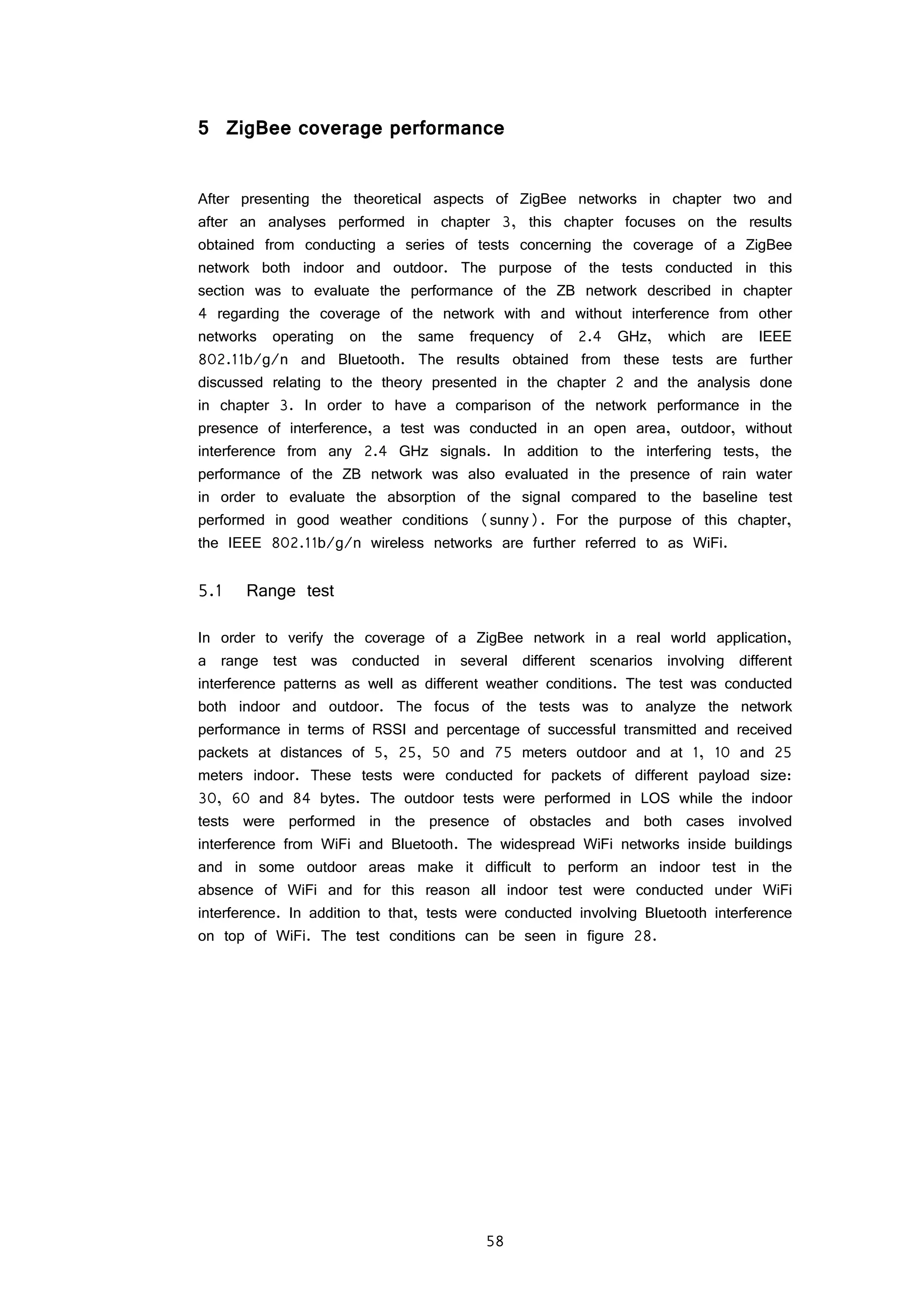
67. 59
Figure 30 ZigBee test conditions
The goal of the indoor tests was to measure the impact of obstacles on the RSSI
in both end device and coordinator as well as the PDR (Packet delivery ratio)
in the presence of WiFi and in some cases also Bluetooth. Obstacles in this
scenario were concrete walls and ceilings, but tests in LOS were also conducted
to measure the impact from interference only. The outdoor tests involved only LOS
and in some cases interference from WiFi as well as Bluetooth. Most of the
outdoor tests were performed in normal weather conditions of 15 degrees Celsius
with low humidity and one test was conducted in light rain conditions (drizzle) in
order to measure the RSSI and PDR in the presence of water for the 2.4 GHz
signal. Outdoor tests were conducted at several distances between the coordinator
and end device of 5, 25, 50 and 70 meters. Although the ZB specifications
enable devices to communicate up to 100 meters, the ZB capable devices (XBee)
from Digi International only allowed up to 75 meters and in some cases even
less. Tests performed outside this range did not return any result because the
devices could not detect each other. The indoor range specifications allow up to
40 m range [30]. One of the reasons for the lower coverage with this equipment
was the low transmission power of maximum 3 dBm (2 mW) as specified in the
XBee manual [30] which was the default highest power option. Security,
acknowledgements and encryption were not enabled for the purpose of this test.
Range test tool
The XBee modules that implement the ZigBee protocol stack used for coverage
evaluation in this project can be tested using the proprietary software from Digi
International called X-CTU. The software embeds a range test utility that measures
the real RF range and link quality between two radio modules within the same
network. The requirements for this test are a local device connected to a PC and
a remote device in the same network. Device selection is manual for the local
device, while the remote device can be discovered, an option that is available in

68. 60
ZigBee networks. The remote device can also be added to the network by manually
specifying the 16-bit or the 64-bit address. Figure 32 below shows the device
selection process as well as the MAC addresses of both devices. For the local
device, the protocol and the operating mode are also specified: in this case ZigBee
and API.
Figure 31 X-CTU device selection
The configuration options for the test are shown in figure 33. There are two types
of range tests:
 Cluster ID 0x12 – Any data sent to this cluster ID on the data
endpoint will be transmitted back to the sender, a more detailed view
can be seen in figure 33;
 Loopback – this test uses the serial port/USB hardware loopback
capabilities; this test requires AT mode of operation;
Figure 32 Cluster ID 0x12 mode of operation
After choosing the range test type, the packet payload can be configured, which
can be between 0 and 84 bytes out of the maximum 133 for a ZigBee packet.
The transmission interval (ms) and the reception timeout (ms) can be configured
as well. The minimum in both cases is 1000 ms with the available XBee modules.
The study performed in [53] shows that 1 packet/second is the optimal transmission
speed for >90% PDR.

69. 61
Figure 33 X-CTU session configuration
The test can be conducted for a limited number of packets as shown in figure
34 by setting the parameter with the same name or it can loop infinitely until
manually stopped. Finally the time window can be configured to show the desired
time intervals of the test which can be one minute, one hour or the whole time
period of the test.
After a test was conducted, data can be observed in the RSSI chart along with
the percentage of successful transmissions. An example of this chart is shown in
figure 35. Data in the chart can be disabled through the options on the bottom
of the chart as shown in the figure.
Figure 34 XCTU chart with RSSI and PDR
During a test the instant RSSI values in dBm of the last sent/received packet
can be seen as in figure 36.

70. 62
Figure 35 XCTU instant RSSI values
The packet summary after conducting a test can be seen in figure 37. It shows
the number of sent packets, received packets, transmission errors, lost packets
and returns the PDR.
Figure 36 XCTU PDR
The equipment needed for conducting this test is listed below:
 PC running X-CTU software
 USB cable
 XBee ZB Sensor
 XBee ZB module
 XBee adapter
5.2 Outdoor tests
The tests performed in this section were conducted in a park with no interference
from WiFi in order to evaluate the ZB network with only BL interference. The first
test in this section is the baseline test (no interference), followed by a test with
BL interference and a test in light rain so as to obtain results regarding the
attenuation of the signal in the presence of rain water.
Baseline test
As discussed in the previous chapters, the receiver sensitivity of the XBee ZB
modules used for this test are at -96 dBm with a transmit power of 2 mW (3
dBm). In order to obtain a baseline measurement for the ZigBee network coverage,

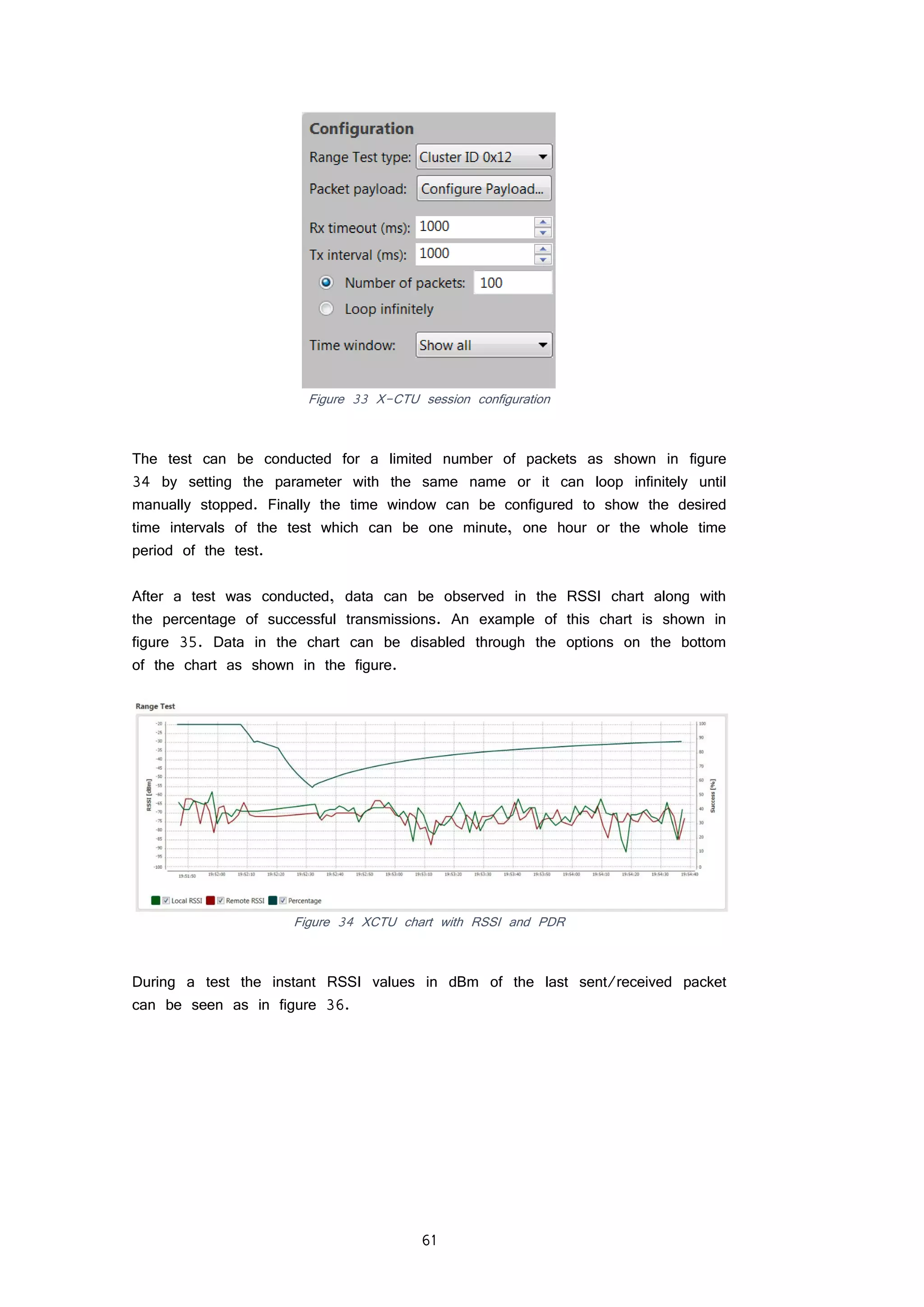
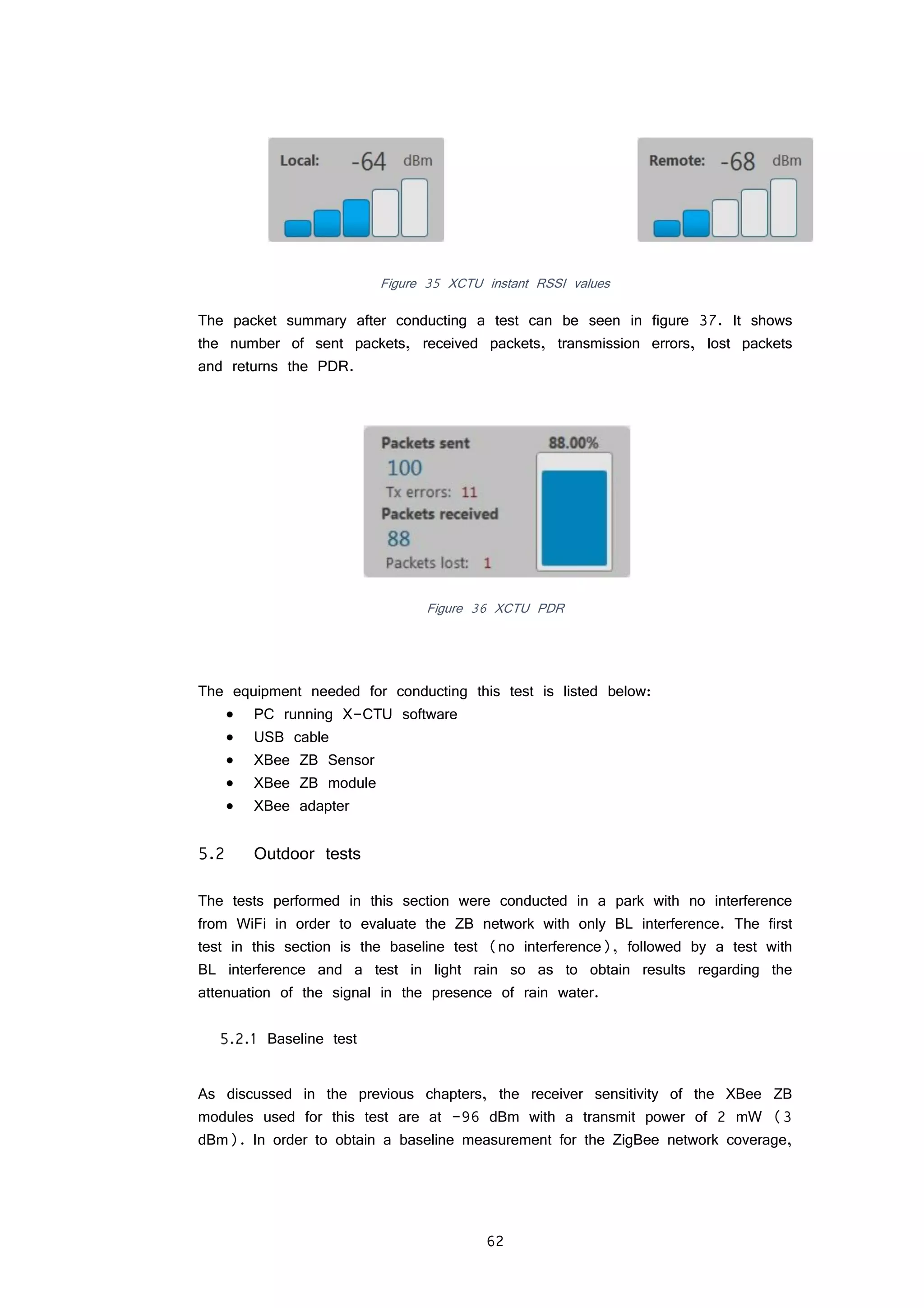
71. 63
an outdoor test in LOS without any interference was conducted. The weather
conditions were sunny with low humidity levels.
Test parameters:
 Test type: Cluster ID 0x12
 1 second transmit interval
 1 second receiver timeout
 100 packets
 Local/remote antenna height: 1 meter
Table 17 RSSI measurements and PDR for 30 bytes packet at several distances
Payload
size: 30
bytes
Distance [m] 5 25 50 75 85
PDR [%] 100 100 100 100 0
Average local RSSI
[dBm]
-52 -62 -69 -74 n/a
Average remote RSSI
[dBm]
-54 -64 -71 -76 n/a
Table 18 RSSI measurements and PDR for 60 bytes packet at several distances
Payload
size: 60
bytes
Distance [m] 5 25 50 75 85
PDR [%] 100 100 100 100 0
Average local RSSI
[dBm]
-53 -63 -72 -78 n/a
Average remote RSSI
[dBm]
-55 -65 -75 -80 n/a
Table 19 RSSI measurements and PDR for 84 bytes packet at several distances
Payload
size: 84
bytes
Distance [m] 5 25 50 75 85
PDR [%] 100 100 100 100 0
Average local RSSI
[dBm]
-54 -66 -75 -79 n/a
Average remote RSSI
[dBm]
-56 -69 -77 -80 n/a
The baseline test, as seen in the above tables, has resulted in 100% PDR on
all distances and for all payload sizes although the RSSI is decreasing according
the FSPL described in the link budget subsection in chapter three. Figure 38
below is showing the measured RSSI values at their corresponding distance between
the two ZB modules.

72. 64
Figure 37 Decreasing RSSI values in baseline ZB test for several distances
For a better understanding of the path loss model in this test, the FSPL was
calculated for the 2.4 GHz signal at the corresponding distances between the two
ZB modules and compared with the measured path loss. The comparison is shown
in figure 39, below.
Figure 38 Theoretical FSPL compared with measured average RSSI values for all packets
lengths
The path loss for the measured values was calculated using the following equation:

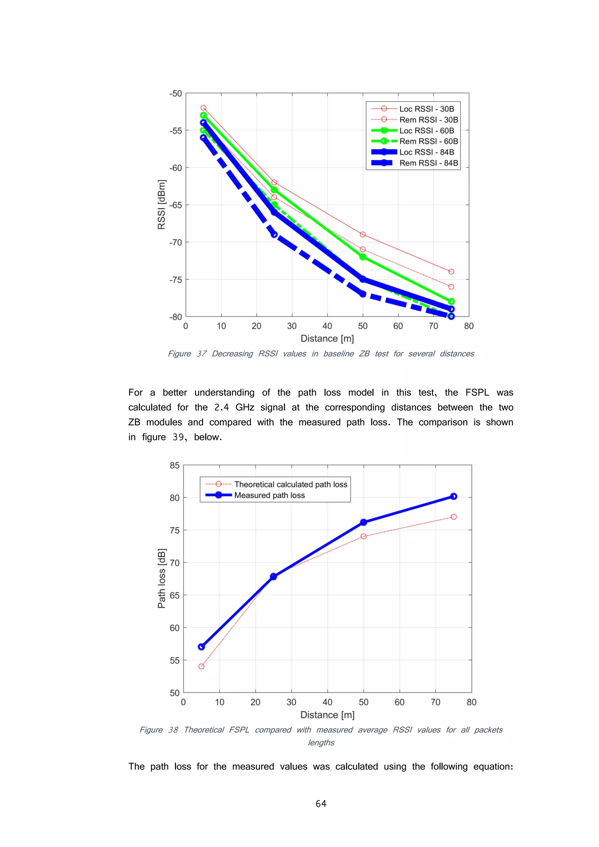
73. 65
𝑃𝑎𝑡ℎ 𝑙𝑜𝑠𝑠[𝑑𝐵] = 𝑂𝑢𝑡𝑝𝑢𝑡 𝑝𝑜𝑤𝑒𝑟[𝑑𝐵𝑚] − 𝐼𝑛𝑝𝑢𝑡 𝑝𝑜𝑤𝑒𝑟[𝑑𝐵𝑚]
Where the output power is the default transmission power of the XBee module
given in the XBee manual [30] which is 3 dBm (2mW) and the input power,
in this case, is the RSSI measured at the receiving XBee module. Using the
averaged RSSI measurements found in tables 17, 18 and 19 for the different
packet lengths, the path loss was calculated not taking into account other possible
losses with no power gain in the transmission. The minor error seen in the figure,
where the measured value is the same as the theoretical one for the 25 meters
distance, is probably given by a measurement error. Overall, the measured values
follow the FSPL described in chapter 3, although considering that the RF LOS
was not respected for the 50 and 75 meters distance, the path loss for the
measured values is slowly deviating from the reference theoretical path loss because
of the fading signals reaching the receiver.
Bluetooth interference
Following the baseline test conducted above, an interfering Bluetooth file transfer
was setup for the following test. The interfering BL connection was placed around
the ZB local device which, according to the BL specifications, only covers 10
meters around the transmitter. The weather conditions and parameters were the
same as the baseline test.
Test parameters:
 Test type: Cluster ID 0x12
 1 second transmit interval
 1 second receiver timeout
 100 packets
 Local/remote antenna height: 1 meter

Table 20 RSSI measurements and PDR for 30 bytes packet at several distances
Payload
size: 30
bytes
Distance [m] 5 25 50 75 85
PDR [%] 100 100 100 100 0
Average local RSSI
[dBm]
-53 -62 -70 -75 n/a
Average remote RSSI
[dBm]
-54 -63 -71 -76 n/a
Table 21 RSSI measurements and PDR for 60 bytes packet at several distances
Payload
size: 60
bytes
Distance [m] 5 25 50 75
PDR [%] 100 100 100 100 0
Average local RSSI
[dBm]
-55 -63 -72 -78 n/a
Average remote RSSI
[dBm]
-56 -65 -74 -79 n/a

74. 66
Table 22 RSSI measurements and PDR for 84 bytes packet at several distances
Payload
size: 84
bytes
Distance [m] 5 25 50 75 85
PDR [%] 100 100 100 99 0
Average local RSSI
[dBm]
-54 -64 -75 -80 n/a
Average remote RSSI
[dBm]
-55 -66 -76 -82 n/a
Figure 39 Decreasing RSSI values in BL interference test for several distances

75. 67
Figure 40 Average RSSI for baseline test compared with BL interference
In figure 41 above, the average RSSI for all packet lengths was calculated for
both baseline test and with BL interference to have a better comparison between
the two tests. The figure shows that there is not much difference in how the two
tests performed. One of the reasons for this is that there was not enough
interference from BL to cause a change in the results. BL uses FHSS to convey
information while ZB uses DSSS and the two techniques were both developed to
cope with heavy interference. The test involved only one BL transmission therefore
the interference could not be detected with only one transfer.
The results also show a link between packet size and RSSI and as the packet
length increases, the RSSI values for those packet lengths decreases. This
information is useful when deciding on a packet length in a ZB network. The
empirical study in [53] has shown that a 60 bytes packets length is optimal for
a PDR >90%, which corresponds to a payload size of 11 bytes, a sufficient
amount in 80% of IoT applications considering the Sigfox specifications of a
maximum payload size of 12 bytes [48, 69].
Regarding the BL interference test, the PDR was mostly not affected considering
that BL avoids the interfering channels using FHSS. The only difference in PDR
between the two tests was recorded for the 84 bytes packet at 75 m distance,
and the reason for this packet loss might not be related to the interference.
Although the tests were conducted in LOS, the RF LOS was not satisfied as the
antenna height was too low for the tests at 50 and 75 meters, which directly
affected the RSSI at those distances by introducing fading signals at the receivers,
as seen in figure 39.

76. 68
From the two tests conducted so far it can be concluded that in order to have
a significant impact from BL interference on the ZB network, more simultaneous
BL transmissions are required in order to obtain a comparable difference and a
definite result. The lack of testing equipment (BL transmissions) has been a
barrier to providing a more conclusive test result.
Effects of light rain and fading signals on the ZB network
There were two tests performed in this subsection with the first being conducted
during a light rain with fading signals and the other test was conducted in the
absence of rain also with fading signals. The same test parameters were considered
in order to observe the impact of rain in the overall signal power.
Test parameters of test during rain:
 Test type: Cluster ID 0x12
 1 second transmit interval
 1 second receiver timeout
 100 packets
 Local/remote antenna height: 0.5 meter
Table 23 RSSI measurements and PDR for 30 bytes packet at several distances
Payload
size: 30
bytes
Distance [m] 5 25 50 75
PDR [%] 100 99 8 0
Average local RSSI
[dBm]
-75 -84 -91 n/a
Average remote RSSI
[dBm]
-76 -86 -93 n/a
Table 24 RSSI measurements and PDR for 60 bytes packet at several distances
Payload
size: 60
bytes
Distance [m] 5 25 50 75
PDR [%] 100 97 1 0
Average local RSSI
[dBm]
-79 -85 -92 n/a
Average remote RSSI
[dBm]
-80 -87 -95 n/a
Table 25 RSSI measurements and PDR for 84 bytes packet at several distances
Payload
size: 84
bytes
Distance [m] 5 25 50 75
PDR [%] 98 95 0 0
Average local RSSI
[dBm]
-78 -80 n/a n/a
Average remote RSSI
[dBm]
-79 -81 n/a n/a

77. 69
From the results in the table above, it can be observed that for the 75 meters
test, the PDR is 0 for all packet lengths and the RSSI could not be measured.
The PDR drops significantly as the range increases and even small size payloads
of 30 bytes have only reached 8% at 50 meters, while for a payload size of 60
bytes at the same distance the PDR is 1% and 0% for 84 bytes. Taking into
account that the antenna height is rather small (0.5 meters) in this test, the
measurements shown in tables 23, 24 and 25 are considerably lower than the
ones from the baseline test in the previous subsection concerning RSSI. The low
antenna height resulted in enhanced fading signals in the ZB receivers which
directly affected the measured RSSI values. The other reason for this large
difference in RSSI is the rain itself which attenuated the signal strength and also
contributed to the inconsistent RSSI values at the same distance and different
packet lengths compared with the baseline test. The consequences of this low
RSSI values are also observed in the very low PDR for the 50 meter distance
in which case the values are very close to the receiver sensitivity of -96 dBm.
Comparing with the baseline test, the average RSSI is approximately 20 dBm
lower on all distances and for all packet lengths. This is shown below in figure
42, below.
Figure 41 Difference in average RSSI at 5, 25 and 50 m for baseline test and rain
As in the baseline test, the path loss in this scenario was calculated for the new
RSSI measurements affected by rain and fading. The comparison in dB between
the theoretical FSPL, the baseline scenario path loss and the rain scenario path
loss are shown in figure 43.

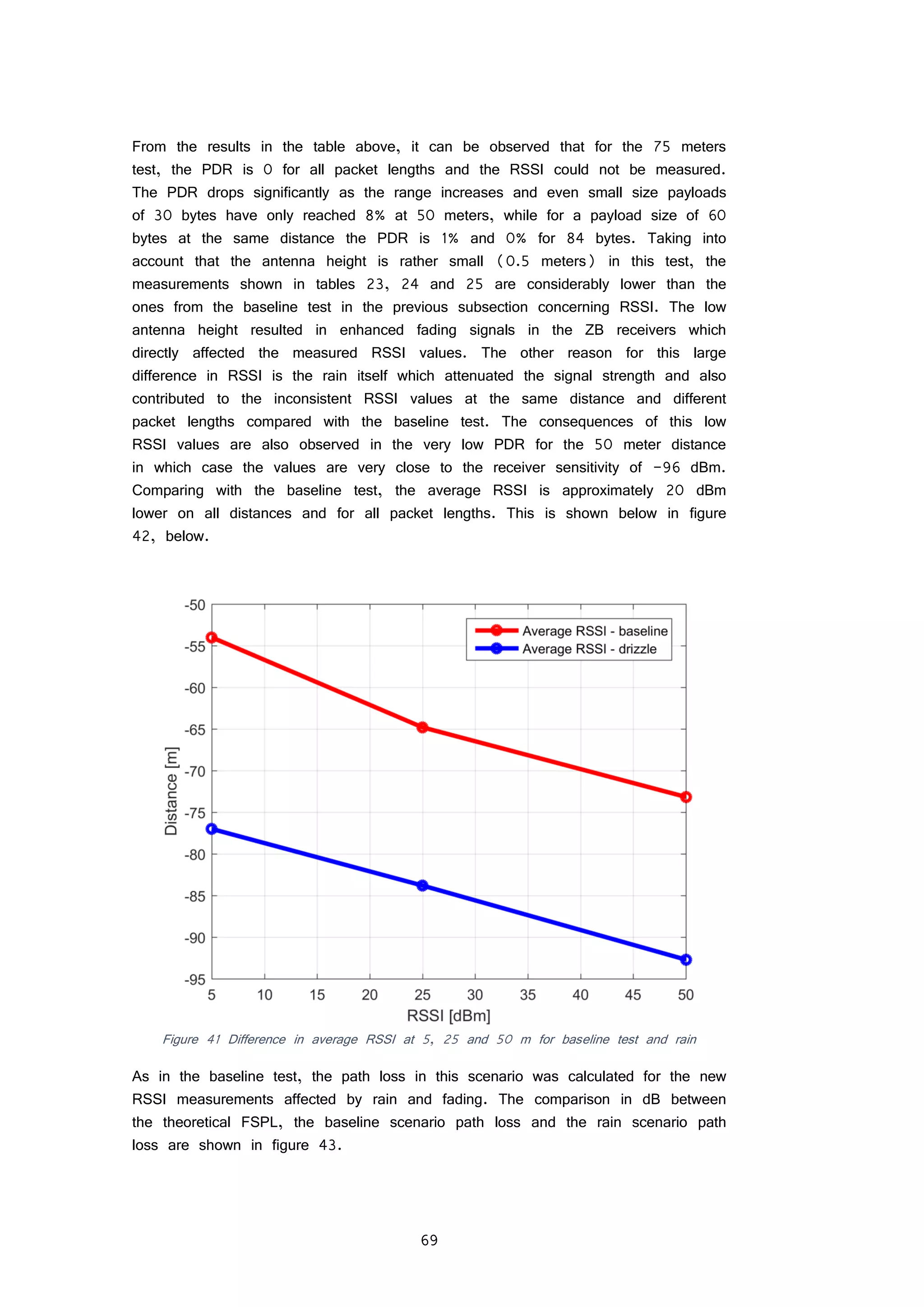
78. 70
Figure 42 Comparison between theoretical FSPL, baseline path loss and fading path loss
during rain
In order to have a better understanding between the differences in power absorption
of water compared with fading signals a second test was conducted in exactly the
same conditions as the test in this subsection but in the absence of rain. The
results are shown in the tables 26, 27 and 28.
Test parameters in the absence of rain:
 Test type: Cluster ID 0x12
 1 second transmit interval
 1 second receiver timeout
 100 packets
 Local/remote antenna height: 0.5 meter
Table 26 RSSI measurements and PDR for 30 bytes packet at several distances
Payload
size: 30
bytes
Distance [m] 5 25 50 75
PDR [%] 100 98 74 0
Average local RSSI
[dBm]
-67 -75 -85 n/a
Average remote RSSI
[dBm]
-65 -78 -86 n/a
Table 27 RSSI measurements and PDR for 60 bytes packet at several distances
Payload
size: 60
bytes
Distance [m] 5 25 50 75
PDR [%] 100 95 78 0
Average local RSSI
[dBm]
-68 -77 -87 n/a

79. 71
Average remote RSSI
[dBm]
-70 -79 -89 n/a
Table 28 RSSI measurements and PDR for 84 bytes packet at several distances
Payload
size: 84
bytes
Distance [m] 5 25 50 75
PDR [%] 100 98 24 0
Average local RSSI
[dBm]
-70 -80 -91 n/a
Average remote RSSI
[dBm]
-71 -81 -92 n/a
Comparing the two tests in this subsection in terms of PDR, the test in the
absence of rain resulted in an overall better PDR considering the 50 meters test
which is expected because of the overall higher RSSI values. The results from
these two tests were used to calculate the path loss and a comparison with path
losses from the baseline test as well as the theoretical FSPL are shown in figure
44. The results are conclusive to the fact that the largest impact on the RSSI
comes from fading signals rather than rain water. The fading signals accounted for
14.8 dB more in path loss on average compared with the baseline test while the
rain water accounts for only 6 dB more on average resulting in a total average
path loss of 20.8 dB more than the baseline test. This large path loss directly
affects the coverage of a network and efforts into choosing the right antenna height
should be emphasized for optimal results.
Figure 43 Comparison between theoretical FSPL, baseline path loss, fading path loss with and
without rain

80. 72
5.3 Indoor tests
The availability of WiFi mainly on the 2.4 GHz band on all channels and in most
of the buildings did not allow access to a test without this interference. This
section includes tests performed with interference from an idle WiFi network period
followed by a test with interference from a busy WiFi network and two more tests
from both WiFi and BL interference. Like in the outdoor test, the results presented
here are in the form of average RSSI of the local and remote devices as well
as the PDR on distances of 5, 10 and 20 meters. Considering that the test was
performed indoor, the different distances involved a different number of obstacles
in the form of concrete walls and kitchen cupboards (wooden walls and cupboard
contents). For the 5 meters test, the obstacle was in the form of a fire resistant
door, for the 10 meter test, there were 2 concrete walls and kitchen cupboards
and the test at 20 meters involved 5 walls and the kitchen cupboards.
Idle WiFi network interference
The operating channel for the ZB network is 17 which is interfering with WiFi
channel 6 (the most busy channel in the tested area) and the overlapping
channels around channel 6. The network channel availability for the WiFi network
was observed with a WiFi network analyzer that provided an overview of the
channels used in the test area. The test was conducted in an idle network period
in the early morning so as to benefit from as little interference as possible in
order to establish a baseline test. The results for this test are presented in tables
29, 30 and 31.
Test parameters:
 Test type: Cluster ID 0x12
 1 second transmit interval
 1 second receiver timeout
 100 packets
 Local antenna height: 1 meter
 Remote antenna height 1.5 meters
Table 29 RSSI measurements and PDR for 30 bytes packet at several distances
Payload
size: 30
bytes
Distance [m] 5 10 20 25
PDR [%] 100 100 98 0
Average local RSSI
[dBm]
-63 -75 -86 n/a
Average remote RSSI
[dBm]
-65 -76 -87 n/a

81. 73
Table 30 RSSI measurements and PDR for 60 bytes packet at several distances
Payload
size: 60
bytes
Distance [m] 5 10 20 25
PDR [%] 100 98 95 0
Average local RSSI
[dBm]
-66 -76 -88 n/a
Average remote RSSI
[dBm]
-68 -79 -89 n/a
Table 31 RSSI measurements and PDR for 84 bytes packet at several distances
Payload
size: 84
bytes
Distance [m] 5 10 20 25
PDR [%] 99 95 95 0
Average local RSSI
[dBm]
-67 -77 -87 n/a
Average remote RSSI
[dBm]
-69 -80 -89 n/a
Considering that the test was conducted in the early hours of the morning so as
to have as little WiFi interference as possible, the PDR rates do not drop below
95% in the worst case scenario of 20 meters distance with 84 bytes payload
size. The test at 25 meters and 6 concrete walls plus cupboards resulted in 0
PDR and the RSSI values could not be measured. The results are conclusive in
terms of maximum distance and number of obstacles in which packets could still
be recovered, that being 20 meters and 5 concrete walls for the ZB modules
used at the transmit power of 3 dBm. The decreasing RSSI values in this test
are shown in figure 45, below.

82. 74
Figure 44 RSSI measured values for indoor test with idle WiFi network interference
Busy WiFi network interference
The test conducted in this subsection has the objective of evaluating the performance
of the ZB network in the presence WiFi interference during heavy usage (evening).
Test parameters:
 Test type: Cluster ID 0x12
 1 second transmit interval
 1 second receiver timeout
 100 packets
 Local antenna height: 1 meter
 Remote antenna height 1.5 meters
Table 32 RSSI measurements and PDR for 30 bytes packet at several distances
Payload
size: 30
bytes
Distance [m] 5 10 20 25
PDR [%] 99 99 95 0
Average local RSSI
[dBm]
-67 -75 -86 n/a
Average remote RSSI
[dBm]
-68 -77 -88 n/a

83. 75
Table 33 RSSI measurements and PDR for 60 bytes packet at several distances
Payload
size: 60
bytes
Distance [m] 5 10 20 25
PDR [%] 97 92 89 0
Average local RSSI
[dBm]
-70 -77 -88
n/a
Average remote RSSI
[dBm]
-72 -79 -89
n/a
Table 34 RSSI measurements and PDR for 84 bytes packet at several distances
Payload
size: 84
bytes
Distance [m] 5 10 20 25
PDR [%] 98 93 85 0
Average local RSSI
[dBm]
-72 -80 -91
n/a
Average remote RSSI
[dBm]
-74 -82 -94
n/a
Figure 46 below shows the average RSSI values for the test conducted with
interference from a busy WiFi network.
Figure 45 RSSI values for indoor test with busy WiFi network interference
Looking at the two tests performed in this section, there are comparable differences
in both average RSSI values as well as PDR. In the idle WiFi interference test,
the lowest PDR was 95% while in the busy WiFi interference test the PDR
dropped as low as 85% for a maximum packet length and longest distance of 20
meters with most obstacles. One of the reasons behind these results is that the

84. 76
CSMA-CA mechanism used by the ZB network delayed the medium access times
for the ZB packets for more than 1 second, which is the maximum receiver timeout
set for this test, resulting in 10% less packets received in the worst case. Although
this mechanism works to avoid collisions, it is not perfect and packets may still
collide.
Previous work [78] in low power wireless networking has shown that interference
distorts the RSSI which is an important parameter in determining interference as a
cause of packet loss. At the same time, the lower received power (because of
listening and transmitting on the channel at the same time) directly influences the
coverage area for the network which is already quite limited in indoor environments.
The results also show that for shorter packets the impact of WiFi interference is
not as big in both PDR and RSSI given the shorter transmission time in which
case collisions are less likely to occur. The RSSI values gradually decrease as
the distance and number of obstacles increases and a comparison between the
averaged RSSI measurements from both tests are shown in figure 47.
Figure 46 Difference in RSSI for the idle and busy WiFi periods
Considering the path loss model for indoor environments described in chapter 3,
the path loss was calculated for the 2.4 GHz signal and compared with the
measured values for the two tests performed in this section. The results are
presented in figure 48 and the graph shows that the path loss model is respected
although the measured path loss for the two WiFi interference tests are, on
average for all distances, 6.9 dB and 9.8 dB more than the theoretical model.
As discussed in chapter 3, the path loss model for indoor environments may vary
due to different building materials and thickness of walls. Considering that the test
parameters and environment were the same in both WiFi tests, the difference in

85. 77
path loss between the idle and busy WiFi network of 2.9 dB can only be attributed
to the interference caused during the high usage of the WiFi network. The 2.9
dB difference is a direct cause of interference on the RSSI values, although it
does not represent a big influence and the consequences of this interference only
accounted for 10% less packets received compared to the idle WiFi network test.
As discussed before, the DSSS modulation technique used by ZB is efficient in
avoiding interference from other technologies using the 2.4 GHz band.
Figure 47 Comparison of path loss for the WiFi interference tests
Two more tests involving Bluetooth interference were conducted in this section on
top of the WiFi interference, but they resulted in very similar results making the
tests inconclusive in this case. In order to obtain a more significant impact of BL
for ZB networks, more transmissions are necessary to interfere with the ZB network.
5.4 Summary
This chapter was meant to show the reader a series of indoor and outdoor tests
that had the objective of analyzing the performance of the ZB network in different
indoor and outdoor scenarios including interference from WiFi and Bluetooth. The
performance was compared in terms of PDR and RSSI. The RSSI measured values
in all test were used to calculate the path loss in those scenarios and a comparison
was done with the theoretical path loss models described in chapter 3. In the
outdoor tests the conclusion is that fading has the most impact on signal strength
and efforts to avoid that should be emphasized. The signal strength is also affected
by rain, but to a smaller extent and the test was only run in a light rain, meaning
that further investigations must be done regarding heavy rain scenarios in order to

86. 78
have a definitive result. The impact of Bluetooth interference was inconclusive in
all tests because of the lack of testing equipment.
The indoor tests provided valuable data in evaluating the effects of interference on
signal strength and the overall conclusion is that WiFi does not present a major
interference problem. At the same time, out of the total 15% dropped packets in
the worst case test of maximum packet length, 20 meters and 5 concrete walls,
5% were attributed to losses due to indoor signal propagation and 10% to WiFi
interference. As mentioned before, the tests conducted here were done with no
retransmissions implemented in the ZB network and further research is required to
evaluate how the networks performs with this mechanism enabled as well as
security, encryption and a network with a larger number of nodes in order to have
a definite conclusion regarding actual throughput and the effects of WiFi and BL
interference with a larger network size. Coverage enhancements are also possible
with an increase in transmission power and a mesh topology. The XBee modules
used for these tests had a maximum transmit power of only 3 dBm (2 mW),
while other ZB capable devices can have up to 62 mW (18 dBm) which ca
effectively increase the maximum allowed path loss of the signal.
Although the tests are conclusive for a small network size involving two nodes, in
order to evaluate the coverage performance of the network in real world IoT
applications, more tests involving a larger number of nodes must be conducted.

87. 79
6 Conclusions
The goal of the report, as specified in the first chapter, was achieved through a
series of results that were meant to test the coverage performance of a ZigBee
network in indoor and outdoor environments and in the presence of interference
from WiFi and BL. Preceding these results, an analysis was conducted on coverage
and capacity regarding Sigfox, LTE-M and ZigBee in order to evaluate the impact
of those technologies in a IoT scenario.
The conclusion drawn from this report are meant to help the reader understand
the differences between current cellular networks like 2G, 3G and 4G/LTE which
are meant to facilitate voice communication and high data rates and the developing
LPWANs which are designed to support low data rates and M2M communication
with enhanced coverage. The different architectural designs were first highlighted in
chapter two and an initial conclusion was that mobile networks were not designed
to handle billions of M2M devices that are meant to sleep 99% of the time in
order to preserve battery life. Sigfox and Weightless have proven to be highly
competitive technologies that will accommodate most of the M2M devices that will
flood the network in the near future given their low cost solutions and fast
deployment. Most of the M2M devices that are currently deployed are supported
by 2G and 3G networks. The migration towards LTE-M is expected in the near
future, but at the same time the deployment of LTE networks and the high cost
of compatible LTE M2M devices are contributing to the slow migration towards this
network. LPWANs will play an important role in the first part of IoT deployments.
The biggest challenge in an IoT scenario will be in developing a new service
model because the current client-server model will become the bottleneck.
In the analysis performed in chapter three it was observed that the choice of
protocols plays a critical role in providing the required level of reliability and
functionality to IoT networks. Ultimately, the type of application will decide the use
of a specific technology in an optimal scenario when there is a choice. Data rates
as specified by the current long range technologies range from 100 bps for Sigfox
and up to 10 Mbps for Weightless, with LTE-M having up to 1 Mbps. The short
range technologies like ZigBee and Bluetooth will be more suitable for small to
medium sized IoT scenarios and are more comfortable and cheap to manage
because they are not bound to a network operator and monthly subscriptions. The
biggest challenges that will arise from using unlicensed spectrum in technologies
like Sigfox, Weightless, ZigBee and Bluetooth will be interference mitigation
techniques.
In chapter five the tests performed on a ZigBee network regarding coverage have
provided valuable information regarding the effect of fading signals and rain water
on signal strength and PDR. The results have shown that the biggest challenge
in providing a good coverage and PDR is in avoiding fading signals which is
something that can be accomplished relatively easy in a LOS environment while
rain water cannot be avoided in an outdoor scenario. The effects of WiFi interference

88. 80
in an indoor environment were not so severe, resulting in only 10% lost packets
as a consequence of interference only and 5% as a consequence of indoor signal
propagation in the worst case scenario of 20 meters distance and 5 concrete
walls with maximum packet length. For shorter packets, the consequences were
even less severe and only 3% of packets were lost due to WiFi interference and
2% due to indoor signal propagation. From these results the conclusions are that
shorter packet lengths present a higher reliability in the presence of interference
and fading signals, although further research is required to evaluate ZB networks
with security, encryption and acknowledgements enabled.
6.1 Future work
The ZigBee Alliance will soon release the ZigBee 3 protocol which has standardized
functionality on all layers and this will be a big advantage in providing a solution
with complete interoperability. The new protocol will enable the seamless interaction
between devices from different vendors. It is also worth evaluating the protocol for
the 868 MHz band in order to have a comparison in terms of coverage and data
rates.

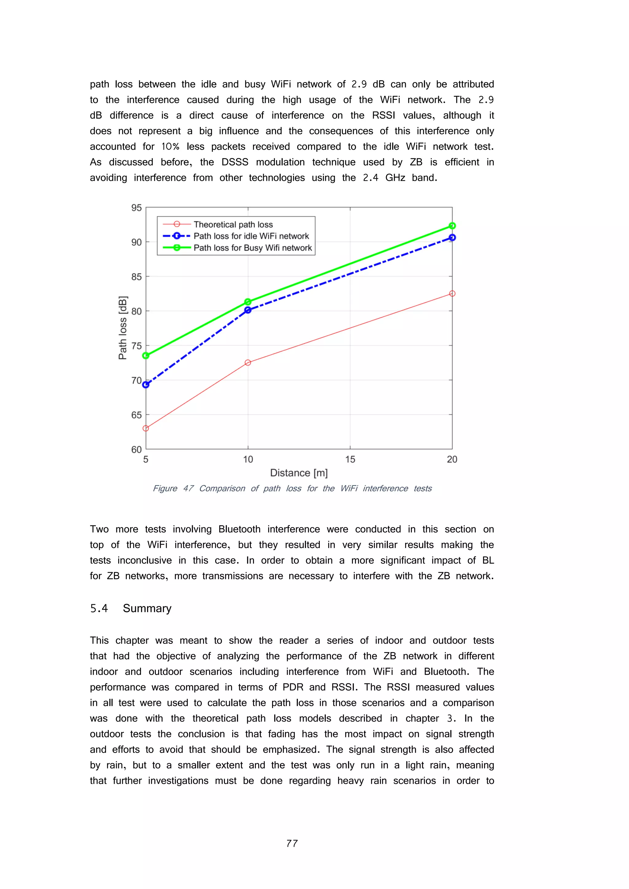
89. 81
7 Bibliography
[1] Wood, A. “The internet of things is revolutionising our lives, but standards
are a must” 2015 [Online] Available at:
http://www.theguardian.com/media-network/2015/mar/31/the-internet-of-things-
is-revolutionising-our-lives-but-standards-are-a-must (Accessed: 15 May 2015)
[2] Accessed: 25 March 2015 [Online] Available at:
https://www.raspberrypi.org/products/raspberry-pi-2-model-b/
[3] Accessed: 20 March 2015 [Online] Available at:
http://www.arm.com/products/processors/cortex-a/cortex-a7.php
[4] Accessed: 21 March 2015 [Online] Available at:
https://www.cooking-hacks.com/blog/learning-wireless-communication-zigbee
[5] C. Borean, “ZigBee Wireless Sensor Networks”, ETSI, December 15th
, Telecom
Italia, 2008 [Online] Available at:
https://docbox.etsi.org/Workshop/2008/200812_WIRELESSFACTORY/TELECOMIT
ALIA_Borean_ZIGBEE.pdf
[6] W. Kao, “Sensor Devices and Sensor Network Applications for the Smart
Grid/Smart Cities”, SensorsCon 2012, Santa Clara, CA, USA Available at:
http://www.iot-
summit.org/English/Archives/201203/Presentations/Bill_Kao_SensorsCon2012.pdf
[7] L. Doherty, J. Simon, T Watteyne, “Wireless Sensor Network Challenges and
Solutions”, Microwave Journal, August 2012 White paper
[8] Accessed: 12 April 2015 [Online] Available at:
http://www.sparqee.com/portfolio/sparqee-cell/
[9] Bonganay, A. C. D. et al, “Automated electric meter reading and monitoring
system using ZigBee-integrated raspberry Pi single board computer via Modbus”,
IEEE Students’ Conference on Electrical, Electronics and Computer Science, 2014
[12] Vujovic, V. and Maksimovic, M. (2014) “Raspberry Pi as a Wireless Sensor
node: Performances and constraints”, 37th International Convention on Information
and Communication Technology, Electronics and Microelectronics (MIPRO) 2014
[13] Ferdoush, S. and Li, X. “Wireless Sensor Network System Design Using
Raspberry Pi and Arduino for Environmental Monitoring Applications”, Procedia
Computer Science, 34, pp. 103–110. 2014
[14] Faludi, R. “Building Wireless Sensor Networks: With ZigBee, XBee, Arduino”
1st edn. United States: O’Reilly Media, Inc, USA. 2011
[15] Bell, C. “Beginning Sensor Networks with Arduino and Raspberry Pi” United
States: APress. 2014
[18] Sauter, M. “From GSM to LTE: An Introduction to Mobile Networks and
Mobile Broadband” 1st edn. United Kingdom: Wiley-Blackwell (an imprint of John
Wiley & Sons Ltd) 2011
[22] Accessed: 25 May 2015 [Online] “GPRS & EDGE” Available at:
http://www.3gpp.org/technologies/keywords-acronyms/102-gprs-edge
[25] Reid, T. “Essays on the intellectual powers of man” Edited by A D Woozley.
United States: Lincoln-Rembrandt Pub. 1986
[30] Digi International Inc., “XBee®/XBee-PRO® ZB RF Modules”, March 2012

90. 82
[32] Seo D., “The 1G (First Generation) Mobile Communication Technology
Standards”, 2013 Available at: http://www.igi-global.com/chapter/first-
generation-mobile-communications-technology/76774#chapter-preview
[33] Leon-Garcia, A. and Widjaja, I. “Communication networks: fundamental
concepts and key architectures”. United Kingdom: McGraw-Hill Education (ISE
Editions) 2002
[34] Accessed: 11 October 2015 [Online] “Dispelling LTE Myths” Available at:
http://www.3gpp.org/news-events/3gpp-news/1268-Dispelling-LTE-Myths
[36] Cisco “Cisco Visual Networking Index: Global Mobile Data Traffic Forecast
Update, 2014–2019”, February 3, 2015
[37] Accessed: 26 May 2015 [Online] Available at:
http://www.m2m-summit.com/files/jo_dressler_sierra_wireless_lte-changing_m2m-
world_2014.pdf 2014
[38] Nokia“LTE-M – Optimizing LTE for the Internet of Things”, White paper
2015
[39] Accessed: 28 May [Online] Available at:
http://www.3gpp.org/specifications/releases/68-release-12
[41] Accessed: 30 May 2015 [Online] “Bluetooth Low Energy” Available at:
https://developer.bluetooth.org/TechnologyOverview/Pages/BLE.aspx
[42] Atmel, “The Bluetooth Wireless Technology”, White paper, 2000
[43] Gomez, C., Oller, J. and Paradells, J. “Overview and Evaluation of Bluetooth
Low Energy: An Emerging Low-Power Wireless Technology”, Sensors, 12(12),
pp. 11734–11753, 2012
[44] Accessed: 17 September 2015 “Weightless-N” (2015) [Online] Available
at:
http://www.weightless.org/about/weightlessn
[45] Accessed: 25 September 2015 “Nwave Network” [Online] Available at:
http://www.nwave.io/nwave-network/
[46] Accessed: 25 September 2015 “Weightless-W” [Online] Available at:
http://www.weightless.org/about/weightlessw
[47] A. Woolhouse, “The Weightless Standard”, United Kingdom 2015
[48] SIGFOX, “Sigfox – One network A Billion Dreams”, White paper 2014
[49] Accessed: 29 September 2015 [Online] Available at:
http://www.sigfox.com/en/#!/technology
[50] R.S Hvindgelby, “Evaluating Protocols for the Internet of Things”, Bachelor
project 2015
[52] Tranzeo Wireless Technologies, “Wireless Link Budget Analysis”, White paper
2010
[53] N. Wisitpongphan, “Wireless Sensor Network Planning for Fingerprint based
Indoor Localization using ZigBee: Empirical Study”, Article 2005
[55] Accessed 23 September 2015 [Online] H. Im et al, “Multimedia Traffic Load
Distribution in Massively Multiplayer Online Games” Available at:
http://link.springer.com/chapter/10.1007%2F11919568_87#page-2
[56] H. Christiansen, “Mobile Network Planning”, 2014
[57] John C. Bicket, “Bit-rate Selection in Wireless Networks” 23-09-2015
[58] Accessed: 26 September 2015 “One day at SigFox” [Online] Available at:
http://www.disk91.com/2015/news/technologies/one-day-at-sigfox/

91. 83
[59] Accessed: 27 September 2015 [Online] Available at:
http://www.axsem.com/www/sigfox
[60] Accessed: 27 September 2015 [Online] Available at:
http://www.sigfox.com/en/#!/connected-world/sigfox-network-operator
[61] Link Labs, “A Comprehensive Look at Low Power, Wide Area Networks”,
White paper, 2015
[62], R. Ratasuk et al., “Recent Advancements in M2M Communications in 4G
Networks and Evolution Towards 5G”, Article 2015
[63] 3GPP TR 36.888, “Study on provision of low-cost Machine-Type
Communications (MTC) User Equipments (UEs) based on LTE”, v.12.0.0, June
2013
[64] Accessed: 29 September 2015 [Online] Available at:
http://www.etsi.org/deliver/etsi_en/300200_300299/30022001/02.04.01_40/en_
30022001v020401o.pdf
[65] Accessed: 11 October 2015 [Online] “The ZigBee Alliance | Control your
World” Available at: http://www.zigbee.org/
[66] Shin, S., Park, H., Choi, S. and Kwon, W. “Packet Error Rate Analysis
of ZigBee Under WLAN and Bluetooth Interferences”, IEEE Transactions on Wireless
Communications, 6(8), pp. 2825–2830. 2007
[67] Accessed: 30 September 2015 [Online] “Short Range Device” in Wikipedia.
Available at: https://en.wikipedia.org/wiki/Short_Range_Devices
[68] Accessed: 29 September 2015 [Online] “XBee-PRO 868 - Digi International”
Available at: http://www.digi.com/products/xbee-rf-solutions/modules/xbee-pro-
868#specifications
[69] C. Fourtet, “Keys for scalable M2M/IoT Networks”, 2014
[70] Accessed: 29 September 2015 [Online] Available at:
http://m2mworldnews.com/2012/06/25/31497-interview-with-sigfox-a-new-
operator-dedicated-to-m2m-and-iot-communications-2/
[71] Accessed: 29 September 2015 [Online] Available at:
http://www.gaussianwaves.com/2011/05/ebn0-vs-ber-for-bpsk-over-rayleigh-
channel-and-awgn-channel-2/
[72] A. Sudhir Babu and K.V. Sambasiva Rao, “Evaluation of BER for AWGN,
Rayleigh and Rician Fading Channels under Various Modulation Schemes”, Journal,
2011
[73] IEEE 802.16p-11/0014, “IEEE 802.16p Machine to Machine (M2M)
Evaluation Methodology Document (EMD)”, 2011
[74] Goldsmith, A. “Wireless communications”. Cambridge: Cambridge University
Press (Virtual Publishing). 2006
[75] Ratasuk, R., Tan, J. and Ghosh, A. “Coverage and Capacity Analysis for
Machine Type Communications in LTE”, 2012 IEEE 75th Vehicular Technology
Conference (VTC Spring), 2012
[76] ITU-R, “Propagation data and prediction methods for the planning of indoor
radio communication systems and the radio local area networks in the frequency
range 300 MHz to 100 GHz, ITU-R Recommendations”, Geneva, 2015. Available
at:
https://www.itu.int/dms_pubrec/itu-r/rec/p/R-REC-P.1238-8-201507-I!!PDF-
E.pdf

92. 84
[77] B. R. Jadhavar, T. R. Sontakke, “2.4 GHz Propagation Prediction Models
for Indoor Wireless Communications Within Building”, Article 2012
[78] R. Maheshwari, S. Jain, and S. R. Das, “Proceedings of the third ACM
international workshop on Wireless network testbeds, experimental evaluation and
characterization” New York, NY, USA, 2008

93. 85
Annex A
#include "arduPi.h"
#include "iostream"
#include "fstream"
#include "iomanip"
#include "bitset"
using namespace std;
int incomingByte = 0;
SerialPi sb;
char myChar = '/';
char buffer[128];
char light[2];
char hum[2];
char temp[2];
void setup()
{
memset(buffer, '0', sizeof(buffer));
sb.begin(9600);
}
void loop()
{
ofstream myfile;
ofstream myfile2;
ofstream myfile3;
delay(20);
incomingByte = sb.readBytesUntil(myChar, buffer,
sizeof(buffer));
myfile.open("SizeofBuffer.txt");
myfile << incomingByte;
delay(100);
myfile.close();
myfile2.open("BinaryBuffer.txt", ios::out |
ios::binary);
for (int i = 0; i < 28; i++)
{
myfile2 << bitset<8>(buffer[i]);
delay(100);
}
myfile2.close();
delay(20);
delay(100);
myfile3.open("LHT.txt", ios::out | ios::binary);
for (int j = 21; j < 27; j++)
{
myfile3 << bitset<8>(buffer[j]);
}
myfile3.close();
delay(20);
}
int main ()
{
setup();
while(1)

94. 86
{
while(sb.available() > 0)
{
loop();
}
}
return (0);
}