Descriptive Statistics

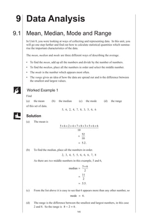
1. 145
MEP Pupil Text 9
9 Data Analysis
9.1 Mean, Median, Mode and Range
In Unit 8, you were looking at ways of collecting and representing data. In this unit, you
will go one step further and find out how to calculate statistical quantities which summa-
rise the important characteristics of the data.
The mean, median and mode are three different ways of describing the average.
• To find the mean, add up all the numbers and divide by the number of numbers.
• To find the median, place all the numbers in order and select the middle number.
• The mode is the number which appears most often.
• The range gives an idea of how the data are spread out and is the difference between
the smallest and largest values.
Worked Example 1
Find
(a) the mean (b) the median (c) the mode (d) the range
of this set of data.
5, 6, 2, 4, 7, 8, 3, 5, 6, 6
Solution
(a) The mean is
5 6 2 4 7 8 3 5 6 6
10
+ + + + + + + + +
=
52
10
= 5 2
. .
(b) To find the median, place all the numbers in order.
2, 3, 4, 5, 5, 6, 6, 6, 7, 8
As there are two middle numbers in this example, 5 and 6,
median =
+
5 6
2
=
11
2
= 5 5
. .
(c) From the list above it is easy to see that 6 appears more than any other number, so
mode = 6.
(d) The range is the difference between the smallest and largest numbers, in this case
2 and 8. So the range is 8 2 6
− = .

2. 146
MEP Pupil Text 9
Worked Example 2
Five people play golf and at one hole their scores are
3, 4, 4, 5, 7.
For these scores, find
(a) the mean (b) the median (c) the mode (d) the range .
Solution
(a) The mean is
3 4 4 5 7
5
+ + + +
=
23
5
= 4 6
. .
(b) The numbers are already in order and the middle number is 4. So
median = 4.
(c) The score 4 occurs most often, so,
mode = 4.
(d) The range is the difference between the smallest and largest numbers, in this case
3 and 7, so
range = −
7 3
= 4.
Exercises
1. Find the mean median, mode and range of each set of numbers below.
(a) 3, 4, 7, 3, 5, 2, 6, 10
(b) 8, 10, 12, 14, 7, 16, 5, 7, 9, 11
(c) 17, 18, 16, 17, 17, 14, 22, 15, 16, 17, 14, 12
(d) 108, 99, 112, 111, 108
(e) 64, 66, 65, 61, 67, 61, 57
(f) 21, 30, 22, 16, 24, 28, 16, 17
2. Twenty children were asked their shoe sizes. The results are given below.
8, 6, 7, 6, 5, 4 1
2
, 7 1
2
, 6 1
2
, 8 1
2
, 10
7, 5, 5 1
2
8, 9, 7, 5, 6, 8 1
2
6
For this data, find
(a) the mean (b) the median (c) the mode (d) the range.
9.1

3. 147
MEP Pupil Text 9
3. Eight people work in a shop. They are paid hourly rates of
£2, £15, £5, £4, £3, £4, £3, £3.
(a) Find
(i) the mean (ii) the median (iii) the mode.
(b) Which average would you use if you wanted to claim that the staff were:
(i) well paid (ii) badly paid?
(c) What is the range?
4. Two people work in a factory making parts for cars. The table shows how many
complete parts they make in one week.
Worker Mon Tue Wed Thu Fri
Fred 20 21 22 20 21
Harry 30 15 12 36 28
(a) Find the mean and range for Fred and Harry.
(b) Who is most consistent?
(c) Who makes the most parts in a week?
5. A gardener buys 10 packets of seeds from two different companies. Each pack
contains 20 seeds and he records the number of plants which grow from each pack.
Company A 20 5 20 20 20 6 20 20 20 8
Company B 17 18 15 16 18 18 17 15 17 18
(a) Find the mean, median and mode for each company's seeds.
(b) Which company does the mode suggest is best?
(c) Which company does the mean suggest is best?
(d) Find the range for each company's seeds.
6. Adrian takes four tests and scores the following marks.
65, 72, 58, 77
(a) What are his median and mean scores?
(b) If he scores 70 in his next test, does his mean score increase or decrease?
Find his new mean score.
(c) Which has increased most, his mean score or his median score?
7. Richard keeps a record of the number of fish he catches over a number of fishing
trips. His records are:
1, 0, 2, 0, 0, 0, 12, 0, 2, 0, 0, 1, 18, 0, 2, 0, 1.
(a) Why does he object to talking about the mode and median of the number of
fish caught?

4. 148
MEP Pupil Text 9
(b) What are the mean and range of the data?
(c) Richard's friend, Najir, also goes fishing. The mode of the number of fish
he has caught is also 0 and his range is 15.
What is the largest number of fish that Najir has caught?
8. A garage owner records the number of cars which visit his garage on 10 days.
The numbers are:
204, 310, 279, 314, 257, 302, 232, 261, 308, 217.
(a) Find the mean number of cars per day.
(b) The owner hopes that the mean will increase if he includes the number of
cars on the next day. If 252 cars use the garage on the next day, will the
mean increase or decrease?
9. The children in a class state how many children there are in their family.
The numbers they state are given below.
1, 2, 1, 3, 2, 1, 2, 4, 2, 2, 1, 3, 1, 2,
2, 2, 1, 1, 7, 3, 1, 2, 1, 2, 2, 1, 2, 3
(a) Find the mean, median and mode for this data.
(b) Which is the most sensible average to use in this case?
10. The mean number of people visiting Jane each day over a five-day period is 8.
If 10 people visit Jane the next day, what happens to the mean?
11. The table shows the maximum and minimum temperatures recorded in six cities
one day last year.
City Maximum Minimum
Los Angeles 22°C 12°C
Boston 22°C − °
3 C
Moscow 18°C − °
9 C
Atlanta 27°C 8°C
Archangel 13°C − °
15 C
Cairo 28°C 13°C
(a) Work out the range of temperature for Atlanta.
(b) Which city in the table had the lowest temperature?
(c) Work out the difference between the maximum temperature and the
minimum temperature for Moscow.
(LON)
12. The weights, in grams, of seven potatoes are
260, 225, 205, 240, 232, 205, 214.
What is the median weight?
(SEG)
9.1

5. 149
MEP Pupil Text 9
13. Here are the number of goals scored by a school football team in their matches this
term.
3, 2, 0, 1, 2, 0, 3, 4, 3, 2
(a) Work out the mean number of goals.
(b) Work out the range of the number of goals scored.
(LON)
14.
(a) The weights, in kilograms, of the 8 members of Hereward House tug of war
team at a school sports are:
75, 73, 77, 76, 84, 76, 77, 78.
Calculate the mean weight of the team.
(b) The 8 members of Nelson House tug of war team have a mean weight of
64 kilograms.
Which team do you think will win a tug of war between Hereward House
and Nelson House? Give a reason for your answer.
(MEG)
15. Pupils in Year 8 are arranged in eleven classes. The class sizes are
23, 24, 24, 26, 27, 28, 30, 24, 29, 24, 27.
(a) What is the modal class size?
(b) Calculate the mean class size.
The range of the class sizes for Year 9 is 3.
(c) What does this tell you about the class sizes in Year 9 compared with those
in Year 8?
(SEG)
16. A school has to select one pupil to take part in a General Knowledge Quiz.
Kim and Pat took part in six trial quizzes. The following lists show their scores.
Kim 28 24 21 27 24 26
Pat 33 19 16 32 34 18
Kim had a mean score of 25 with a range of 7.
(a) Calculate Pat's mean score and range.
(b) Which pupil would you choose to represent the school? Explain the reason
for your choice, referring to the mean scores and ranges.
(MEG)
Information
The study of statistics was begun by an English mathematician, John Graunt (1620–1674).
He collected and studied the death records in various cities in Britain and, despite the fact
that people die randomly, he was fascinated by the patterns he found.

6. 150
MEP Pupil Text 9
17. Eight judges each give a mark out of 6 in an ice-skating competition.
Oksana is given the following marks.
5.3, 5.7, 5.9, 5.4, 4.5, 5.7, 5.8, 5.7
The mean of these marks is 5.5, and the range is 1.4.
The rules say that the highest mark and the lowest mark are to be deleted.
5.3, 5.7, 5.9, 5.4, 4.5, 5.7, 5.8, 5.7
(a) (i) Find the mean of the six remaining marks.
(ii) Find the range of the six remaining marks.
(b) Do you think it is better to count all eight marks, or to count only the six
remaining marks? Use the means and the ranges to explain your answer.
(c) The eight marks obtained by Tonya in the same competition have a mean
of 5.2 and a range of 0.6. Explain why none of her marks could be as high
as 5.9.
9.2 Finding the Mean from Tables and
Tally Charts
Often data are collected into tables or tally charts. This section considers how to find the
mean in such cases.
Worked Example 1
A football team keep records of the number of goals it scores per match during a season.
No. of Goals Frequency
0 8
1 10
2 12
3 3
4 5
5 2
Find the mean number of goals per match.
Solution
The table above can
be used, with a third
column added.
The mean can now
be calculated.
Mean =
73
40
= 1 825
. .
No. of Goals Frequency No. of Goals × Frequency
0 8 0 8 0
× =
1 10 1 10 10
× =
2 12 2 12 24
× =
3 3 3 3 9
× =
4 5 4 5 20
× =
5 2 5 2 10
× =
TOTALS 40 73
(Total matches) (Total goals)
9.1
(MEG)

7. 151
MEP Pupil Text 9
Worked Example 2
The bar chart shows how many cars were sold by a salesman over a period of time.
Find the mean number of cars sold per day.
Solution
The data can be transferred to a table and a third column included as shown.
Mean =
50
20
= 2 5
.
Worked Example 3
A police station kept records of the number of road traffic accidents in their area each day
for 100 days. The figures below give the number of accidents per day.
1 4 3 5 5 2 5 4 3 2 0 3 1 2 2 3 0 5 2 1
3 3 2 6 2 1 6 1 2 2 3 2 2 2 2 5 4 4 2 3
3 1 4 1 7 3 3 0 2 5 4 3 3 4 3 4 5 3 5 2
4 4 6 5 2 4 5 5 3 2 0 3 3 4 5 2 3 3 4 4
1 3 5 1 1 2 2 5 6 6 4 6 5 8 2 5 3 3 5 4
Find the mean number of accidents per day.
0 1 2 3 4 5
1
2
3
4
5
6
Frequency
Cars sold per day
Cars sold daily Frequency Cars sold × Frequency
0 2 0 2 0
× =
1 4 1 4 4
× =
2 3 2 3 6
× =
3 6 3 6 18
× =
4 3 4 3 12
× =
5 2 5 2 10
× =
TOTALS 20 50
(Total days) (Total number of cars sold)

8. 152
MEP Pupil Text 9
Solution
The first step is to draw out and complete a tally chart. The final column shown below
can then be added and completed.
Number of Accidents Tally Frequency No. of Accidents × Frequency
0 |||| 4 0 4 0
× =
1 |||| |||| 10 1 10 10
× =
2 |||| |||| |||| |||| || 22 2 22 44
× =
3 |||| |||| |||| |||| ||| 23 3 23 69
× =
4 |||| |||| |||| | 16 4 16 64
× =
5 |||| |||| |||| || 17 5 17 85
× =
6 |||| | 6 6 6 36
× =
7 | 1 7 1 7
× =
8 | 1 8 1 8
× =
TOTALS 100 323
Mean number of accidents per day =
323
100
= 3 23
. .
Exercises
1. A survey of 100 households asked how many cars there were in each household
The results are given below.
No. of Cars Frequency
0 5
1 70
2 21
3 3
4 1
Calculate the mean number of cars per household.
2. The survey of question 1 also asked how many TV sets there were in each house-
hold. The results are given below.
No. of TV Sets Frequency
0 2
1 30
2 52
3 8
4 5
5 3
Calculate the mean number of TV sets per household.
9.2

9. 153
MEP Pupil Text 9
3. A manager keeps a record of the number of calls she makes each day on her mobile
phone.
Number of calls
per day 0 1 2 3 4 5 6 7 8
Frequency 3 4 7 8 12 10 14 3 1
Calculate the mean number of calls per day.
4. A cricket team keeps a record of the number of runs scored in each over.
No. of Runs Frequency
0 3
1 2
2 1
3 6
4 5
5 4
6 2
7 1
8 1
Calculate the mean number of runs per over.
5. A class conduct an experiment in biology. They place a number of 1m by 1m
square grids on the playing field and count the number of worms which appear
when they pour water on the ground. The results obtained are given below.
6 3 2 1 3 2 1 3 0 1
0 3 2 1 1 4 0 1 2 0
1 1 2 2 2 4 3 1 1 1
2 3 3 1 2 2 2 1 7 1
(a) Calculate the mean number of worms.
(b) How many times was the number of worms seen greater than the mean?
6. As part of a survey, a station recorded the number of trains which were late each
day. The results are listed below.
0 1 2 4 1 0 2 1 1 0
1 2 1 3 1 0 0 0 0 5
2 1 3 2 0 1 0 1 2 1
1 0 0 3 0 1 2 1 0 0
Construct a table and calculate the mean number of trains which were late each
day.

10. 154
MEP Pupil Text 9
7. Hannah drew this bar chart to show the number of repeated cards she got when she
opened packets of football stickers.
Calculate the mean number of repeats per packet.
8. In a season a football team scored a total of 55 goals. The table below gives a
summary of the number of goals per match.
Goals per Match Frequency
0 4
1 6
2
3 8
4 2
5 1
(a) In how many matches did they score 2 goals?
(b) Calculate the mean number of goals per match.
9. A traffic warden is trying to work out the mean number of parking tickets he has
issued per day. He produced the table below, but has accidentally rubbed out some
of the numbers.
Fill in the missing numbers and calculate the mean.
Number of repeats
2
4
6
8
10
12
0 1 2 3 4 5 6
q
y
Frequency
Tickets per day Frequency No. of Tickets × Frequency
0 1
1 1
2 10
3 7
4 20
5 2
6
TOTALS 26 72
9.2

11. 155
MEP Pupil Text 9
10. Here are the weights, in kg, of 30 students.
45, 52, 56, 65, 34, 45, 67, 65, 34, 45, 65, 87, 45, 34, 56,
54, 45, 67, 84, 45, 67, 45, 56, 76, 57, 84, 35, 64, 58, 60
(a) Copy and complete the frequency table below using a class interval of 10
and starting at 30.
Weight Range (w) Tally Frequency
30 40
≤ <
w
(b) Which class interval has the highest frequency?
(LON)
11. The number of children per family in a recent survey of 21 families is shown.
1 2 3 2 2 4 2 2
3 2 2 2 3 2 2 2
4 1 2 3 2
(a) What is the range in the number of children per family?
(b) Calculate the mean number of children per family. Show your working.
A similar survey was taken in 1960.
In 1960 the range in the number of children per family was 7 and the mean was 2.7.
(c) Describe two changes that have occurred in the number of children per
family since 1960.
(SEG)
9.3 Calculations with the Mean
This section considers calculations concerned with the mean, which is usually taken to
be the most important measure of the average of a set of data.
Worked Example 1
The mean of a sample of 6 numbers is 3.2. An extra value of 3.9 is included in the
sample. What is the new mean?

12. 156
MEP Pupil Text 9
Solution
Total of original numbers = ×
6 3 2
.
= 19 2
.
New total = +
19 2 3 9
. .
= 23 1
.
New mean =
23 1
7
.
= 3 3
.
Worked Example 2
The mean number of a set of 5 numbers is 12.7. What extra number must be added to
bring the mean up to 13.1?
Solution
Total of the original numbers = ×
5 12 7
.
= 63 5
.
Total of the new numbers = ×
6 13 1
.
= 78 6
.
Difference = −
78 6 63 5
. .
= 15 1
.
So the extra number is 15.1.
Exercises
1. The mean height of a class of 28 students is 162 cm. A new girl of height 149 cm
joins the class. What is the mean height of the class now?
2. After 5 matches the mean number of goals scored by a football team per match is
1.8. If they score 3 goals in their 6th match, what is the mean after the 6th match?
3. The mean number of children ill at a school is 3.8 per day, for the first 20 school
days of a term. On the 21st day 8 children are ill. What is the mean after 21 days?
4. The mean weight of 25 children in a class is 58 kg. The mean weight of a second
class of 29 children is 62 kg. Find the mean weight of all the children.
5. A salesman sells a mean of 4.6 conservatories per day for 5 days. How many must
he sell on the sixth day to increase his mean to 5 sales per day?
6. Adrian's mean score for four tests is 64%. He wants to increase his mean to 68%
after the fifth test. What does he need to score in the fifth test?
7. The mean salary of the 8 people who work for a small company is £15 000. When
an extra worker is taken on this mean drops to £14 000. How much does the new
worker earn?
9.3

13. 157
MEP Pupil Text 9
8. The mean of 6 numbers is 12.3. When an extra number is added, the mean changes
to 11.9. What is the extra number?
9. When 5 is added to a set of 3 numbers the mean increases to 4.6. What was the
mean of the original 3 numbers?
10. Three numbers have a mean of 64. When a fourth number is included the mean is
doubled. What is the fourth number?
9.4 Mean, Median and Mode for Grouped Data
The mean and median can be estimated from tables of grouped data.
The class interval which contains the most values is known as the modal class.
Worked Example 1
The table below gives data on the heights, in cm, of 51 children.
Class Interval 140 150
≤ <
h 150 160
≤ <
h 160 170
≤ <
h 170 180
≤ <
h
Frequency 6 16 21 8
(a) Estimate the mean height. (b) Estimate the median height.
(c) Find the modal class.
Solution
(a) To estimate the mean, the mid-point of each interval should be used.
Class Interval Mid-point Frequency Mid-point × Frequency
140 150
≤ <
h 145 6 145 6 870
× =
150 160
≤ <
h 155 16 155 16 2480
× =
160 170
≤ <
h 165 21 165 21 3465
× =
170 180
≤ <
h 175 8 175 8 1400
× =
Totals 51 8215
Mean =
8215
51
= 161 (to the nearest cm)
(b) The median is the 26th value. In this case it lies in the 160 170
≤ <
h class interval.
The 4th value in the interval is needed. It is estimated as
160
4
21
10 162
+ × = (to the nearest cm)
(c) The modal class is 160 170
≤ <
h as it contains the most values.

14. 158
MEP Pupil Text 9
Also note that when we speak of someone by age, say 8, then the person could be any age
from 8 years 0 days up to 8 years 364 days (365 in a leap year!). You will see how this is
tackled in the following example.
Worked Example 2
The age of children in a primary school were recorded in the table below.
Age 5 – 6 7 – 8 9 – 10
Frequency 29 40 38
(a) Estimate the mean. (b) Estimate the median. (c) Find the modal age.
Solution
(a) To estimate the mean, we must use the mid-point of each interval; so, for example
for '5 – 6', which really means
5 7
≤ <
age ,
the mid-point is taken as 6.
Class Interval Mid-point Frequency Mid-point × Frequency
5 – 6 6 29 6 29 174
× =
7 – 8 8 40 8 40 320
× =
9 – 10 10 38 10 38 380
× =
Totals 107 874
Mean =
874
107
= 8 2
. (to 1 decimal place)
(b) The median is given by the 54th value, which we have to estimate. There are 29
values in the first interval, so we need to estimate the 25th value in the second
interval. As there are 40 values in the second interval, the median is estimated as
being
25
40
of the way along the second interval. This has width 9 7 2
− = years, so the
median is estimated by
25
40
2 1 25
× = .
from the start of the interval. Therefore the median is estimated as
7 1 25 8 25
+ =
. . years.
(c) The modal age is the 7 – 8 age group.
9.4

15. 159
MEP Pupil Text 9
Worked Example 1 uses what are called continuous data, since height can be of any value.
(Other examples of continuous data are weight, temperature, area, volume and time.)
The next example uses discrete data, that is, data which can take only a particular value,
such as the integers 1, 2, 3, 4, . . . in this case.
The calculations for mean and mode are not affected but estimation of the median
requires replacing the discrete grouped data with an approximate continuous interval.
Worked Example 3
The number of days that children were missing from school due to sickness in one year
was recorded.
Number of days off sick 1 – 5 6 – 10 11 – 15 16 – 20 21 – 25
Frequency 12 11 10 4 3
(a) Estimate the mean (b) Estimate the median. (c) Find the modal class.
Solution
(a) The estimate is made by assuming that all the values in a class interval are equal to
the midpoint of the class interval.
Class Interval Mid-point Frequency Mid-point × Frequency
1–5 3 12 3 12 36
× =
6–10 8 11 8 11 88
× =
11–15 13 10 13 10 130
× =
16–20 18 4 18 4 72
× =
21–25 23 3 23 3 69
× =
Totals 40 395
Mean =
395
40
= 9 925
. days.
(b) As there are 40 pupils, we need to consider the mean of the 20th and 21st values.
These both lie in the 6–10 class interval, which is really the 5.5–10.5 class interval,
so this interval contains the median.
As there are 12 values in the first class interval, the median is found by considering
the 8th and 9th values of the second interval.
As there are 11 values in the second interval, the median is estimated as being
8 5
11
.
of the way along the second interval.

16. 160
MEP Pupil Text 9
But the length of the second interval is 10 5 5 5 5
. .
− = , so the median is estimated by
8 5
11
5 3 86
.
.
× =
from the start of this interval. Therefore the median is estimated as
5 5 3 86 9 36
. . .
+ = .
(c) The modal class is 1–5, as this class contains the most entries.
Exercises
1. A door to door salesman keeps a record of the number of homes he visits each day.
Homes visited 0 – 9 10 – 19 20 – 29 30 – 39 40 – 49
Frequency 3 8 24 60 21
(a) Estimate the mean number of homes visited.
(b) Estimate the median.
(c) What is the modal class?
2. The weights of a number of students were recorded in kg.
Mean (kg) 30 35
≤ <
w 35 40
≤ <
w 40 45
≤ <
w 45 50
≤ <
w 50 55
≤ <
w
Frequency 10 11 15 7 4
(a) Estimate the mean weight. (b) Estimate the median.
(c) What is the modal class?
3. A stopwatch was used to find the time that it took a group of children to run 100 m.
Time (seconds) 10 15
≤ <
t 15 20
≤ <
t 20 25
≤ <
t 25 30
≤ <
t
Frequency 6 16 21 8
(a) Is the median in the modal class? (b) Estimate the mean.
(c) Estimate the median.
(d) Is the median greater or less than the mean?
4. The distances that children in a year group travelled to school is recorded.
Distance (km) 0 0 5
≤ <
d . 0 5 1 0
. .
≤ <
d 1 0 1 5
. .
≤ <
d 1 5 2 0
. .
≤ <
d
Frequency 30 22 19 8
(a) Does the modal class contain the median?
(b) Estimate the median and the mean.
(c) Which is the largest, the median or the mean?
9.4

17. 161
MEP Pupil Text 9
5. The ages of the children at a youth camp are summarised in the table below.
Age (years) 6 – 8 9 – 11 12 – 14 15 – 17
Frequency 8 22 29 5
Estimate the mean age of the children.
6. The lengths of a number of leaves collected for a project are recorded.
Length (cm) 2 – 5 6 – 10 11 – 15 16 – 25
Frequency 8 20 42 12
Estimate (a) the mean (b) the median length of a leaf.
7. The table shows how many nights people spend at a campsite.
Number of nights 1 – 5 6 – 10 11 – 15 16 – 20 21 – 25
Frequency 20 26 32 5 2
(a) Estimate the mean. (b) Estimate the median.
(c) What is the modal class?
8. (a) A teacher notes the number of correct answers given by a class on
a multiple-choice test.
Correct answers 1 – 10 11 – 20 21 – 30 31 – 40 41 – 50
Frequency 2 8 15 11 3
(i) Estimate the mean. (ii) Estimate the median.
(iii) What is the modal class?
(b) Another class took the same test. Their results are given below.
Correct answers 1 – 10 11 – 20 21 – 30 31 – 40 41 – 50
Frequency 3 14 20 2 1
(i) Estimate the mean. (ii) Estimate the median.
(iii) What is the modal class?
(c) How do the results for the two classes compare?
Information
A quartile is one of 3 values (lower quartile, median and upper quartile) which divides
data into 4 equal groups.
A percentile is one of 99 values which divides data into 100 equal groups.
The lower quartile corresponds to the 25th percentile. The median corresponds to the
50th percentile. The upper quartile corresponds to the 75th percentile.

18. 162
MEP Pupil Text 9
9. 29 children are asked how much pocket money they were given last week.
Their replies are shown in this frequency table.
Pocket money Frequency
£ f
0 1 00
– £ . 12
£ . – £ .
1 01 2 00 9
£ . – £ .
2 01 3 00 6
£ . – £ .
3 01 4 00 2
(a) Which is the modal class?
(b) Calculate an estimate of the mean amount of pocket money received per child.
(NEAB)
10. The graph shows the number of hours a sample of people spent viewing television
one week during the summer.
(a) Copy and complete the frequency table for this sample.
Viewing time Number of
(h hours) people
0 10
≤ <
h 13
10 20
≤ <
h 27
20 30
≤ <
h 33
30 40
≤ <
h
40 50
≤ <
h
50 60
≤ <
h
(b) Another survey is carried out during the winter. State one difference you
would expect to see in the data.
(c) Use the mid-points of the class intervals to calculate the mean viewing time
for these people. You may find it helpful to use the table below.
10
20
30
40
0 10 20 30 40 50 60 70
Number of
people
Viewing time (hours)
9.4

19. 163
MEP Pupil Text 9
Viewing time Mid-point ×
(h hours) Mid-point Frequency Frequency
0 10
≤ <
h 5 13 65
10 20
≤ <
h 15 27 405
20 30
≤ <
h 25 33 825
30 40
≤ <
h 35
40 50
≤ <
h 45
50 60
≤ <
h 55
(SEG)
11. In an experiment, 50 people were asked to estimate the length of a rod to the
nearest centimetre. The results were recorded.
Length (cm) 20 21 22 23 24 25 26 27 28 29
Frequency 0 4 6 7 9 10 7 5 2 0
(a) Find the value of the median. (b) Calculate the mean length.
(c) In a second experiment another 50 people were asked to estimate the length
of the same rod. The most common estimate was 23 cm. The range of the
estimates was 13 cm.
Make two comparisons between the results of the two experiments.
(SEG)
12. The following list shows the maximum daily temperature, in °F , throughout the
month of April.
56.1 49.4 63.7 56.7 55.3 53.5 52.4 57.6 59.8 52.1
45.8 55.1 42.6 61.0 61.9 60.2 57.1 48.9 63.2 68.4
55.5 65.2 47.3 59.1 53.6 52.3 46.9 51.3 56.7 64.3
(a) Copy and complete the grouped frequency table below.
Temperature, T Frequency
40 50
< ≤
T
50 54
< ≤
T
54 58
< ≤
T
58 62
< ≤
T
62 70
< ≤
T
(b) Use the table of values in part (a) to calculate an estimate of the mean of this
distribution. You must show your working clearly.
(c) Draw a histogram to represent your distribution in part (a).
(MEG)

20. 164
MEP Pupil Text 9
9.5 Cumulative Frequency
Cumulative frequencies are useful if more detailed information is required about a set of
data. In particular, they can be used to find the median and inter-quartile range.
The inter-quartile range contains the middle 50% of the sample and describes how
spread out the data are. This is illustrated in Example 2.
Worked Example 1
For the data given in the table, draw up a
cumulative frequency table and then draw
a cumulative frequency graph.
Solution
The table below shows how to calculate
the cumulative frequencies.
Height (cm) Frequency Cumulative Frequency
90 100
< ≤
h 5 5
100 110
< ≤
h 22 5 22 27
+ =
110 120
< ≤
h 30 27 30 57
+ =
120 130
< ≤
h 31 57 31 88
+ =
130 140
< ≤
h 18 88 18 106
+ =
140 150
< ≤
h 6 106 6 112
+ =
A graph can then be plotted using points as shown below.
0
20
40
60
80
100
120
90 100 110 120 130 140 150
q
y
(90,0) (100,5)
(110,27)
(120,57)
(130,88)
(140,106)
(150,112)
Height (cm)
Cumulative
Frequency
Height (cm) Frequency
90 100
< ≤
h 5
100 110
< ≤
h 22
110 120
< ≤
h 30
120 130
< ≤
h 31
130 140
< ≤
h 18
140 150
< ≤
h 6

21. 165
MEP Pupil Text 9
Note
A more accurate graph is found by drawing a smooth curve through the points, rather
than using straight line segments.
Worked Example 2
The cumulative frequency graph below gives the results of 120 students on a test.
Cumulative
Frequency
0
20
40
60
80
100
120
90 100 110 120 130 140 150
(90,0) (100,5)
(110,27)
(120,57)
(130,88)
(140,106)
(150,112)
Height (cm)
0
20
40
60
80
100
120
20 40 60 80 100
0
Test Score
Cumulative
Frequency

22. 166
MEP Pupil Text 9
Use the graph to find:
(a) the median score, (b) the inter-quartile range,
(c) the mark which was attained by only 10% of the students,
(d) the number of students who scored more than 75 on the test.
Solution
(a) Since 1
2
of 120 is 60, the median
can be found by starting at 60
on the vertical scale, moving
horizontally to the graph line
and then moving vertically
down to meet the horizontal scale.
In this case the median is 53.
(b) To find out the inter-quartile range, we must consider the middle 50% of the
students.
To find the lower quartile,
start at 1
4
of 120, which is 30.
This gives
Lower Quartile = 43.
To find the upper quartile,
start at 3
4
of 120, which is 90.
This gives
Upper Quartile = 67.
The inter-quartile range is then
Inter - quartile Range Upper Quartile Lower Quartile
= −
= −
67 43
= 24.
Cumulative
Frequency
Score
0
20
40
60
80
100
120
20 40 60 80 100
0
Start at 60
Median = 53
Cumulative
Frequency
0
20
40
60
80
100
120
20 40 60 80 100
0
30
90
Lower quartile = 43
Upper quartile = 67
Test Score
9.5

23. 167
MEP Pupil Text 9
(c)
Here the mark which was attained
by the top 10% is required.
10 120 12
% of =
so start at 108 on the cumulative
frequency scale.
This gives a mark of 79.
(d) To find the number of students who
scored more than 75, start at 75 on
the horizontal axis.
This gives a cumulative frequency
of 103.
So the number of students with a
score greater than 75 is
120 103 17
− = .
As in Worked Example 1, a more accurate estimate for the median and inter-quartile
range is obtained if you draw a smooth curve through the data points.
Exercises
1. Make a cumulative frequency table for each set of data given below. Then draw a
cumulative frequency graph and use it to find the median and inter-quartile range.
(a) John weighed each apple in a large box. His results are given in this table.
Weight of
apple (g) 60 80
< ≤
w 80 100
< ≤
w 100 120
< ≤
w 120 140
< ≤
w 140 160
< ≤
w
Frequency 4 28 33 27 8
(b) Pasi asked the students in his class how far they travelled to school each day.
His results are given below.
Distance (km) 0 1
< ≤
d 1 2
< ≤
d 2 3
< ≤
d 3 4
< ≤
d 4 5
< ≤
d 5 6
< ≤
d
Frequency 5 12 5 6 5 3
0
20
40
60
80
100
120
20 40 60 80 100
0
79
108
Test Score
Cumulative
Frequency
Cumulative
Frequency
0
20
40
60
80
100
120
20 40 60 80 100
0
75
103
Test Score

24. 168
MEP Pupil Text 9
(c) A P.E. teacher recorded the distances children could reach in the long jump
event. His records are summarised in the table below.
Length of jump (m) 1 2
< ≤
d 2 3
< ≤
d 3 4
< ≤
d 4 5
< ≤
d 5 6
< ≤
d
Frequency 5 12 5 6 5
2. A farmer grows a type of wheat in two different fields. He takes a sample of
50 heads of corn from each field at random and weighs the grains he obtains.
Mass of grain (g) 0 5
< ≤
m 5 10
< ≤
m 10 15
< ≤
m 15 20
< ≤
m 20 25
< ≤
m 25 30
< ≤
m
Frequency Field A 3 8 22 10 4 3
Frequency Field B 0 11 34 4 1 0
(a) Draw cumulative frequency graphs for each field.
(b) Find the median and inter-quartile range for each field.
(c) Comment on your results.
3. A consumer group tests two types of batteries using a personal stereo.
Lifetime (hours) 2 3
< ≤
l 3 4
< ≤
l 4 5
< ≤
l 5 6
< ≤
l 6 7
< ≤
l 7 8
< ≤
l
Frequency Type A 1 3 10 22 8 4
Frequency Type B 0 2 2 38 6 0
(a) Use cumulative frequency graphs to find the median and inter-quartile range
for each type of battery.
(b) Which type of battery would you recommend and why?
4. The table below shows how the height of girls of a certain age vary. The data was
gathered using a large-scale survey.
Height (cm) 50 55
< ≤
h 55 60
< ≤
h 60 65
< ≤
h 65 70
< ≤
h 70 75
< ≤
h 75 80
< ≤
h 80 85
< ≤
h
Frequency 100 300 2400 1300 700 150 50
A doctor wishes to be able to classify children as:
Category Percentage of Population
Very Tall 5%
Tall 15%
Normal 60%
Short 15%
Very short 5%
Use a cumulative frequency graph to find the heights of children in each category.
9.5

25. 169
MEP Pupil Text 9
5. The manager of a double glazing company employs 30 salesmen. Each year he
awards bonuses to his salesmen.
Bonus Awarded to
£500 Best 10% of salesmen
£250 Middle 70% of salesmen
£ 50 Bottom 20% of salesmen
The sales made during 1995 and 1996 are shown in the table below.
Value of sales
(£1000) 0 100
< ≤
V 100 200
< ≤
V 200 300
< ≤
V 300 400
< ≤
V 400 500
< ≤
V
Frequency 1996 0 2 15 10 3
Frequency 1995 2 8 18 2 0
Use cumulative frequency graphs to find the values of sales needed to obtain each
bonus in the years 1995 and 1996.
6. The histogram shows the cost of buying a particular toy in a number of different
shops.
(a) Draw a cumulative frequency graph and use it to answer the following
questions.
(i) How many shops charged more than £2.65?
(ii) What is the median price?
(iii) How many shops charged less than £2.30?
(iv) How many shops charged between £2.20 and £2.60?
(v) How many shops charged between £2.00 and £2.50?
(b) Comment on which of your answers are exact and which are estimates.
2.00 2.20 2.40 2.60 2.80 3.00
0
1
2
3
4
5
6
7
Price (£)
Frequency

26. 170
MEP Pupil Text 9
7. Laura and Joy played 40 games of golf together. The table below shows Laura's
scores.
Scores (x) 70 80
< ≤
x 80 90
< ≤
x 90 100
< ≤
x 100 110
< ≤
x 110 120
< ≤
x
Frequency 1 4 15 17 3
(a) On a grid similar to the one below, draw a cumulative frequency diagram to
show Laura's scores.
(b) Making your method clear, use your graph to find
(i) Laura's median score,
(ii) the inter-quartile range of her scores.
(c) Joy's median score was 103. The inter-quartile range of her scores was 6.
(i) Who was the more consistent player?
Give a reason for your choice.
(ii) The winner of a game of golf is the one with the lowest score.
Who won most of these 40 games? Give a reason for your choice.
(NEAB)
8. A sample of 80 electric light bulbs was taken. The lifetime of each light bulb was
recorded. The results are shown below.
Lifetime (hours) 800– 900– 1000– 1100– 1200– 1300– 1400–
Frequency 4 13 17 22 20 4 0
Cumulative Frequency 4 17
(a) Copy and complete the table of values for the cumulative frequency.
(b) Draw the cumulative frequency curve, using a grid as shown below.
Cumulative
Frequency
60 70 80 90 100 110 120
10
20
30
40
q
y
Score
9.5

27. 171
MEP Pupil Text 9
(c) Use your graph to estimate the number of light bulbs which lasted more than
1030 hours.
(d) Use your graph to estimate the inter-quartile range of the lifetimes of the
light bulbs.
(e) A second sample of 80 light bulbs has the same median lifetime as the first
sample. Its inter-quartile range is 90 hours. What does this tell you about
the difference between the two samples?
(SEG)
9. The numbers of journeys made by a group of people using public transport in one
month are summarised in the table.
Number of journeys 0–10 11–20 21–30 31–40 41–50 51–60 61–70
Number of people 4 7 8 6 3 4 0
(a) Copy and complete the cumulative frequency table below.
Number of journeys ≤10 ≤20 ≤30 ≤ 40 ≤50 ≤60 ≤ 70
Cumulative frequency
(b) (i) Draw the cumulative frequency graph, using a grid as below.
10 20 30 40 50 60 70
10
0
20
30
40
q
y
Cumulative
Frequency
800 900 1000 1100 1200 1300 1400 1500
20
10
0
30
40
50
60
70
80
90
q
y
Lifetime (hours)
Cumulative
Frequency
Number of journeys

28. 172
MEP Pupil Text 9
(ii) Use your graph to estimate the median number of journeys.
(iii) Use your graph to estimate the number of people who made more than
44 journeys in the month.
(c) The numbers of journeys made using public transport in one month, by
another group of people, are shown in the graph.
Make one comparison between the numbers of journeys made by these
two groups.
(SEG)
10. The cumulative frequency graph below gives information on the house prices in
1992. The cumulative frequency is given as a percentage of all houses in England.
This grouped frequency table gives the percentage distribution of house prices (p)
in England in 1993.
10 20 30 40 50 60 70
10
0
20
30
40
Number of journeys
Cumulative
Frequency
0
20
40
60
80
100
240000
200000
100000
i
q
y
(
)
Cumulative
Frequency
House prices in 1992 (£)
9.5

29. 173
MEP Pupil Text 9
House prices (p) Percentage of houses
in pounds 1993 in this class interval
0 40 000
≤ <
p 26
40 000 52 000
≤ <
p 19
52 000 68000
≤ <
p 22
68000 88000
≤ <
p 15
88000 120 000
≤ <
p 9
120 000 160 000
≤ <
p 5
160 000 220 000
≤ <
p 4
(a) Use the data above to complete the cumulative frequency table below.
House prices (p) Cumulative
in pounds 1993 Frequency (%)
0 40 000
≤ <
p
0 52 000
≤ <
p
0 68000
≤ <
p
0 88000
≤ <
p
0 120 000
≤ <
p
0 160 000
≤ <
p
0 220 000
≤ <
p
(b) Trace or photocopy the grid for 1992, and on it construct a cumulative
frequency graph for your table for 1993.
(c) In 1992 the price of a house was £100 000. Use both cumulative frequency
graphs to estimate the price of this house in 1993. Make your method clear.
(LON)
11. The lengths of a number of nails were measured to the nearest 0.01 cm, and the
following frequency distribution was obtained.
Length of nail Number of nails Cumulative Frequency
(x cm)
0 98 1 00
. .
≤ <
x 2
1 00 1 02
. .
≤ <
x 4
1 02 1 04
. .
≤ <
x 10
1 04 1 06
. .
≤ <
x 24
1 06 1 08
. .
≤ <
x 32
1 08 1 10
. .
≤ <
x 17
1 10 1 12
. .
≤ <
x 7
1 12 1 14
. .
≤ <
x 4

30. 174
MEP Pupil Text 9
(a) Complete the cumulative frequency column.
(b) Draw a cumulative frequency diagram on a grid similar to the one below.
Use your graph to estimate
(i) the median length of the nails (ii) the inter-quartile range.
(NEAB)
12. A wedding was attended by 120 guests. The distance, d miles, that each guest
travelled was recorded in the frequency table below.
Distance
(d miles) 0 10
< ≤
d 10 20
< ≤
d 20 30
< ≤
d 30 50
< ≤
d 50 100
< ≤
d 100 140
< ≤
d
Number of
guests 26 38 20 20 12 4
(a) Using the mid-interval values, calculate an estimate of the mean distance
travelled.
(b) (i) Copy and complete the cumulative frequency table below.
Distance
(d miles) d ≤ 10 d ≤ 20 d ≤ 30 d ≤ 50 d ≤ 100 d ≤ 140
Number of
guests 120
(ii) On a grid similar to that shown below, draw a cumulative frequency
curve to represent the information in the table.
0 0.98 1.00 1.02 1.04 1.06 1.08 1.10 1.12 1.14
20
40
60
80
100
Cumulative
Frequency
Length of nail (cm)
9.5
Just for Fun
Comment on this statement. "Students who smoke perform worse academically than non-
smokers, so smoking will make you stupid."

31. 175
MEP Pupil Text 9
(c) (i) Use the cumulative frequency curve to estimate the median distance
travelled by the guests.
(ii) Give a reason for the large difference between the mean distance and
the median distance.
(MEG)
9.6 Standard Deviation
The two frequency polygons drawn on the graph below show samples which have the
same mean, but the data in one are much more spread out than in the other.
The range (highest value – lowest value) gives a simple measure of how much the data
are spread out.
Cumulative
Frequency
0 20 40 60 80 100 120 140
20
40
60
80
100
120
Distance travelled (miles)
Frequency
0 1 2 3 4 5 6 7 8 9 10 11 12
5
10
15
20
25
Length

32. 176
MEP Pupil Text 9
Standard deviation (s.d.) is a much more useful measure and is given by the formula:
s.d. =
−
=
∑ ( )
x x
n
i
i
n
2
1
where xi represents each datapoint x x xn
1 2
, , ...,
( )
x is the mean,
n is the number of values.
Then ( )
x x
i − 2
gives the square of the difference between each value and the mean
(squaring exaggerates the effect of data points far from the mean and gets rid of negative
values), and
( )
x x
i
i
n
−
=
∑ 2
1
sums up all these squared differences.
The expression
1 2
1
n
x x
i
i
n
−
( )
=
∑
gives an average value to these differences. If all the data were the same, then each xi
would equal x and the expression would be zero.
Finally we take the square root of the expression so that the dimensions of the standard
deviation are the same as those of the data.
So standard deviation is a measure of the spread of the data. The greater its value, the
more spread out the data are. This is illustrated by the two frequency polygons shown
above. Although both sets of data have the same mean, the data represented by the
'dotted' frequency polygon will have a greater standard deviation than the other.
Worked Example 1
Find the mean and standard deviation of the numbers,
6, 7, 8, 5, 9.
Solution
The mean, x , is given by,
x =
+ + + +
6 7 8 5 9
5
=
35
5
= 7.
9.6

33. 177
MEP Pupil Text 9
Now the standard deviation can be calculated.
s.d. =
− + − + − + − + −
( ) ( ) ( ) ( ) ( )
6 7 7 7 8 7 5 7 9 7
5
2 2 2 2 2
=
+ + + +
1 0 1 4 4
5
=
10
5
= 2
= 1 414
. (to 3 decimal places)
An alternative formula for standard deviation is
s.d. = −
=
∑x
n
x
i
i
n
2
1 2
This expression is much more convenient for calculations done without a calculator. The
proof of the equivalence of this formula is given below although it is beyond the scope of
the GCSE syllabus.
Proof
You can see the proof of the equivalence of the two formulae by noting that
x x x x x x
i
i
n
i i
i
n
−
( ) = − +
( )
= =
∑ ∑
2
1
2 2
1
2
= − ( ) +
= =
=
∑ ∑
∑
x x x x
i
i
n
i
i
n
i
n
2
1
2
1
1
2
= − +
= = =
∑ ∑ ∑
x x x x
i
i
n
i
i
n
i
n
2
1 1
2
1
2 1
(since the expressions 2x and x2
are common for each term in the summation).
But 1
1
i
n
n
=
∑ = , since you are summing 1 1 1
+ + + =
...
n
n
terms
1 2
4
4 3
44
, and x
n
x
i
n
=
=
∑
1
1
, by
definition, thus
1 1
2
2
1
2
1 1
2
n
x x
n
x x x x n
i
i
n
i
i
n
i
i
n
−
( ) = − +






= = =
∑ ∑ ∑ (substituting 1
1
=
=
∑ n
i
n
)

34. 178
MEP Pupil Text 9
= −












+
= =
∑ ∑
x
n
x
x
n
x
i
i
n
i
i
n
2
1 1 2
2 (dividing by n)
= − +
=
∑x
n
x x
i
i
n
2
1 2 2
2 (substituting x for
x
n
i
i
n
=
∑
1
)
= −
=
∑x
n
x
i
i
n
2
1 2
and the result follows.
Worked Example 2
Find the mean and standard deviation of each of the following sets of numbers.
(a) 10, 11, 12, 13, 14 (b) 5, 6, 12, 18, 19
Solution
(a) The mean, x , is given by
x =
+ + + +
10 11 12 13 14
5
=
60
5
= 12
The standard deviation can now be calculated using the alternative formula.
s.d. =
+ + + +





 −
10 11 12 13 14
5
12
2 2 2 2 2
2
= −
146 144
= 32
= 1 414
. (to 3 decimal places).
(b) The mean, x , is given by
x =
+ + + +
5 6 12 18 19
5
= 12 (as in part (a)).
9.6

35. 179
MEP Pupil Text 9
The standard deviation is given by
s.d. =
+ + + +





 −
5 6 12 18 19
5
12
2 2 2 2 2
2
= −
178 144
= 5 831
. (to 3 decimal places).
Note that both sets of numbers have the same mean value, but that set (b) has a much
larger standard deviation. This is expected, as the spread in set (b) is clearly far more
than in set (a).
Worked Example 3
The table below gives the number of road traffic accidents per day in a small town.
Accidents per day 0 1 2 3 4 5 6
Frequency 5 8 6 3 2 1 1
Find the mean and standard deviation of this data.
Solution
The necessary calculations for each datapoint, xi , are set out below.
Accidents per day Frequency
xi
( ) fi
( ) xi
2
x f
i i x f
i i
2
0 5 0 0 0
1 8 1 8 8
2 6 4 12 24
3 3 9 9 27
4 2 16 8 32
5 0 25 0 0
6 1 36 6 36
TOTALS 25 43 127
From the totals,
n = 25, x f
i i
i
n
=
∑ =
1
43, xi
i
n
2
1
127
=
∑ = .
The mean, x , is now given by
x
x f
n
i i
i
n
= =
∑
1
=
43
25
= 1 72
. .

36. 180
MEP Pupil Text 9
The standard deviation is now given by
s.d. = −
=
∑x f
n
x
i i
i
n
2
1 2
= −
127
25
1 722
.
= 1 457
. .
Most scientific calculators have statistical functions which will calculate the mean and
standard deviation of a set of data.
Exercises
1. (a) Find the mean and standard deviation of each set of data given below.
A 51 56 51 49 53 62
B 71 76 71 69 73 82
C 102 112 102 98 106 124
(b) Describe the relationship between each set of numbers and also the relation-
ship between their means and standard deviations.
2. Two machines, A and B, fill empty packets with soap powder. A sample of boxes
was taken from each machine and the weight of powder (in kg) was recorded.
A 2.27 2.31 2.18 2.2 2.26 2.24
B 2.78 2.62 2.61 2.51 2.59 2.67 2.62 2.68 2.70
(a) Find the mean and standard deviation for each machine.
(b) Which machine is most consistent?
3. Two groups of students were trying to find the acceleration due to gravity.
Each group conducted 5 experiments.
Group A 9.4 9.6 10.2 10.8 10.1
Group B 9.5 9.7 9.6 9.4 9.8
Find the mean and standard deviation for each group, and comment on their results.
4. The number of matches per box was counted for 100 boxes of matches.
The results are given in the table below.
9.6

37. 181
MEP Pupil Text 9
Number of Matches Frequency
44 28
45 31
46 14
47 15
48 8
49 2
50 2
Find the mean and standard deviation of this data.
5. When two dice were thrown 50 times the total scores shown below were obtained.
Score Frequency
2 1
3 0
4 4
5 8
6 12
7 9
8 7
9 5
10 3
11 1
12 0
Find the mean and standard deviation of these scores.
6. The length of telephone calls from an office was recorded. The results are given in
the table below.
Length of call (mins) 0 0 5
< ≤
t . 0 5 1 0
. .
< ≤
t 1 0 2 0
. .
< ≤
t 2 0 5 0
. .
< ≤
t
Frequency 8 10 12 4
Estimate the mean and standard deviation using this table.
7. The charges (to the nearest £) made by a garage for repair work on cars in one
week are given in the table below.
Charge (£) 20 – 29 30 – 49 50 – 99 100 – 149 150 – 199 200 – 300
Frequency 10 22 6 2 4 1
Use this table to estimate the mean and standard deviation.

38. 182
MEP Pupil Text 9
8. Thirty families were selected at random in two different countries. They were
asked how many children there were in each family.
Country A Country B
1 2 1 2 2 1
2 0 1 4 1 1
2 2 3 2 3 5
2 1 1 3 5 1
2 2 2 9 4 2
3 1 0 6 5 1
5 1 4 4 2 2
0 2 1 4 4 5
1 1 0 3 2 2
2 0 2 4 7 0
Find the mean and standard deviation for each country and comment on the results.
9. (a) Calculate the standard deviation of the numbers
3, 4, 5, 6, 7.
(b) Show that the standard deviation of every set of five consecutive integers is
the same as the answer to part (a).
(LON)
10. Ten students sat a test in Mathematics, marked out of 50. The results are shown
below for each student.
25, 27, 35, 4, 49, 10, 12, 45, 45, 48
(a) Calculate the mean and standard deviation of the data.
The same students also sat an English test, marked out of 50. The mean and
standard deviation are given by
mean = 30, standard deviation = 3.6.
(b) Comment on and contrast the results in Mathematics and English.
(SEG)
11. Ten boys sat a test which was marked out of 50. Their marks were
28, 42, 35, 17, 49, 12, 48, 38, 24 and 27.
(a) Calculate
(i) the mean of the marks,
(ii) the standard deviation of the marks.
Ten girls sat the same test. Their marks had a mean of 30 and a standard deviation
of 6.5.
(b) Compare the performances of the boys and girls.
(NEAB)
9.6

39. 183
MEP Pupil Text 9
12. There are twenty pupils in class A and twenty pupils in class B. All the pupils in
class A were given an I.Q. test. Their scores on the test are given below.
100, 104, 106, 107, 109, 110, 113, 114, 116, 117,
118, 119, 119, 121, 124, 125, 127, 127, 130, 134.
(a) The mean of their scores is 117. Calculate the standard deviation.
(b) Class B takes the same I.Q. test. They obtain a mean of 110 and a standard
deviation of 21. Compare the data for class A and class B.
(c) Class C has only 5 pupils. When they take the I.Q. test they all score 105.
What is the value of the standard deviation for class C?
(SEG)
13. The following are the scores in a test for a set of 15 students.
5 4 8 7 3
6 5 9 6 10
7 8 6 4 2
(a) (i) Calculate the mean score.
(ii) Calculate the standard deviation of the scores.
A set of 10 different students took the same test. Their scores are listed below.
5 6 6 7 7
4 7 8 3 7
(b) After making any necessary calculations for the second set, compare the two
sets of scores. Your answer should be understandable to someone who does
not study Statistics.
(MEG)
14. In a survey on examination qualifications, 50 people were asked,
How many subjects are listed on your GCSE certificate?
The frequency distribution of their responses is recorded in the table below.
Number of subjects 1 2 3 4 5 6 7
Number of people 5 3 7 8 9 10 8
(a) Calculate the mean and standard deviation of the distribution.
(b) A Normal Distribution has approximately 68% of its data values within one
standard deviation of the mean.
Use your answers to part (a) to check if the given distribution satisfies this
property of a Normal Distribution. Show your working clearly.
(MEG)