1. Project 1:
ASTM E647:
Standard Test Method of Measurement of
Fatigue Crack Growth Rate
MSE 527L: Mechanical Behavior of Materials Lab
10-21-2015
Group 2:
Rna Waheb
Rameen Hassanzadeh
Ryan Oh
Pavan Kumar Nanne
Siddhesh Sawant
Dhaval Prajapati
Abstract
ASTM E647 is a standard test method used for the measurement of fatigue crack growth
rate. The test method involves cyclic loading of notched specimens which have been pre-cracked
in fatigue. Crack length is measured, either visually or by an equivalent method, as a function of
elapsed fatigue cycles and the data are subjected to numerical analysis to establish the rate of
crack growth. Results are expressed in terms of the crack-tip stress-intensity factor range (ΔK).1
Introduction
Material tests are used to analyze the strength of a material, which is important in the
selection of materials when designing. When a material undergoes repeated applied loads, it

2. weakens. This weakening, fatigue, is the progressive and localized structural damage that occurs
when a material is subjected to cyclic loading.2 When the loads exceed a certain threshold,
microscopic cracks begin to form. When these cracks reach a critical size, they will propagate
suddenly and crack. The ASTM E647 test standard is used to help to understand a material's
behavior by measuring the fatigue crack growth rate.
The fatigue growth rate is measured from threshold to Kmax, the maximum stress intensity
factor. A specimen is prepared based on three possible configuration: compact tension C(T),
middle-cracked tension M(T), and eccentrically-loaded single edge tension ESE(T). The
specimen is then precracked and tested with a force determined by dA/dN. The crack size is
measured as a function of elapsed cycles.
Procedure
Specimen Preparation
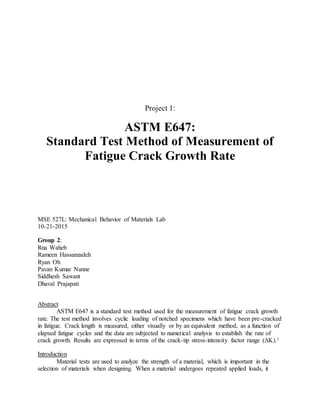
Compact tension specimen, C(T), is single edge-notch specimen designed for loads in tension. It
requires the least amount of material to evaluate crack behavior. Figure 1 shows the required
geometry for a standard C(T) specimen and figure 2 shows the notch details for the specimens.
The compact tension specimen would require a clevis and pin assembly at the top and bottom of
the specimen to allow in-plane rotation as the specimen is loaded.
.
Figure 1. Geometry of Standard C(T) Specimen

3. Figure 2. Notch Details
Grips and fixturing for the middle tension specimen M(T) depends on the width. Figure 3 shows
the required geometry for a standard M(T) specimen.
Figure 3. Geometry of Standard M(T) Specimen

4. For tension-tension loading of specimens with W ≤75 mm, a clevis and
single pin arrangement is suitable for gripping provided that the
specimen gage length is at least 3W. The gage should be at least
1.7W. For tension-tension loading of specimens with W ≥ 75 mm a
clevis with multiple bolts is recommended and the minimum specimen
gage length should be 1.5W.The specimen may also be gripped using a
clamping device instead. This type of gripping is necessary for
tension-compression loading. The minimum gage length requirement for
clamped specimens is 1.2W.
The eccentrically-loaded single edge crack tension specimen ESE(T) is similar to C(T) in its
apparatus. Figure 4 shows the required geometry for a standard eccentrically-loaded single edge
crack tension specimen.
Figure 4. Geometry of Standard ESE(T) Specimen
Good alignment is important because misalignment can cause non-symmetric cracking,
which may lead to invalid data. However, if it were to occur a strain-gaged specimen would be
useful in identifying and minimizing misalignment.
Samples do not always have to come from material with complete stress relief. The
residual stress can be minimized through careful selection of specimen shape and size.
Symmetrical specimens can also can minimize residual stress.

5. In order for results to be valid, the specimen must be predominantly elastic at all values
of applied force. There is an alternative size requirement for high-strain hardening materials.
This is done by defining replacing the yield strength with effective yield strength or flow
strength.
Using this alternative size requirement means that plastic deflections would occur in the
specimen, which could essentially double the growth rate.
The machined notch may be made by electrical-discharge machining, milling, broaching,
or sawcutting.
Table 1. Summary of Notch Preparation
EDM Mill/Broach Grind Sawcut
Notch Root
Radius
<0.25 mm <0.075 mm <0.25 mm <0.25 mm
Materials High-strength
steels
(σ≥ 1175 Mpa),
Titanium,
Aluminum
Alloys
Low/medium-
strength steels
(σ ≤ 1175 Mpa),
Aluminum
Alloys
Low/medium-
strength steels
(σ ≤ 1175 Mpa)
Aluminum Only
If residual stresses are suspected of being present, the distance between two hardness
indentations at the mouth of the notch should be measured using a mechanical gage. Data shows
that even mechanical displacement change by more than 0.05 mm can significantly change the
fatigue crack growth rates.
Once the specimen is prepped, the dimensions are measured to ensure it is within the
tolerances of its specific size. Next, it is important that it is precracked to ensure that: a) the
effect of the machined starter notch is removed from the specimen K-calibration, and 2) the
effects on subsequent crack growth rate data caused by changing crack front shape or precrack
load history is eliminated.
To test for fatigue crack growth rates above 10−8 m/cycle, it is
preferred that each
specimen be tested at a constant force range (ΔP) and a fixed set of loading variables (stress ratio
and frequency). If force range is incrementally varied it should be done so that Pmax is
increased rather than decreased to avoid delaying of growth rates caused by overload effects.

6. To test for fatigue crack growth rates below 10−8 m/cycle, start
cycling at a ΔK and Kmax level equal or greater to the terminal
precracking values. Subsequently, forces are decreased as the crack
grows and test data are recorded until the lowest ΔK or crack growth
rate of interest is achieved.
Make fatigue crack size measurements as a function of elapsed cycles by means of a
visual or equivalent technique.
Discussion
Calculations:
All calculations for desired parameters focus around Paris's Law for stress concentration,
seen below.
Here, da/dN is the crack growth rate, ΔK is the range of the stress concentration factor,
and C and m are proportionality constants that depend on the test methodology. The equation
resolves differently depending on the test type, and can be resolved through the data taken. It is
important to note that typically the regime of interest for the Paris Law is where da/dN vs ΔK is
resolvable, as seen in the center section II in the figure below.
Figure: 5 Sample plot of crack growth rate vs stress concentration range.
As noted, the paris law will be solved differently depending on the test done. For
example, for a center crack in an infinite sheet in tension, this resolves to the following:

7. Because of this, it is very important to keep in mind your test configuration while
resolving your desired parameters.
In order to solve different useful material properties, multiple methods can be used. For
example, determining the crack growth rate, da/dN, the most straightforward method is to plot
the crack length, a, vs the number of cycles, N. da/dN can then be resolved point-to-point, taking
the slope of the curve.
However, this point-to-point method has some shortcomings. Since the curve of a vs N
may be more complex. In these cases, a second order polynomial can be fit, and da/dN can be
empirically solved. This calculation method is shown below, where the regression parameters are
denoted by b.
While crack growth rate is valuable information for the current system, it is common the
consider any material that has started to crack as failed. Because of this, we can define the
parameter ΔKth as the threshold stress concentration factor. This factor is the stress concentration
range for which the crack growth rate would be sufficiently small. In the case of this paper, that
value is defined to be da/dN = 10-10m/cycle. This value is a commonly accepted “slow” crack
rate growth.
In order to solve ΔKth, a plot of log(da/dN) vs log(ΔK) should be taken. A linear regime
of this data set should be identified, ideally near the low crack growth rate regime. From this, a
linear fit, ΔK at da/dN = 10-10m/cycle can be resolved.
Conclusion
Precision and Error:
It is important to note that many sources of error can occur in these testing methods,
which in turn impact the solutions for da/dN, ΔK and ΔKth. To reduce this, it is important to
follow the guidelines for acceptable criteria and verify the data integrity as described. However,
some errors can be accounted for. For example, if the depth of the crack is shown to have
curvature, that results in more than a 5% variance in the calculation for ΔK, the curvature can be
accounted for by using a three-point through thickness measurement, measuring at the center of
the crack front, the edge of the crack front, and between these and taking the average.
Furthermore, if this curvature amount is shown to change with N, an interpolation of the
averages can be used, correcting vs two crack contours separated by at least 25% of the sample
width.

8. Figure: Illustration showing the crack front. Curvature of this front can be corrected for.
However, it is always true that not all errors can be accounted for. Therefore, it is also
important to identify the possible intrinsic variability and to determine the impact this can have
on the precision of the testing. Repeated lab testing has been done in order to estimate the impact
to precision due to different factors.
For instance, it has been shown that the amount of force applied under typical test
methods commonly has up to a 2% error. The translates proportionately to a 2% error in K, but
since da/dN can depend heavily on K, this can result in up to a 10% error.
Other sources can be more difficult to identify, so repeatability tests for variance have
been done under close-to-ideal settings. Using a highly homogenous sample in order to minimize
material errors, a variance average of 27% was found (ranging from 13-50%). Comparing lab-to-
lab in a similar method showed an average variance of 32%.
Similarly, variance in the finding of ΔKth has been explored, resulting in a 3% variance
under repeated testing in the same lab, 9% in lab-to-lab comparison. Again, do to da/dN's high
dependance on ΔK, this can result in more than an order of magnitude error in da/dN.
Furthermore, one should keep in mind that these precision findings were taken while
trying to minimize material error in the test samples. For most real samples, it is believed that
sample-to-sample inconsistencies would dominate the error. And, because there is no established
material standard for da/dN vs ΔK, it is difficult to truly determine the impact of this type of
error.
Because of this, this method should only be used when looking for gross estimates in
da/dN. When designing around these findings, one should take these errors into strong
considerations, and design in tolerances accordingly.
Reference
1. ASTM Standard E647-00, 2001 “Standard Test Method for Measurement of Fatigue
Crack Growth Rates,” ASTM International, West Conshohocken, PA,
2001.<www.astm.org>.
2. “Fatigue.” Wikipedia. Wikimedia Foundation, 19 Oct. 2015.
<https://en.wikipedia.org/wiki/Fatigue_(material)>.
3. Ali Fatemi. University of Toledo. “Fundamentals of LEFM and applications to Fatigue
Crack Growth.” https://www.efatigue.com/training/Chapter_6.pdf
4. “Mechanics of Solids.”
http://www.brown.edu/Departments/Engineering/Courses/En222//Notes/Fracturemechs/F
racturemechs.htm