Master thesis report

Max-plus to solve the job shop problem with time lags
1 | P a g e
INDEX PAGE
CHAPTER1: INTRODUCTION 3
1. Background 3
2. Problem 4
3. Purpose 5
CHAPTER2: EXTENDED BACKGROUND AND BASIC CONCEPTS 6
1. Theory 6
2. Job Shop Scheduling Problem with Time Lags 9
3. Branch and Bound concept (using partial schedules) 12
4. Cyclic (Periodical) Scheduling 12
CHAPTER 3: SYSTEM REQUIREMENTS 13
1. HOWARD Algorithm Design and Implementation 13
1. Value Determination 15
2. Policy Improvement 21
2. Modeling (Matrix A) inequalities for the sequence of operations within jobs and the
time lag constraints 26
3. Modeling second set of inequalities that forms a set of matrices iB , for i = 1 to m.
Matrices iB represents the schedule of operations on machine iM 29
4. Branch and Bound Algorithm for finding feasible B Matrices 31
CHAPTER 4: CASE STUDIES: RESULTS & COMPARISON 37
1. A (3×3) Job Sop Problems with Generic Time Lags (JSPGTL) 37
2. A (4×5) Job Sop Problems with Generic Time Lags (JSPGTL) 39
CHAPTER 5: CYCLIC JSPGTL 46
1. Suboptimal Solution: repeating the same 1 optimum cycle again and again 48
2. Improved Suboptimal Solution 48
3. Optimal Solution 53
4. Periodicity of Suboptimal Schedules 59

2 | P a g e
CHAPTER 6: CYCLIC JSPGTL: RESOURCES WITH CAPACITY GREATER THAN ONE 61
1. Case Study: A 4-sided cluster tool with wafer flow pattern 61
2. Algorithm design & implementation 63
CHAPTER 7: GENETIC ALGORITHM INTEGRATED WITH MAX PLUS ALGEBRA 67
1. Introduction 67
2. Algorithm with case study 67
 LIST OF REFERENCES 76
 LIST OF TABLES 79
 LIST OF GANTT CHARTS 80
 LIST OF FIGURES 81
APPENDIX A - DETAILED DATA REFERENCED IN THE CHAPTERS 82
APPENDIX B – SOME USEFUL MATLAB PROGRAMS 90

3 | P a g e
1. INTRODUCTION
1.1 Background
Job shop scheduling (or job-shop problem) is an optimization problem in computer science and
operation research in which ideal jobs are assigned to resources at particular times.
JSPTL is a generalization of the classical job shop problem (JSP) in which time constraints is
given, restricting the minimum or the maximum time lag between two successive operations. In
the industry this kind of problems is relatively frequent, when the process includes a thermal
treatment or a chemical treatment, the sojourn time of parts in such resources should respect a
maximal duration to prevent quality degradation. A classical example is the electroplating process
in finishing industry, where are involved operations that cannot have excessive duration in order to
maintain the quality of the products as cited in [17].
Another example concerns medical analysis where some automatic operations need to be
performed sequentially within a time window between succeeding operations because of chemical
reactions as cited in [6],[8] and [5] give some other examples of JSPTL.
This work will present a scheduling approach realized in Python(x, y) and MATLAB®
Desktop
2012b environment from scratch to tackle JSPTL problem with minimum and maximum time lags
as cited in [5],[2],[12], and [9].
In “Artigues et al., 2010”, as cited in [2] and “Lacomme et al., 2011”, as cited in [12], authors
recall a schedule can easily be obtained, taking into account the minimum time lags, but due to
maximum time lags, ’finding a non-trivial feasible schedule for the JSPTL is not simple’.
In “Lacomme et al., 2011” as cited in [12] authors study the JSP with Generic Time Lags
(JSPGTL), where time lags may link operations that belong to separate jobs.
Scheduling problems have already been tackled in the literature using max-plus algebra as
cited in [19], [4],and [3].
*** A “max-plus algebra” is a semiring over the union of real numbers and ε = , equipped
with maximum and addition as the two binary operations. A “semiring” is an algebraic
structure similar to a ring, but without the requirement that each element must have an additive
inverse. A “ring” is an algebraic structure with operations that generalize the arithmetic operations
of addition and multiplication. This will be discusses further in detail with examples in “2.1 Theory”.
In “Yurdakul and Odrey, 2004” as cited in [19], authors present a model based on a system of
non-linear max-plus equations. They propose an algorithm to solve a steady-state schedule
problem by transforming their original non-linear model into a linear one. In “Bouquard et
al.,2006” as cited in [3], authors extend the work of “Bouquard and Lent´e, 2006” as cited in [4],
that solves the two-machines flow shop scheduling problem with minimal and maximal delays: they
present results that generalize the single machine, two-machines and three-machines flow shop
scheduling problems.

4 | P a g e
A mathematical formulation for cyclic flow-shops using max-plus algebra has been presented in
“Nambiar and Judd, 2011” as cited in [14], and a method to solve the cyclic job shop scheduling
problem was proposed in “Houssin, 2011” as cited in [20].
In this manuscript we present a method based on potential inequalities and disjunctive
constraints ((“Roy and Sussman, 1964” as cited in [16]; (“Tabourier, 1969” as cited in [18]). We
propose to model the set of inequalities that define the precedence in tasks and the duration
constraints in the form of max-plus inequalities. The existence of a finite solution to such an
inequality can be effectively checked computing the so-called “spectral radius” of the
corresponding max-plus matrix, which leads to an original approach to solve the JSPTL and the
JSPGTL.
*** Spectral Radius of a Max-Plus matrix is the greatest eigenvalue of the corresponding
matrix. It will be discussed in detail in “2.1 Job Shop Scheduling Problem with Time Lags”.
Nevertheless, the set of solutions is sought within a finite (but maybe large) number of
possibilities. Our method takes advantage of the fast max-plus Howard algorithm given in “Cochet
Terrasson et al., 1998” as cited in [7]. The computation of the maximum completion time also
benefits from the max-plus model of the JSPTL that permits to eliminate a wide number of
inadequate schedules in the very first steps of our branch and-bound procedure.
*** Branch and bound procedure will be discussed in “2.2 Branch and Bound concept (using
partial schedules)”
1.2 Problem / Aim
The main focus of the thesis is to extend max plus scheduling for cyclic job shop problem. The
main idea of cyclic scheduling is to perform a set of generic tasks many times. The schedule has no
end; the same set of job is repeated one behind the other. Since most of the real life production,
manufacturing or operational cases will be of such manner e.g. Robotics where we need to repeat
same set of jobs again and again. We will consider a very-very simple example to realize the need.
Example: Suppose we have a set of four Jobs for making a bike. Each Job has a specific
purpose. Job “A” fixes all the gears on frame, Job “B” fixes the chain, Job “C” fixes the brakes and
other accessories, Job “D” fixes the rim and tire assembly. We assume this is a set of four jobs
which needs to be completed to make a bike. Now if we need to make hundred such bikes we
obviously have to repeat these set of jobs for hundred cycles, so we can easily understand the
need to extend our job shop scheduling algorithm for cyclic production.
A job may consist of a number of operations, e.g. the Job C above may consist of two
operations, one is to put brakes on frame and other is to put lights on frame which might require
one resource (machine) each. Now it is very obvious if we double the no. of resources (machines)
for each job then in one cycle instead of one bike we will now produce two bikes, so total no. of

5 | P a g e
cycles to be repeated will be fifty, now to make hundred such bikes. And this will often be the case
in real life where the no. of resources for a particular operation or for even a whole job is more
than one, so we can realize the need to formulate possible algorithm & discuss result, when using
max plus algorithm for problems with resources having capacity more than one.
Task
Extend the Jobshop problems for n cycles (n greater than one) and find
1. A schedule with completion time as minimum as possible
2. Period of the cycle.
We will perform these two tasks for following three examples
I. A (3×3) JSPGTL from Naval Industry for scheduling maintenance operations in a
shipyard.
II. A (4×5) JSPGTL the source of the problem is “A memetic algorithm for the job-shop
with time-lags”
We will also discuss and analyse the possibility of using Genetic Algorithm for finding feasible
solutions in case of a medium or big size JSPGTL where schedule is very tight and even only finding
the feasible solution is of great interest.
1.3 Purpose
Purpose of this work is to accomplish following in order to achieve our above aim.
1. We will discuss from scratch on use of max plus algebra (MPA) for scheduling of Job Shop
Problems with time lags
2. and how to extend it for cyclic job shop (CJS) problem.
3. We will also make a study on how to introduce concept of solving problems with “resources
having capacity more than one” & the future prospect of generalizing this technique for
multiple cycles for multiple resources having multiple capacities. The results for cyclic job
shop problems has already been achieved in our work but the algorithms on problems
having resource's capacity more than one for generalized case needs more work which is a
future prospect.

6 | P a g e
2. Extended Background and Basic Concepts
2.1 Theory
Max plus Algebra
Some elements on max-plus algebra are recalled in this section. More complete details on this
theory, and many applications, can be found in “Baccelli et al., 1992” as cited in [21];“Heidergott
et al., 2006” as cited in [10]; “Butkoviˇc 2010” as cited in [22].
A monoid is a set endowed with an internal operation that is associative and has an identity
element. A semiring is a set D endowed with two operations, denoted  and  , respectively called
addition and multiplication, that satisfy the following axioms.(D,  ) is a commutative monoid, (D,
 ) is a monoid, the multiplication  is distributive over finite sums (say ∀ a, b, c ∈ D,
(a  b)  c = (a  c)  (b  c), and c  (a  b) = (c  a)  (c  b)), and the neutral element of
the addition is absorbing with respect to the multiplication. The neutral element of the
multiplication is denoted e, and called unity, and the neutral element of the addition is denoted ,
and is said to be null. A dioid is a semiring (D, ,  ), with an idempotent addition, which means
that for every element x of D, the identity x ⊕ x = x holds true.
In this thesis we shall make use of the so-called max-plus algebra, that is the dioid (R ∪ {−∞},
max, +), denoted Rmax. As it is usual when dealing with Rmax, we shall in the sequel denote ⊕ the
max operation, and call it max-plus addition, and denote ⊗ the usual addition, called max-plus
multiplication. The symbol e denotes the number 0 that is the unity of max-plus addition and  is
used for −∞ that is the null element of Rmax. The latter notation is also used for a null vector, or a
null matrix, over Rmax. Finally we use the notation In for the n × n unit matrix of Rmax, and 0 is also
used for the vector which all entries equal e = 0. Another useful dioid is maxR = (R ∪ {−∞, +∞},
max, +). Any dioid D is endowed with a sup-semilattice structure, for the order defined by ∀x, y ∈
D, x ≥ y ⇔ x ⊕ y = x.
The order associated to Rmax coincides with the usual order. We also write x ≥ y for two vectors
x, y ∈ max
n
R , if xi ≥ yi, for i = 1 to n. maxR is a complete lattice for the same order, which means that
the ⊕ operation is well defined for infinite sums.
The set of square matrices over a dioid inherits the algebraic structure of dioid, with the matrix
sum and product defined as usually. The entry in position (i, j) of any matrix A is denoted, as
usually, by ijA . Over Rmax, the sum and product are then defined, for every pair of matrices A,B ∈
max
nxn
R

7 | P a g e
Definition: Sum
I. ( ) max( , )ij ij ij ij ijA B A B A B   
Definition: Product
II. (A  B) ij = 1
1
( ) max ( )
n
n
ik kj k ik kj
k
A B A B

   
Example2.1:
1 3 4
5 7 9
1 4 5
A
 
 
  
 
 
2 2 1
3 1 13
12 2 3
B
 
 
  
 
 
see I –Appendix B for max plus addition
A B 
2 3 4
5 7 13
12 4 5
 
 
 
 
 
See II –Appendix B for max plus multiplication
16 6 16
21 11 20
17 7 17
A B
 
 
   
 
 
See III –Appendix B for max plus multiplication
3
22 24 26
26 28 30
23 25 27
A
 
 
  
 
 
Definition: A matrix E ∈ max
nxn
R being given, its Kleene star, defined by
* k
k N
E E

 
is well defined on max
nxn
R . There is a max-plus spectral theory. Any square matrix E ∈ max
nxn
R admits an
eigenvalue λ, and eigenvectors x  , such that E  x

= λ  x

.
Theorem 2.1: One can show (“Baccelli et al., 1992” as cited in [21]) that the greatest eigenvalue
of matrix E, called its spectral radius, and denoted ρ (E), is equal to
III.   1/
1 1
[ ]
n
k k
ii
K i
E E
 
  

8 | P a g e
The matrix
*
E is well-defined over Rmax, with no entry equal to +∞, if and only if its spectral
radius ρ(E) is less than or equal to 0. Indeed, one can check that, if E has a strictly positive
eigenvalue λ, with eigenvector x then
k
E  x equals (k ・ λ)  x is unbounded, therefore
k
E is
unbounded, and consequently
*
E has at least one entry equal to +∞.
When
*
E is well-defined as an element of max
nxn
R , the max plus sum (III) is equal to its n first
terms. This permits to evaluate ρ (E) in finite time. When the sum does not stabilize after its n first
terms, one can deduce that ρ > 0. Finally, one can notice that, when
*
E is well-defined over Rmax,
then
*
E =
*
E  *
E , which permits to show that
*
E has a unique eigenvalue, ρ (
*
E ) = 0, and that
its Eigenvectors are the max-plus linear combinations of the columns of
*
E .
We shall consider, in the sequel, the in equation E  x ≤ x over maxR . The main results that will
be used are stated in the following theorem.
Theorem 2.2: Given a square matrix E ∈ max
nxn
R , there exists in max
n
R a finite vector x, that satisfies
the inequality E  x ≤ x, if and only if ρ (E) ≤ e.
Provided that this condition is satisfied, the least vector satisfying E ⊗ x ≤ x and x ≥ 0, is equal to
x =
*
E ⊗ 0.
Proof: We first show by recurrence that E  x ≤ x implies that
k
E  x ≤ x, for k ∈ N. This
condition is true for k = 0 and k = 1, and if it is true for k, then one has
1k
E 
 x =
k
E  E  x ≤
k
E  x ≤ x, which establishes the fact. One further deduces that
*
E  x
≤ x, and therefore that
*
E  x = x, since, by definition of the Kleene star,
*
E ≥
0
E = nI .
Now, we use the previously mentioned fact, that if ρ (E) >0, then
*
E is unbounded. In addition,
notice that
*
E  x ≤ x implies
*
( )ijE  jx ≤ ix , for every indices i, j from 1 to n.
When the indices are so that entry
*
( )ijE is equal to +∞, then either ix = +∞, or jx =  , in any
case x is not finite. This establishes the necessity of the condition.
To show the reverse, it suffices to consider the vector x that is equal to the sum of the columns
of
*
E . Provided that the condition is satisfied, this vector is finite, greater than or equal to 0, and it
is an eigenvector of
*
E , therefore satisfying the inequality E  x ≤ x, and establishing the first
statement of the theorem.
To prove the second statement we first show that for every vector b ∈ max
n
R , the product x =
*
E
 b satisfies x ≥ b, and x ≥ E  x. The latter inequality comes from the previous discussion, and
from
*
E  x =
*
E  *
E  b =
*
E  b = x. To end the proof, one can remark that any vector x
satisfying x ≥ b and x ≥ E  x also satisfies x = x  b, and x =
*
E  x, and deduce that

9 | P a g e
x =
*
E  x  *
E  b, and therefore that x ≥
*
E  b. considering b = 0 permits to end the
proof.
Remark: Theorem 2.2 actually results from a simple adaptation and concatenation of well-known
results from the literature.
For an irreducible matrix E ∈ max
nxn
R , the set  = max{ | }n
x R E x x   reduces to the null vector if
ρ (E) > e. This was first pointed out by “Gaubert, 1992” as cited in [23], and was used by “Katz,
2007, Lemma 6” as cited in [11], in the study of controlled invariance of max-plus semi modules.
The latter also used the fact, that set of solutions of x ≥ E  x is actually equal to Im
*
E . This was
first established, in the framework of minR , by “Libeaut and Loiseau, 1995”, as cited in [13],
together with the fact, that
*
E  b is the least solution of x ≥ b  E  x, for the sake of
studying the admissible initial conditions for linear systems over minR .
We did not assume that matrix E is irreducible. As we shall now see, the formulation of Theorem
2.2 is well adapted to the solution of a class of job-shop problems.
2.2 Job Shop Scheduling Problem with Time Lags
A job shop problem (JSP) is depicted by (n × m), n the number of jobs, m the number of
machines. The different jobs are denoted 1 2, ,....., nJ J J and the machines 1 2, ,....., mM M M . A job iJ
is made of a sequence of operations. Each operation is assigned to a unique machine and is not
interruptible. The sequence of operations is a priori known for each job. When more than one
operation is assigned to a machine, their execution on this machine has to be scheduled. A job
shop problem with time lags (JSPTL) consists of a JSP with additional time constraints, on the
form of time lags between pairs of operations. These delays are prescribed to stay into given time
intervals.
Time lags in a JSPTL may be maximal time lags, or minimum time lags, linking starting or
ending time of an operation with the ending or starting time of an operation within a single job. In
“Lacomme et al., 2011” as cited in [12], authors define a wider class of problems, the JSP with
Generic Time Lags. In a JSPGTL, time lags may link operations between different jobs. In the
present work, any type of time lag is considered. As a matter of fact, a set of jobs, for whose each
job has to be delivered before a given due date, is modeled as a JSPTL, each due date being a
maximum time lag between time origin and completion of the job.
Let us formalize the problem. Consider a (n × m) JSPTL, and let Ω denote the set of N
operations denoted i , for i ∈ I = {1, 2 ... N}. Let J denote the set of jobs, sI be the set of indices

10 | P a g e
of those operations that belong to job Js, for s = 1 to n, so that
ss I s   , and N = # sn
I ,
where # stands for the cardinal of a set, and k be the set of operations on machine k, Ω =
1
m
kk
 . For a given pair (i, j) of indices, we write i j  when both operations i and j
belongs to the same job, and i precedes j in its sequence. The family jI , where j = 1 to n, is a
partition of I. The notation i is used to denote the nominal duration of operation i . Finally,
min
ij
and
max
ij respectively denote the minimal time lag and the maximal time lag, between two
operations i and j subject to time constraints that may belong to the same job, in the case of a
JSPTL problem, or also belong to different jobs, in the case of JSPGTL. We call T the set of pairs of
indices (i, j) for which time constraints are defined.
The variables to be determined are the starting time of the different operations, together with
the origin, that is the starting time of the whole set of operations. We denote 0x the time origin
and ix denote the starting time of operation i . In the present study, each machine can treat a
single Operation at a time. A solution of the JSP is given by a suitable vector x that respects the
sequences of operations for each job and the capacity constraints on each machine.
The completion time for this solution is defined as
IV.
1
max( )i i
i toN
C x 

 
And a maximum completion time maxC is prescribed. One looks for an optimal solution, i.e. a vector
x that minimizes maxC , subject to:
V. maxC ≥ ix + i , ∀i ∈ I
VI. ix ≥ 0x , ∀i ∈ I
VII. jx ≥ ix + i , for i, j ∈ sI , s.t. i ≤ j, s = 1, . . . , n
VIII.
min
,j i ijx x   for i, j ∈ I,
IX.
max
,j i ijx x   for i, j ∈ I,
X. ( ) ( ),i i j i j jx x V x x     ∀ i, j ∈ kI , k = 1,. . . ,m
Inequality (V) defines the maximal completion time, (VI) states that any operation of any job
has to start after time origin, (VII) states that the order of operations in a job are a priori
determined by its sequence, (VIII) is used to express minimum time lag constraints and (IX)
maximum time lags. Inequality (X) expresses the constraint on the capacity of a machine, that

11 | P a g e
only one operation is processed at a time, i.e., for two operations i and j to be processed in the
same machine, either i terminates before j starts or the reverse holds. Inequalities (V) to (X)
can be rewritten in max-plus algebra. As long as jobs and time lag constraints are prescribed, one
can divide these inequalities into two distinct sets: A set of potential constraints corresponding to
(V-IX), that models the sequences of the jobs and the time lag constraints, and rewritten into the
form A ⊗ x ≤ x, where the matrix
( 1) ( 1)
max
N X N
A R  
 and other is a set of disjunctive inequalities (X).
max
min
max
for i = 0 and j = 1 toN
0 for i = 1 to N and j = 0
for i, j I , . , 1
for i, j
for i, j
j
j s i jij
ji
ji
C
s t s tonA
T
T

  


 
 
 
  
 
 
   
The rows and columns of matrix A are numbered from 0 to N, to take into account the variable
0x in a simple way. For the sake of simplicity, we have implicitly assumed here that no couple (i, j)
is subject to two different constraints. If it arised, one would take into account the maximal
constraint to define the corresponding coefficient ijA .
The second set of inequalities forms a set of matrices iB , for i = 1 to m. Matrices iB represents
the schedule of operations on machine iM . If im = # i denotes the number of operations to be
scheduled on this machine, the different possible schedules are in number ( im )!. Each schedule is
defined by the order of operations, say 1 2
, ......... mi i i   .
Every schedule also has to verify iB  x ≤ x, and therefore
XI. E  x ≤ x, with E =
1
m
i
i
A B

 .
A schedule is feasible if and only if the corresponding matrix E has a non-positive max-plus spectral
radius ρ (E) ≤ 0. Under this condition, the minimal nonnegative solution for this schedule is given
by
XII. minx =
*
E  0 , and
The corresponding completion time, reads minC = min
T
x   .
2.3 Branch and Bound concept (using partial schedules)
To simplify the solution, one can remark that the feasibility of partial schedules can be checked, as
well. One can as well check the feasibility of partial schedules, corresponding to matrices
i S iE A B  , for a subset S of machine indices. If the spectral radius of such a matrix is positive,

12 | P a g e
one deduces from Theorem 2.2, that, all the schedules that complete this partial schedule are not
feasible. This permits to eliminate a lot of candidates when researching a solution. Our approach
consists in using this max-plus model in a Branch and Bound like procedure. The machines are
considered one after each other. We successively compute the possible schedules for the different
machines. The existence of a solution for each partial schedule is evaluated from the computation
of the eigenvalue of partial matrices 1( )k
i iA B with k = 1, 2... m. When a partial schedule is not
feasible, we stop the examination of the corresponding branch, and when the partial schedule is
feasible, we keep it and check the following machine.
We will illustrate some case studies; these case studies used Scilab, free software for numerical
computations, and more particularly the Max-Plus toolbox, that includes fast numerical methods
like a combinatorial Howard algorithm to evaluate the max-plus spectral radius of a matrix. We will
discuss and compare our results with above.
2.4 Cyclic (Periodical) Scheduling
The main idea for such kind of problems is to perform tasks which are repeated one behind the
other. The schedules which are repeated periodically. This type of problem arises in contexts such
as robotics. We have already realized the need of it in detail via an example. We will discuss in
detail the algorithms to find a good solution and further optimize it; there is a compromise in
improving the solution and execution time.

13 | P a g e
3. System Requirements
To do the case studies and comparing result with Scilab software and it's Max-Plus tool box we
need to accomplish following :
a] Write Matlab program that models the sequences of the jobs and the time lag constraints, and
Rewritten into the form A ⊗ x ≤ x,
b] Write Matlab program that models second set of inequalities forms a set of matrices iB , for i = 1
to m. Matrices iB represents the schedule of operations on machine iM .
c] The most challenging and critical for us is to realize the HOWARD ALGORITHM in Matlab
environment, to evaluate the max-plus spectral radius of a matrix to rule out the partial schedules
that are not possible.
3.1 HOWARD: Algorithm Design and Implementation
This Algorithm is used to evaluate the max-plus spectral radius of a matrix. We are using the
algorithm presented in “NUMERICAL COMPUTATION OF SPECTRAL ELEMENTS IN MAX-PLUS
ALGEBRA” by Jean Cochet-Terrasson Guy Cohen. St´ephane Gaubert.;§ Michael Mc Gettrick . Jean-
Pierre Quadrat as cited in [7]. They describe the specialization to max-plus algebra of Howard’s
policy improvement scheme, which yields an algorithm to compute the solutions of spectral
problems in the max-plus semiring. Experimentally, the algorithm shows a remarkable (almost
linear) average execution time.
Given a matrix A ∈ max
nxn
R with at least one finite entry per row, we can compute the cycle time
vector. The cycle time vector determines the linear growth rate of the trajectories of the max plus
linear dynamical system.
There exists a close relation between max-plus algebra (and related structures) and graphs.
Consider “A” n×n matrix. The precedence graph of A, denoted by G (A), is a weighted directed
graph with vertices 1, 2, . . . , n and an arc (j, i) with weight ija for each ija  ε.
Now we can give a graph-theoretic interpretation of the max-plus-algebraic matrix power.
( )k
ijA
= 1 2 1 1 1 2 1, ......max ( )k ki i i ii i i i ja a a 
 
( )k
ijA
is the maximal weight of all paths of G (A) of length k that have j as their initial vertex and i
as their final vertex where we assume that if there does not exist a path of length k from j to i,
then the maximal weight is equal to ε by definition.
A directed graph G is called strongly connected if for any two different vertices i, j of the graph,
there exists a path from i to j. A matrix A is called irreducible if its precedence graph G (A) is
strongly connected.
If we reformulate this in the max-plus algebra then a matrix A is irreducible

14 | P a g e
If
2 3 ( 1)
( ......... )n
ijA A A A    
    for all i, j with i != j, since this condition means that for two
arbitrary vertices i and j of G (A) with i != j there exists at least one path (of length 1, 2, . . . or
n−1) from j to i
0 2
1 3 5
8 2 7
A
 
 
  
 
 
Clearly, G (A) is strongly connected, and hence A is irreducible.
(Max-plus-algebraic eigenvalue): If there exist  and v with v  1n  such that A⊗ v =  ⊗ v
then we say that  is a max-plus-algebraic eigen-value of A and that v is a corresponding max-
plus algebraic eigenvector of A. If a matrix is irreducible, it has only one eigenvalue.
Cycle mean: The mean weight of a path is defined as the sum of the weights of the individual
arcs of this path, divided by the length of this path. If such a path is a circuit one talks about the
mean weight of the circuit, or simply the cycle mean. We are interested in the maximum of these
cycle means, where the maximum is taken over all circuits in the matrix A. All circuits with a cycle
mean equal to the maximum cycle mean are called critical circuits.
If G (A) is strongly connected, there exists one and only one eigenvalue (but possibly several
eigenvectors). This eigenvalue is equal to the maximum cycle mean of the graph.
A reducible matrix A has in general several distinct Eigen values, and the maximal circuits mean
yields precisely the maximal eigenvalue.
Howard's algorithm is also known as the policy iteration algorithm, is an iterative algorithm for
computing a generalized eigenmode. First, a policy is chosen and the eigenmode of the
corresponding policy matrix is computed. This part of the overall algorithm is called value
determination and is presented in algorithmic form. Next, it is tested whether the generalized

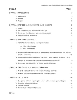
15 | P a g e
eigenmode of the policy matrix is already a generalized eigenmode of the original matrix. If so a
solution is found. If not the policy has to be adapted.
3.1.1 Value Determination
Consider a matrix A and let  be a given policy. Our aim is to compute a generalized eigenmode
of the policy matrix A
that is we wish to compute cycle time vector and Eigen vector.
The matrix A
is a bouquet matrix and the corresponding graph G ( A
) is made up of one or
more sub graphs, being sunflower graphs, with the associated matrices being sunflower matrices.
The eigenvalue of a sunflower matrix exists and equals the mean of only circuit in the associated
sunflower graph. A corresponding eigenvector follows by going along the circuit and paths, starting
from an arbitrary chosen node in the circuit.
Sunflower Graph: Sunflower has only one circuit associated with it.
2
1 5
7
S
 
 
 
 
 
  
 
 
Figure1 shows a sunflower graph with entries corresponding to matrix S1.
Figure1: Sunflower Graph S1
Cycle time vector = (5 + 2)/ 2=3.5
Another sunflower graph
7
2 4
3
S
 
 
 
 
 
  
 
 
Cycle time vector = (7 + 4 + 3)/ 3
=4.667

16 | P a g e
Figure 2 shows a sunflower graph with entries corresponding to matrix S2.
Figure 2: Sunflower Graph S2
A bouquet graph is a collection of various such sunflower graphs. An example of a bouquet graph is
shown below in Figure 3.
Figure 3:Bouquet Graph
This is a bouquet graph and the matrix associated with it will be bouquet matrix. For each obtained
eigenmode, the cycle time vector  will be unique, whereas the vector  will not be unique. How
the vector  is calculated will be shown next.
Choosing the initial policy A
in fact is choosing a bouquet matrix which may be a collection of
several sunflower graphs.
Now we will discuss how we realized the algorithm in program for finding the bouquet matrix.
We will take the following small example for illustration

17 | P a g e
1 2 7
3 5
4 3
2 8
A

 
 
 
 
 
 
 
 
 
We have to find the cycle time vector and the eigen vector for this given matrix using the Howard
Algorithm i.e. the value determination and the policy improvement.
Recalling the above example of sunflower graph again
7
2 4
3
S
 
 
 
 
 
  
 
 
The Sunflower graph corresponding to S2 is shown in figure 4.
Figure 4: Sunflower Graph S2
Entry S21 in the communication graph means the arc is directed from 1 towards 2, similarly S32
means the arc is directed from 2 towards 3. Now, returning back to our original matrix A. The
howard algorithm is realized via the main Matlab program “HowardA.m” see [4]- Appendix B. The
input to the program is simply the matrix A for which we need to find the cycle time vector and
Eigen vector, which in our case will be A B . There are 12 subroutines in this program listed in
appendix B (see [5]-[16], Appendix B). We will now go through the programs in brief to
understand how the algorithm is realized.
The subroutines Cmat, compbouq, inipolicy, allloop and sunflower are programmed for finding
the initial policy (bouquet curve).
The first subroutine in the program is “Cmat”. This gives us the indices of the finite entries of
the matrix in the given format. There are 2 outputs of this subroutine new
C & scl, scl gives the finite

18 | P a g e
diagonal entries and
new
C gives other finite entries in the matrix. Each column of the
new
C matrix
represents the index of the finite entry of the matrix A.
1 1 2 3 3 4 4
2 4 3 2 4 2 3new
C
 
  
 
i.e A12, A14, A23, A32, A34, A42, A43 is the finite entries of the matrix A. A12 represents that arc is
directed from 2 towards 1.
 1 3 0 0scl 
i.e. A11 and A33 are self closing loops or the diagonal entries.
The following characteristics of the bouquet and sunflower matrix will be very helpful in
understanding the algorithm further.
1. The sunflower graph should only consist of one closed loop.
2. The bouquet graph can consist of more than one loop.
3. Each finite element of the matrix “A” need to be associated with at least one arc.
4. Only the nodes contained by the loops of the bouquet graph have two associated arc.
5. Each node of the bouquet graph should precisely have one incoming arc except the nodes of
the loop as mentioned in the previous point.
6. The outgoing arcs can be more than one but incoming arc is precisely one.
7. No node can be a part of more than one closing loop.
Next subroutine is “sunflower.m” for randomly finding a close loop which is the first step in finding
a sunflower graph and ultimately the bouquet matrix. Some of the features in achieving this
objective are listed below.
With some lines of code we try to rearrange the new
C in the following form
4 3 2 3 4 1 1
3 2 3 4 2 4 2
C
 
  
 
The peculiarity of this form is entry of the second row of first column is same as first row of next
column. How this form is helpful in finding a close loop can be easily realized, when we plot the
graph of Matrix “A” corresponding to the indices of first five columns.

19 | P a g e
Figure 5: Communication Graph Matrix A
We can see by extracting the first five columns of “C” and plotting them we found a graph with
two closed loops, which very roughly fulfils our motive for this subroutine. But this is not a bouquet
matrix as node 3 is contained by two closed loops.
After some manipulations we will reduce it to finding a close loop which is denoted by “D” in our
Matlab program. D obtained in our present example will be
3 2
2 3
D
 
  
 
But the program is totally random, if in the given
1 1 2 3 3 4 4
2 4 3 2 4 2 3new
C
 
  
 
the algorithm does not find a close loop it will randomly choose two columns in newC and swap
them, this happens for three-four cycles until we find a close loop and if it does not find a close
loop then the algorithm selects self closing loop such as A11 or A12 etc as “D”.
Next task is to find the sunflower graph that is we will randomly select a random node from the
close loop “D” and try to visit the nodes as many as possible. We have “sunflower.m” subroutine
for this purpose (see [8]- Appendix B). This subroutine has three outputs represented as “D, E &
EN” D represents closed loop, E represents the randomly chosen node and EN represents the
number of nodes contained by the close loop. We already have a close loop “D” to start with, in our
search for sunflower graph. But all the nodes in a sunflower graph needs to be visited exactly once
so all the entries in first row of newC with these needs need to be deleted, as we do not wish visit
them again.
So our new “C” is
4 4 1 1
3 2 4 4
aC
 
  
 

20 | P a g e
So we will keep modifying our “C” as we keep visiting more and more nodes for finding our
sunflower graph. Now we will take a bigger example to understand the algorithm further which is
not possible by this small example.
Example 3.1: Consider matrix A of size (21 X 21) – for detailed data (see [1]- Appendix A)
As above example this gives us newC which contains the indices of finite entries of the matrix as
discussed before, for detailed data (see [2]- Appendix A). The above “A” matrix is basically taken
from a case study (4 x 5 JSPGTL).
*** We know the “A” matrix models the sequences of the jobs and the time lag constraints. If
we see the meaning of the entries in first column of A, it represents the minimum time lag with
respect to the origin, and this value will always be greater or equal to 0. So, we can always be sure
that the entries in the first column will be finite.
For making our “Howard Algorithm” realization faster we can use a small trick based on our
above mentioned fact for finding the initial bouquet graph (initial policy) i.e. we can start with an
initial sunflower graph having close loop
1
1
 
 
 
.
Figure 6: Initial Sunflower Graph 4 x 5 JSPGTL
Now we will try to visit the remaining nodes. We will delete all the column entries having node 1
in first row as we do not want to travel to node 1 again because it will not be a bouquet graph
then. So new newC matrix obtained after this will be “Ca” (size 2x 52), see [3]- Appendix A.
Now keeping in mind basic concept of bouquet graph stated earlier we will try to visit as many
nodes we can from node 1 and will denote the corresponding matrix containing all these arcs by
“vectr”.
vectr=
2 3 4 5 6 7 8 9 10 11
1 1 1 1 1 1 1 1 1 1



12 13 14 15 16 17 18 19 20 21
1 1 1 1 1 1 1 1 1 1



The columns
represent corresponding arcs e.g. the first column entry
2
1
 
 
 
represents an arc from node 1 to node

21 | P a g e
2. Since all the remaining nodes are visited at once by node 1, the new “Ca” matrix will be empty
and we can choose the following as initial policy.
A
=
1
1



2 3 4 5 6 7 8 9 10 1112 13 14 15 16 17 18 19 20 21
1 1 1 1 1 1 1 1 1 1 1 1 1 1 1 1 1 1 1 1



The communication graph is shown in figure 7.
Figure 7 : Communication Graph: Initial Policy
This graph is an example of a sunflower graph with self close loop. This is a very special case as
our sunflower graph is turned out to be a bouquet graph.
A
is the Initial policy. Next step in the Algorithm is to calculate the cycle time vector and the
Eigen vector for the policy i.e. computing a generalized eigenmode. The maximum cycle vector is
the Eigen value of the matrix. Cycle time vector is the average weighted mean of the close loop,
which is 0/1=0 in this case.
Now we will check if it’s the generalized Eigen mode of the given matrix i.e. this is the
maximum cycle vector possible among any possible policy. If it is not then we will have to choose a
new policy which will be an improvement in the earlier policy. This will be illustrated in Step 2-
Policy Improvement of the Howard Algorithm. “ ” is cycle time vector.
3.1.2 Policy Improvement: Now we have two steps to follow:
1. Determine the set 1I =
( , ) ( )
{ ( ) | max }i j
j i D A
i N A  

  .

22 | P a g e
 If 1I = , then compute D (A*) = {(j, i)   }
i j
D A  
 and continue with step 2.
 If 1I  , then determine all i ∈ 1I the sets
 
1
i
D A = {(k, i) ∈ D (A) |
( , ) ( )
max }k j
j i D A
 


Define a new policy
'
 as
'
i : =
    1
1
_ _ 1
, , ( )i
i
k i for some k i D A if i I
if i I
   
 
  
2. Determine the set
*
2
( , ) ( )
( ) | max( )i ij j j
j i D A
I i N A v a v 

  
    
  
.
 If 2I = , then the current “ ” and “V” are general Eigen modes and satisfies the
requirement. Hence the algorithm can stop.
 If 2I  , then determine for all i ∈ 2I the sets
          , *
2
( )= | ( }, .ik k k j i ij jD Ai jD A k i D A v max va a      
Define a new policy
''
i as
''
i =
     
2
2
_ 2
, ,
_
i
i
if i I
  
 
 
 

The function “eigenvec.m” calculates the generalized Eigen vector of the policy (See [10], Appendix
B).
Calculating 1I
1I =
( , ) ( )
{ ( ) | max }i j
j i D A
i N A  

 
We will get 1I = , since 1I is null we will proceed with step 2 and calculate 2I
Say E= D (A*) = {(j, i)   }
i j
D A  

We get E= [2 3 4 5 6 7 8 9 1110 12 13 14 15 16 17 18 19 20 21 22 1]
*
( , ) ( )
1 ij j j
j i D A
WP a v 

  (See[4], Appendix A)
*
2
( , ) ( )
( ) | max( )i ij j j
j i D A
I i N A v a v 

  
    
  

23 | P a g e
We get 2I
 3 4 5 6 8 9 10 11 13 14 15 16 18 19 20 21
Since 2I  , we calculate
''
i =
     
2
2
_ 2
, ,
_
i
i
if i I
  
 
 
 

'
i for 2i I is denoted by “ImpPol”
ImpPol=
3 4 5 6 8 9 10 11 13 14 15 16 18 19 20 21
2 3 4 5 7 8 9 10 12 13 14 15 17 18 19 20
 
 
 
We will make these changes in the new policy. We will keep repeating the above process until
we have reached to condition 2I  , then this algorithm can be terminated.
Final bouquet graph will be given by “circ”
Circ=
6 11 16 21 5 10 15 20 4 9 14 19 3 8 13 18 2 7 12 17 1
5 10 15 20 4 9 14 19 3 8 13 18 2 7 12 17 1 1 1 1 1
 
 
 
The corresponding generalized Eigen vector will be given by “eigv”
 320 127 184 158 254 88 87 124 159 40 66 78 72 5 46 59 0 0 0 0 0
And the cycle time vector  will be 0.
We will consider another small example which has more than one sunflower graph.
Example 3.2 A=
6 2 inf 7
inf 3 5 inf
inf 4 inf 3
inf 2 8 inf
 
   
  
 
  
The closed loop we get by our program is
2 3
3 2
D
 
  
 
Initial policy A
is represented by “GP” in our program
GP =
1 4 2 3
2 3 3 2
 
 
 
Cycle time vector is represented by “Netavec” in our program
Netavec= = [4.5000 4.5000 4.5000 4.5000]
Generalized eigenvector v= [-2.5000 0 -0.5000 3.0000]
We will get 1I 
2 [1 3 0 0]I 

24 | P a g e
Since 2I  , Improvement in policy is required
ImpPol
1 3
4 4
 
  
 
New Improved Policy
'
A
will be given by GP’
GP’=
2 1 4 3
3 4 3 4
 
  
 
Now we will follow all the steps again, we will get new
Netavec=  5.5 5.5 5.5 5.5
New Generalized Eigen vector
V  4.5 0 .5 3
Further we get 2 1I  , so improvement in policy is required
ImpPol=
1
1
 
 
 
New policy after improvement is GP” =
''
A
=
2 3 4 1
3 4 3 1
 
 
 
Netavec=  =  6 5.5 5.5 5.5
New generalized Eigen Vector will be  4.5 0 .5 3v 
Now 1 2I I  
We have maximum cycle time vector  =6 for sunflower graph containing only node 1. Now we
will try to find the maximum cycle time vector for remaining of the bouquet matrix.
Remaining bouquet matrix is
2 3 4
3 4 3
 
 
 
Netavec= = [5.5000 5.5000 5.5000]
Generalized Eigen Vector will be  0.5 0 2.5v  
1 2I I   , so the algorithm can be terminated.

25 | P a g e
Hence, final Netavec is  6 5.5 5.5 5.5 
& Eigen vector is  4.5 0 .5 3v 
We, will consider one more example
Example 3.3:
2 1 0 1 1
inf 2 4 inf inf
inf 4 1 inf inf
inf inf inf 2 inf
5 0 inf 0 2
 
    
   
 
    
  
Close loop found by our program
D=
2 3
3 2
 
 
 
The associated sunflower graph will be
5 1 2 3
2 3 3 2
 
 
 
Since matrix A has 5 nodes and all nodes are not covered by this sunflower graph the function will
be made to run again but deleting the nodes already covered, the only node left is node 4 so in
next cycle the loop (4, 4) will be added to this to make it a bouquet graph.
New bouquet matrix will be
4 5 1 2 3
4 2 3 3 2
 
 
 
We get Netavec =  = 4 4 4 2 4
Eigen Vector=  4 0 0 0 4v   
We calculate  5 1 2 3 0E 
&  2 5 1 0 0 0I  , since 2I 0 we have an improvement in policy
ImpPol=
5 1
1 2
 
 
 
New Improved policy is GP’=
'
A
=
5 1 2 3 4
1 2 3 2 4
 
 
 

26 | P a g e
Netavec=  = 4 4 4 2 4
V=  3 0 0 0 2 
Since 1 2I I   , the algorithm can be terminated
Maximum cycle time vector is 4 for the sunflower graph
5 1 2 3
1 2 3 2
 
 
 
and
The other sunflower graph will be
4
4
 
 
 
So the generalized eigen mode for the bouquet matrix will be  = 4 4 4 2 4 &
v = 3 0 0 0 2 
*** This is the algorithm we used to realize Howard algorithm via Matlab and python program.
The algorithm gave correct results for all the case studies and examples that we run and included
in this thesis but the execution time in calculating the generalized eigen mode of a given matrix by
this algorithm on comparison with “Scicos Lab” max plus tool box for howard algorithm is quite
significant and this is the only drawback we have, which we will try to improve later, this is beyond
the scope of this master thesis.
3.2 Modeling the sequence of operations within jobs and the time lag
constraints, and rewrite into the form A ⊗ x ≤ x
To explain 3.2 and 3.3 we will take a case study: A (3×3) JSPGTL
The following table gives the machine number and duration for the operations of the jobs.
1 2 3
1 1 2 3
2 1 3 2
3 3 1 2
( ,10) ( ,35) ( ,35)
( ,15) ( ,16) ( ,12)
( ,11) ( ,12) ( ,21)
O O O
J M M M
J M M M
J M M M
 
 
 
 
 
 
J- Job, O- Operation, M- Machine
Further time lag constraints have to be taken into account:

27 | P a g e
• A minimum time lag of 20 must occur between the end of the first operation of 1J and the
beginning of the second operation of 2J ;
• Between both previous events, there is a maximum time lag of 30;
beginning of the first operation of 3J ;
ix Denotes the starting time of “ith
” operation and i denotes the processing time of the “ith
”
operation, therefore above constraints can be expressed by following equations
mint = min time lag | maxt= max time lag.
1 1x  + mint  5x
i.e. 1x + 10 + 20<= 5x | 1x + 30 <= 5x
1 1x  + maxt >= 5x
i.e. 1x + 10 + 30>= 5x | 1x +40 >= 5x Similarly other constraints
4x + 4 + mint<= 7x
i.e. 4x + 15 + 5<= 7x | 4x + 20 <= 7x
4x + 4 + maxt >= 7x
i.e. 1x + 15 + 20>= 5x | 1x +35 >= 5x
For programs see [17]-[20] Appendix B for the formulation A, B matrices and obtaining the
solution (Optimum Schedule). We will store constraints in a different matrix named as “LAG”, and
the sequence of operations will be stored in matrix A and the final matrix A will be
A = A ⊕ LAG
The LAG Matrix because of above constraints is shown in next page.

28 | P a g e
LAG=
-Inf -Inf -Inf -Inf -Inf -Inf -Inf -Inf -Inf -Inf
-Inf -Inf -Inf -Inf -Inf -40 -Inf -Inf -Inf -Inf
-Inf -Inf -Inf -Inf -Inf -Inf -Inf -35 -Inf -Inf
-Inf 30 -Inf -Inf -Inf -Inf -Inf -Inf -Inf -Inf
-Inf -Inf -Inf -Inf 20 -Inf -Inf -Inf -Inf -Inf











 
 
 
 
 
 
 
 
 
 
The operations of a job can be formulated similarly
e.g. for Job 1J
1x + 1 >= 2x
2x + 2 >= 3x
Similarly for Job 2J and Job 3J
4x + 4 >= 5x 5x + 5 >= 6x
7x + 7 >= 8x
8x + 8 >= 9x
Matrix “A” will look like this
0 inf inf inf inf inf inf inf inf inf
0 0 inf inf inf inf inf inf inf inf
0 10 0 inf inf inf inf inf inf inf
0 inf 35 0 inf inf inf inf inf inf
0 inf inf inf 0 inf inf inf inf inf
0 inf inf inf 15 0 inf inf inf in
        
       
      
      
       
       f
0 inf inf inf inf 16 0 inf inf inf
0 inf inf inf inf inf inf 0 inf inf
0 inf inf inf inf inf inf 11 0 inf
0 inf inf inf inf inf inf inf 12 0
 
 
 
 
 
 
 
 
 
       
 
        
       
 
        

29 | P a g e
( A LAG ) Will be
0 0 inf inf inf 40 inf inf inf inf
0 inf inf inf 0 inf inf 35 inf inf
0 30 inf inf 15 0 inf inf inf inf
0 i
        
       
      
      
       
     
 nf inf inf inf 16 0 inf inf inf
 
 
 
 
 
 
 
 
 
      
 
       
       
 
        
3.3 Modeling second set of inequalities forms a set of matrices iB , for i = 1 to m. Matrices
iB represents the schedule of operations on machine iM . Considering same example
1 2 3
1 1 2 3
2 1 3 2
3 3 1 2
( ,10) ( ,35) ( ,35)
( ,15) ( ,16) ( ,12)
( ,11) ( ,12) ( ,21)
O O O
J M M M
J M M M
J M M M
 
 
 
 
 
 
The processing time for the corresponding operations in our Matlab program is defined as
CT=
10 35 35
15 16 12
11 12 21
 
 
 
  
1 4 8
2 6 9
3 5 7
Iindex
 
   
  
The rows of the Iindex represents the machine i.e. row one for machine 1M , row two for machine
2M and so on.
The Iindex tells about the corresponding operation on the machine.
e.g. row one [ 1 4 8] tells - On machine 1M , operations “1” ,”4” and “8” will be performed.
Row two [2 6 9] represents - On machine 2M , operations “2” ,”6” and “9” will be performed.

30 | P a g e
‘T1’ represents the processing time corresponding to Iindex.
10 15 12
1 35 12 21
35 16 11
T
 
   
  
Total no. of possible sequences of operations will be 3! =6
8 <4 <1
8 <1 <4
4 <8 <1
4 <1 <8
1 <4 <8
1< 8< 4
So we will have six “B” matrices for Machine 1M and similarly for other two machines.
The formulation of B matrix for the sequence [1 < 4 < 8] on machine 1M
1 1 4x x 
4x + 4 8x
1x + 1 8x
 1 4 8
B  
=
inf inf inf inf inf inf inf inf inf inf
inf 10 inf inf inf inf inf inf inf inf
i
         
         
         
         
        
 nf inf inf inf inf inf inf inf inf inf
inf 10 inf inf 15 inf inf inf inf inf





        
         
         
       
         





 
 
 
 
 
 
 
 
 
 
Similarly, for other 5 sequences [8 < 4 <1], [4 <1 <8] etc. B matrix can be calculated. Similarly
there will be six possible B matrices for every machine.
This is the exhaustive way of calculation, where we calculate all the possible sequences of B
matrix.

31 | P a g e
3.4 Branch and Bound Algorithm for finding feasible B Matrices
Hence one can as well check the feasibility of partial schedules, corresponding to matrices E =
iA B for a subset S of machine indices. If the spectral radius of such a matrix is positive, one
deduces from Proposition, that, all the schedules that complete this partial schedule are not
feasible. This permits to eliminate a lot of candidates when researching a solution. Our approach
consists in using this max-plus model in a Branch and Bound like procedure. The machines are
considered one after each other. We successively compute the possible schedules for the different
machines.
The existence of a solution for each partial schedule is evaluated from the computation of the
eigenvalue of partial matrices ( iA B ). When a partial schedule is not feasible, we stop the
examination of the corresponding branch, and when the partial schedule is feasible, we keep it and
check the following machine.
We will solve the above problem by this technique
For Machine 1M , the set of operations are [1 4 8]
We will start with the subset [1 8] of the operation, for this possible sequences will be 2! =2
V1 =
8 1
1 8
 
 
 
We will calculate | 1,2iA B i  , and calculate spectral radius for all i.
Matrix corresponding to value i=1 is shown below.
1A B =
0 0 inf inf inf 40 inf inf 12 inf
0 inf
        
      
      
      
       
     
 inf inf inf 16 0 inf inf inf
 
 
 
 
 
 
 
 
 
      
 
       
       
 
        
Cycle Time Vector =  = 0

32 | P a g e
Eigen Vector= [88 89 53 73 43 43 31 20 0 0 ]
Bouquet matrix is represented by Circ=
4 7 3 6 2 10 9 8 5 1
3 6 2 2 9 9 8 5 1 1
 
 
 
Since  = 0, so this is a good sequence, Now we calculate 2A B
2A B =
0 0 inf inf inf 40 inf inf inf inf
0 i
        
       
      
      
       
     
 nf inf inf inf 16 0 inf inf inf
0 10 inf inf inf inf inf 11 0 inf
 
 
 
 
 
 
 
 
 
      
 
       
      
 
        
Cycle time vector or spectral radius =0
Eigen vector = [43 45 46 31 10 30 20 0 0 0]
circ=
10 4 7 9 3 6 8 2 5 1
9 3 6 8 2 2 5 1 1 1
 
 
 
So the subset sequence [8<1] needs to be continued with other operation to check feasibility. On
combining third operation “4” on this particular machine we will have six possible B matrices as
before.
***: The process of selecting the partial schedule or selecting the subset of indices of operations
of a machine is random meaning out of [1 4 8] every time we run the operation the possible set of
two operation can be [1 4], [4 8], [1 8] any, So in this case for this small problem we didn't gain
any benefit by our branch and bound method.
So let us try to run the program again
8 4
1
4 8
V
 
  
 
1 (8 4)|A B  See [5]-Appendix A for detail data.
Cycle time vector
 0 14.3333 14.3333 14.3333 14.3333 14.3333 14.3333 14.3333 14.3333 14.3333 
Since maximum cycle time vector is positive we don't have a good sequence, all possible
sequences with this subsequence will be non feasible. The corresponding bouquet matrix is

33 | P a g e
circ=
1 4 3 10 2 7 6 5 9 8
1 3 2 9 6 6 5 9 8 5
 
 
 
This bouquet matrix has two sunflower graphs
1
1
 
 
 
&
4 3 10 2 7 6 5 9 8
3 2 9 6 6 5 9 8 5
 
 
 
Sunflower graph 1, with close loop node 1 is shown in Figure 8.
Figure 8 : Sunflower graph 1
Sunflower graph 2, with close loop node 5, 9 and 8 is shown in Figure 9.
Figure 9: Sunflower graph 2
Now we calculate 2 4 8|A B  see [6]- Appendix A
Cycle time vector= 0 
Eigen Vector= Eigv= [43 45 46 31 10 30 20 0 0 0]

34 | P a g e
Bouquet Matrix is
10 4 7 9 3 6 8 2 5 1
9 3 6 8 2 2 5 1 1 1
 
 
 
Since [4<8] is the only good subsequence to carry on, therefore we have an advantage here
because in the next step we combine this sequence with [1] and all possible combination generated
will be three so instead of six , we need only to calculate spectral radius of three matrices.Three
possible sequences are represented by V1
V1=
1 4 8
4 1 8
4 8 1
 
 
 
  
I. Now we calculate 1 (1 4 8)|A B   see [7] Appendix A.
Since, Cycle time vector= 0  , this is a good sequence.
Eigen Vector= Eigv= 53 41 45 30 46 10 10 30 0
Bouquet matrix =circ=
10 9 4 8 7 3 5 6 2 1
9 8 3 5 6 2 2 2 1 1
 
 
 
II. Now we calculate 2 (4 1 8)|A B   see [8] Appendix A.
Cycle time vector= 0  , this is a good sequence
Eigen Vector= Eigv= 60 61 43 25 45 3115 20 0 0
Bouquet matrix =circ=
4 7 10 3 6 9 2 8 5 1
3 6 9 2 2 8 5 5 1 1
 
 
 
III. Now we calculate 2 (4 8 1)|A B   see [9] Appendix A.
Cycle time vector= 0  , this is a good sequence
Eigen Vector= Eigv= [88 89 53 73 43 43 31 20 0 0]
circ=
4 7 3 6 10 2 9 8 5 1
3 6 2 2 9 9 8 5 1 1
 
 
 

35 | P a g e
So all these sequences are good for machine 1M and represented by V1=
1 4 8
4 1 8
4 8 1
 
 
 
 
 
For Machine 2 similarly, we get six good sequences which mean all possible sequences are good.
6 9 2
9 6 2
 
 
 
9 2 6
6 2 9
2 6 9
2 9 6
 
 
 
 
 
 
For Machine 3 similarly, we get two good sequences.
5 7 3
7 5 3
 
 
 
Now at next step we will combine all these sequences of different machines to find good
sequences, stepwise.
First we try to find feasible sequences among all possible sequences of Machine 1 and Machine
2 when combined. Machine 1 has three and Machine 2 has six sequences so combining these will
give a possible of 3 x 6= 18 sequences represented by “gooseq” (See [10] Appendix A).
1 3 1 6( | ) ( | )i i j jC A B A B      
“ceig” is the array where we stored maximum cycle vector of all the possible 18 sequences
ceig =[ 0 0 0 0 0 0 0 0 0 0 0 0 0 0 0 0 0 0]
Since all the maximum cycle time vectors are zero, so all sequences are good.
Now we will combine the result of these two machines with the last third machine i.e. we calculate
1 18 1 2( | ) ( | )i i j jD C A B      After combining these three machines we will get eighteen good
sequences (see [11] Appendix B).
From formula XII, Page 11 we know that a schedule is feasible if and only if the corresponding
matrix E (E =
1
m
i
i
A B

 ) has a non-positive max-plus spectral radius ρ (E) ≤ 0. Under this condition,
the minimal nonnegative solution for this schedule is given by minx =
*
E  0.
We will obtain 18 sets of minx one for each schedule, contained in the matrix ‘COT’=
1 2 3 18min min min minx x x .........x  

36 | P a g e
Vector minx represents the optimal starting time for each operation.
The corresponding completion time, reads minC = minx   .
We will obtain eighteen sets of minC one for each schedule, contained in the matrix ‘DOT’=
1 2 3 18min min min min.........C C C C  
Optimum minx = [0 10 57 11 30 46 46 57 69]
Optimum minC = [10 45 92 26 46 58 57 69 90]
Minimum completion time = Max (Optimum minC ) = 92
*** In Chapter three we learnt how to model constraints, operation sequences within a job,
constraints considering the capacity of a machine, how to use branch and bound technique to
obtain feasible solutions and solve for optimum minx and minC . We will use these algorithms and
information in Chapter four for two case studies.

37 | P a g e
4. CASE STUDIES:
4.1 A (3×3) JSPGTL:
We already discussed this case study for illustrating the design of algorithm in 3.2 and 3.3.
This Problem was taken from Lacomme et al., 2011 (as cited in [12]). The second problem is a
medium size problem that comes from the naval industry. It tackles the problem of scheduling the
maintenance operations in a shipyard. A first study based on Supervisory Control Theory of Timed
Discrete Events has been presented in Pinha et al., 2011 (as cited in [15]). The following table
gives the machine number and duration for the operations of the jobs.
1 2 3
1 1 2 3
2 1 3 2
3 3 1 2
( ,10) ( ,35) ( ,35)
( ,15) ( ,16) ( ,12)
( ,11) ( ,12) ( ,21)
O O O
J M M M
J M M M
J M M M
 
 
 
 
 
 
J- Job, O- Operation, M- Machine
Further time lag constraints have to be taken into account:
beginning of the second operation of 2J ;
beginning of the first operation of 3J ;
Table 1: 3 x 3 JSPGTL
JOB SHOP PROBLEM
Machines Operations
Optimal Starting
Time1
Processing
Time
Completion
Time
Machine1
Operation 1 0 10 10
Operation 4 11 15 26
Machine2
Machine3 Operation 3 57 35 92

38 | P a g e
Gantt Chart 1: 3 x 3 JSPGTL
Above is the Gantt chart 1 for the problem, the bar in blue indicates the optimal starting time i.e.
the corresponding operation can only start after this due to constraint or because the machine is
not free. As we can see in the chart, operation 7 starts just after operation 5 is finished. Operation
3 starts just after operation 7 is finished and machine gets free. But we can easily see on chart
there is a huge waiting time (blue bar) between the end of operation 4 and starting of operation 5
and during this time the machine is idle, machine is free but not utilized, this is because of the
constraints. The Optimal Completion time for complete set of jobs is “92” which corresponds to
Operation 3 scheduled on machine 3.
0 20 40 60 80 100
O1
O4
O8
O2
O6
O9
O3
O5
O7Machine1Machine2Machine3
OST1
PT
0 20 40 60 80 100
O1
O4
O8
O2
O6
O9
O3
O5
O7
Machine1Machine2Machine3
OST1
CYC1

39 | P a g e
4.2 A (4×5) JSPGTL
The source of the problem is “A memetic algorithm for the job-shop with time-lags” by “Anthony et
al., 2008” as cited in [24].
A job-shop problem with minimal and maximal delays between starting times of operations. In
the article, time-lags between successive operations of the same job are studied. This problem is a
generalization of the job-shop problem (null minimal time-lags and infinite maximal time-lags) and
the no-wait job-shop problem (null minimal and maximal time-lags). They used in the article a
framework based on a disjunctive graph to model the problem and on a memetic algorithm for job
sequence generation on machines. We will schedule this problem with the max plus algebra
inequality.
Problem consists in finding a feasible schedule that is, an allocation of the operations to
machine time intervals, which has minimal length.
(Problem consists of four jobs, five machines):
72 5 46 59
87 35 20 19
95 48 21 46
66 39 97 34
60 54 55 37
D
 
 
 
 
 
 
  
Matrix D indicates duration of operations, first row indicates first operations of each job and
column indicates the number of jobs, this is the standard form of input in ScicosLab max plus.
2 5 2 1
1 4 4 4
5 1 3 5
3 3 1 2
4 2 5 3
R
 
 
 
 
 
 
  
Indicates the resource / machine used
TT= [380,181,239,195]
DT= 5*TT; DT is due time for each job.
max
0 0 0 0
0 0 0 0
0 0 0 0
0 0 0 0
0 0 0 0
D
 
 
 
 
 
 
  
maxD Indicates the max. time lag

40 | P a g e
Additional constraints
Case 1: No waiting time: Once operation is done, the part must move for next operation w/o
waiting
Case 2: No additional constraints
Solution: Case 1
72 87 95 66 60
5 35 48 39 54
46 20 21 97 55
59 19 46 34 37
CT
 
 
 
 
 
 
This is the format of our Algorithm. CT is the matrix with processing times, rows indicates the jobs
1 2 3 4, , &J J J J from top to down, and operations 1-5 from left to right.
1 11 19 10
6 3 18 15
16 2 8 14
7 12 17 5
13 4 9 20
Iindex
 
 
 
 
 
 
  
“Iindex” rows correspond to machine 1M - 5M from top to bottom, and elements give the index
of operation e.g. the first row second entry is 11, this means on machine 1M after first operation,
the operation eleven will come for processing.
72 46 34 54
5 95 46 55
1 59 87 48 97
35 20 19 60
21 66 39 37
T
 
 
 
 
 
 
  
T1 contains processing time corresponding to Iindex.
A is a 21x21 matrix (see [1]- Appendix A) we can see A (3, 2) = - A (2, 3) = 72
This means there is no waiting time, as soon as operation one finishes operation two starts.
Similar to A, LAG will be a 21x21 matrix
Except the following entries which correspond to due time, all other entries will be –inf.
LAG (1, 6) =-5*380+60; LAG (1, 11) =-5 *181+54;
LAG (1, 16) =-5 *239+55; LAG (1, 21) =-5 *195+37;
Cycle time vector= 0 
eigv= [320 127 184 158 254 88 87 124 159 40 66 78 72 5 46 59 0
0 0 0 0]

41 | P a g e
For each machine there are 4! = 24 possible schedules, and in this case we have obtained that all
24 schedules are feasible for each machine.
At next step we will combine all the five machines one by one at each step.
 We will combine machine 1M and machine 2M
Let 1 1 24|i iB   represents schedules on machine 1M and
2 1 24|i iB   Represents schedules on machine 2M
We will try to find all possible combinations of  1 1 24 2 1 24( | ) ( | )i ji jA B A B      and check if
they are feasible. There will be a total of 24x24 =576 possible combinations to check for. Out of
these only 89 are feasible. These 89 feasible schedules are stored in vector C.
 Now at next step we will further combine machine 3M
 1 89 3 1 24( | ) ( | )ji i jC A B    
It will produce a total of 94 feasible schedules out of total 89 x24 = 2136 possible schedules.
All these 94 schedules are stored in vector D
 at next step we will further combine machine 4M
 1 94 4 1 24( | ) ( | )ji i jD A B    
This yields a total of 163 feasible solutions out of total possible 94 x 24 = 2256 schedules.
All these 163 feasible solutions are stored in matrix E
 at last step we will further combine machine 5M
 1 163 5 1 24( | ) ( | )ji i jE A B    
The total possible sequences in this will be 163 x 24 = 3912. Finally we get 169 feasible schedules
and we have to choose an optimum schedule among them.
Results are shown below in tabular form in table 2
OST- Optimal Starting Time | PT – Processing Time | CT – Completion Time
We can easily find with the help of the Gantt-Chart 2 below when are the machines occupied/
working and when it is idle. We can also find with the help of chart what the sequence of operation
is, in a particular machine. E.g. In machine 1M the sequence of operation is [1 < 19 < 11 < 10], in
machine 2M the sequence is [18 < 6 <3 <15].

42 | P a g e
Machines Operations OST PT CT
1M
Operation 11 158 46 204
Operation 19 124 34 158
Operation 10 284 54 338
2M
Operation 15 342 55 397
3M
Operation 14 245 97 342
4M
Operation 12 204 20 224
5M
Operation 13 224 21 245
Operation 20 158 11 169
Table 2: 4 x 5 JSPGTL (No waiting time)
Machine 5M is idle for a long time between operation 20 and 13, for respecting the constraints.
minx = [30 102 189 284 350 157 162 197 245 284 158 204 224 245 342 0
59 78 124 158]
minC = [102 189 284 350 410 162 197 245 284 338 204 224 245 342 397 59
78 124 158 195]
The optimum completion time for complete set of jobs is 410. We can see the operation 5 is the
critical one that finishes at last before that other jobs are done. Operation 5 finishes at 410 sec as
shown in results.
This constraint implies (e.g. the nature of electroplating processing), a no-wait constraint is
imposed, requiring that after a part is processed in a bath, it must be moved immediately by the
hoist to the next bath.
If we see in our solution we used Howard algorithm quite a no of times- ((24 x 5) + (576 +
2136 + 2256 + 3912)) precisely more than 9000 times. Even for such a small problem. The
constraints specially the additional constraint of no waiting time makes the schedule very tight
which is really good because the total no. of feasible solutions will not be a lot and we have to

43 | P a g e
check comparatively less no. of possibilities, ultimately the howard algorithm will be used less
which is the main time consuming part, so we will have less execution time.
Gantt Chart 2: 4 x 5 JSPGTL (No waiting time)
Case 2
When this above constraint of no waiting time is removed, then the feasible no of solutions
increases dramatically because the schedule is not that tight. If we run the program for first 4
machines then we will obtain 10,003 feasible schedules, within 60-70 sec. But when we try to
combine the last fifth machine, the possible feasible solutions will be 10,003 x 24 = 2, 40,072
which is a quite big number and will take too much of time to calculate.
Since our realization of Howard Algorithm is significantly slower than ScicosLab realization, it
will take a lot of time. So there is a scope of improvement in this algorithm too for increasing the
execution time.
0 50 100 150 200 250 300 350 400 450
Operation 1,21,41
Operation 11,31,51
Operation 19,39,59
Operation 10,30,50
Operation 6,26,46
Operation 3,23,43
Operation 18,38,58
Operation 15,35,55
Operation 16,36,56
Operation 2,22,42
Operation 8,28,48
Operation 14,34,54
Operation 7,27,47
Operation 12,32,52
Operation 17,37,57
Operation 5,25,45
Operation 13,33,53
Operation 4,24,44
Operation 9,29,49
Operation 20,40,60
M1M2M3M4M5
OST
PT

44 | P a g e
*** But since we already run this Case 1 with an additional constraint which gave us optimal
completion time of 410 seconds, we can use this information for Case 2. We can realize this, that
the optimal completion time without constraint will be  410
Use of this information will really make the schedule very tight and we can hope for a solution
in quick time. So we will replace the following big due dates in LAG
LAG (1, 6) =-5*380+60; LAG (1, 11) =-5 *181+54; LAG (1, 16) =-5 *239+55;
LAG (1, 21) =-5 *195+37; by 410
So new elements of LAG will be
LAG(1,6)=-410; LAG(1,11)=-410; LAG(1,16)=-410; LAG(1,21)=-410;
Feasible solutions for 1M is 8, 2M is 10, 3M is 8, 4M is 6 and 5M is 12 respectively out of
exhaustive 24.
Machines Operations OST PT CT
M1
Operation 1 0 72 72
Operation 19 124 34 158
Operation 10 246 54 300
M2
Operation 6 0 5 5
Operation 15 304 55 359
M3
Operation 14 207 97 304
M4
Operation 12 118 20 138
M5
Operation 13 138 21 159
Operation 20 159 11 170
Table 3: 4 x 5 JSPGTL (No additional constraint)
Total no of feasible solutions respecting all constraints and this new constraint of 410 for due date
for all job is 683.
minx = [0 72 159 254 320 0 78 159 207 246 72 118 138 207 304 0 59
78 124 159]

45 | P a g e
minC = [72 159 254 320 380 5 113 207 246 300 118 138 159 304 359 59
78 124 158 196]
Below is the Gantt Chart 3 for the problem.
Gantt Chart 3: 4 x 5 JSPGTL (No additional constraint)
Completion time for complete set of jobs is 380. We can also easily see in machine 1M the machine
is idle for a good time between end of operation 19 and start of operation 10.
0 50 100 150 200 250 300 350 400
Operation 1,21,41
Operation 11,31,51
Operation 19,39,59
Operation 10,30,50
Operation 6,26,46
Operation 3,23,43
Operation 18,38,58
Operation 15,35,55
Operation 16,36,56
Operation 2,22,42
Operation 8,28,48
Operation 14,34,54
Operation 7,27,47
Operation 12,32,52
Operation 17,37,57
Operation 5,25,45
Operation 13,33,53
Operation 4,24,44
Operation 9,29,49
Operation 20,40,60
M1M2M3M4M5
OST
PT

46 | P a g e
5. CYCLIC JSPTL
In classical scheduling, a set of tasks is executed once while the determined schedule optimizes
objective functions such as the makespan or earliness-tardiness. In contrast, cyclic scheduling
means performing a set of generic tasks infinitely often while minimizing the time between
two occurrences of the same task.We have already discussed the need of developing an algorithm
for this kind of problem. The main idea of cyclic job shop scheduling is to do the same tasks again
and again. The Schedule is repeated one behind the other. Such type of scheduling arises in many
manufacturing industries such as robotics, manufacturing systems and multiprocessor computing.
We will extend the same 3 x 3 JSPGTL & 4 x 5 JSPGTL case studies as a cyclic problem.
The Basic Cyclic Scheduling Problem (GBCSP)
The GBCSP is characterized by a set of generic tasks  = {1, ..., n} that is repeated infinitely
often. Each task i has a corresponding processing time ip and < i, k > denotes its kth occurrence.
In a GBCSP, tasks are linked by uniform precedence constraints that define which of the two tasks
precedes the other.
Solving a GBCSP means assigning a starting time t (i, k) to each occurrence < i, k >. Given a
periodic schedule with cycle time  we obtain
, : ( , ) ( ,0)i k N t i k t i k      
Knowing that the occurrence < i, k + 1 > cannot begin before the end of the occurrence < i, k >, a
non-reentrance constraint can be written as
, : ( , 1) ( , ) ii k N t i k t i k p      
We model these constraints in our A matrix.
“Martin Fink et. Al” as cited in [29], uses graph theory to solve this kind of problem.
A directed graph G = (T,E) with a set of nodes T and a set of arcs E can be associated with a
GBCSP such that a node (resp. an arc) of G corresponds to a task (resp. precedence constraints) in
the GBCSP. Each arc (i, j) of G is equipped with two values: the delay or length ijL Q and the
height (also called event shift) ijH Z . Uniform precedence constraints can be expressed as
follows:
( , ) , : ( , ) ( , )ij iji j E k N t i k L t j k H      
e.g. say we have to repeat above 3x3 JSPGTL problem for 3 cycles, for first cycle operations are
numbered as 1-9, for second cycle 10-18 and for third cycle same set of operations numbered as
19-27.
All these operations are modeled into A matrix or communication graph
Below is shown how the operations numbered when repeated for 3 cycles

47 | P a g e
.
1 1 4 8
2 2 6 9
3 3 5 7
Machine op op op
M
M
M
 
 
 
 
 
 
.
1 10 13 17
2 11 15 18
3 12 14 16
Machine op op op
M
M
M
 
 
 
 
 
 
.
1 19 22 26
2 20 24 27
3 21 23 25
Machine op op op
M
M
M
 
 
 
 
 
 
Operation 1 when occured second time is named as 10 and when occurred third time named as 19
and similarly others.
The precedence relation for modeling A or communication graph will be
1<2<3 and 4 <5 <6 and 7<8<9
also since 1,4 and 7 are same jobs, similarly 2,5 and 8 are same jobs so their different sequences
will not lead to a different solution or it will be meaningless to consider these sequences as they
will produce same result, therefore we can eliminate these cases by introducing some extra
constraint in Matrix A which are
1<4<7 and 2<5<8 and 3<6<9.
Now, this manuscript refer to an event when two or more occurrences of different tasks using
the same machine overlap as a resource conflict, which can be resolved by adding resource or
disjunctive constraints they denote by sT the set of tasks to be processed on machine s  M. They
expressed disjunctive resource constraint as following
, , , :ss M i j T k l N     
( , ) ( , )| ( ( , ) ( , )) ( & )it i k t j l t i k p t j l or i j k l    
We model these constraints in Matrix B, in our algorithm.
And the example we have took is a good one for this case.
For modeling B matrices disjunctive constraint of this example for let say machine M1 for three
cycles having nine operations [ 1 4 8 10 13 17 19 22 26] we have a total of 9! possible sequences
and precedence constraint corresponding to each of that sequences.
One of the possible sequence can be [1< 4< 10< 8< 13< 19< 17< 22< 26] out of 9!.
The size of A and B matrices involved in such kind of operation 28 x 28.
But the total no. of possible sequences in such kind of problem is very large, due to which the
execution time is very large in case the schedule is not very tight and only very few feasible
solutions are possible even in an individual resource. So we are also interested in discovering the
suboptimal solutions for such kind of cyclic problems which may not produce the best results but
very good results in very quick time. We have classified these suboptimal solutions in three
categories 5.1-5.3 discussed next and we can choose anyone of them depending on the condition
and our readiness to compromise between the execution time of the program to optimal schedule.

48 | P a g e
5.1 Suboptimal Solution
One way of finding a good solution for a set of jobs which are repeated again and again is by
repeating the same one optimum cycle again and again. It will not give the optimum but a very
good solution.
We already know the optimum schedule solved for one cycle which is 92 sec. Now if we repeat
the same schedule again and again say for two cycles we will have the completion time 92 x 2
=184 and for three cycles 92 x 3 = 276 and so on.
Following is the Gantt chart 4 for such case for two cycles.
Gantt Chart 4: 3 x 3 JSPGTL for 2 cycles
Green bar represents waiting time that the same operation has to wait until they start again during
second cycle. We can see the completion time is 184 for two cycles.
5.2 Improved Suboptimal Solution
We can see in green color that there is some wait time before the beginning of next operation. We
know operations [1 4 8] is on machine 1M , The machine 1M is free to use after the end of
0 50 100 150 200
O1
O4
O8
O2
O6
O9
O3
O5
O7
Machine1Machine2Machine3
OST1
CYC1
WAIT1
OST2
CYC2

49 | P a g e
operation 8 i.e. after 69 sec, so it does not have to wait till 92 sec, the next operation on machine
can start after 69 or later respecting the constraints.
Similarly operations [2 6 9] is on machine 2M and machine is free after operation 9 i.e. after
90 sec, so it does not have to wait till 92 sec, the next operation on machine can start after 90 sec.
If we follow this improvement, it will certainly give a better schedule in most of the cases. We
already have result for one cycle, max 92C  . To implement this proposal in our max plus algorithm
we need to slightly modify our matrix A for every next cycle.
Now for second cycle we will define a vector, Ad = [69 90 92 69 92 90 92 69 90]
This vector gives the transition time from origin of the corresponding operations. Since we know
operation of second cycle on machine 1 can not start until all the operations of previous cycle on it
are finished i.e. after last operation 8 is finished at 69 sec. So transition from origin is 69 sec for
these operations for second cycle. But they have to follow the constraints and system requirements
as well. Similarly for operations [2 6 9] transition from origin will be 90 sec. See [14] Appendix A
for new ‘A’ matrix. Other constraints will remain the same as the previous cycle.
Results are shown below in tabular form for two cycles
JOB SHOP PROBLEM
Machines Operations OST1 PT CT1 WAIT CT2
Machine1
O1 0 10 10 59 79
O4 11 15 26 54 95
O8 57 12 69 57 138
Machine2
O2 10 35 45 45 125
O6 46 12 58 67 137
O9 69 21 90 48 159
Machine3
O3 57 35 92 34 161
O5 30 16 46 53 115
O7 46 11 57 58 126
Table 4: 3 x 3 JSPGTL for two cycles (Suboptimal)
OST1- Optimal start time for cycle one | PT- Processing time for operation
CT1- Completion Time for cycle one | CT2- Completion Time for cycle two
WAIT – Waiting time for same operation to repeat for second cycle
Below is the Gantt chart 5 for two such cycles

50 | P a g e
Gantt chart 5: 3 x 3 JSPGTL for two cycles (Suboptimal Solution)
Suboptimal schedule for two such cycles is given by 161 which is much better than the schedule
obtained in 5.1 which was 184.
Results in tabular form for three cycles is shown in table 5
JOB SHOP PROBLEM
Machines Operations OST1 PT CT1 WAIT CT2 WAIT2 CT3
Machine1
O1 0 10 10 59 79 59 148
O4 11 15 26 54 95 54 164
O8 57 12 69 57 138 57 207
Machine2
O2 10 35 45 45 125 34 194
O6 46 12 58 67 137 57 206
O9 69 21 90 48 159 48 228
Machine3
O3 57 35 92 34 161 34 230
O5 30 16 46 53 115 53 184
O7 46 11 57 58 126 58 195
Table 5: 3 x 3 JSPGTL for three cycles (Suboptimal Solution)
WAIT2 is the waiting time between the end of an operation in second cycle and start of the same
operation in third cycle .
Below is the Gantt chart for three such cycles.
0 50 100 150 200
O1
O4
O8
O2
O6
O9
O3
O5
OST1
CYC1
WAIT1
CYC2

51 | P a g e
Gantt chart 6: 3 x 3 JSPGTL for three cycles (Suboptimal Solution)
The Optimal completion time for three such cycles is 230 sec by this improvement while that
obtained in 5.1 was 276, so we have a significant improvement in completion time. .
 Briefly analyzing the previous 4 x 5 JSPGTL for cyclic work (four jobs, five machines) :
Previously we have results for one cycle
minx = [30 102 189 284 350 157 162 197 245 284 158 204 224 245 342 0
59 78 124 158]
minC = [102 189 284 350 410 162 197 245 284 338 204 224 245 342 397 59
78 124 158 195]
Now we will run this set of jobs for two cycles with the improvements discussed, we will obtain the
following results for optimal starting times and completion times.
minx = [0 381 453 540 635 701 508 513 548 596 635 509 555 575 596 693 351 410 429 475 509]
minC = [0 453 540 635 701 761 513 548 596 635 689 555 575 596 693 748 410 429 475 509 546]
Completion time for complete set of job = max ( minC ) =761, we have used the same due dates for
the second cycle too because due dates are quite sufficient.
Below is the result in tabular form for two such cycles.
0 50 100 150 200 250
O1
O4
O8
O2
O6
O9
O3
O5
OST1
CYC1
WAIT1
CYC2
WAIT2
CYC3

52 | P a g e
Machines Operations OST PT CT1 WAIT CT2
M1
Operation 1 0 72 72 309 453
Operation 11 72 46 118 391 555
Operation 19 124 34 158 317 509
Operation 10 246 54 300 335 689
M2
Operation 6 0 5 5 503 513
Operation 3 159 95 254 286 635
Operation 18 78 46 124 305 475
Operation 15 304 55 359 334 748
M3
Operation 16 0 59 59 292 410
Operation 2 72 87 159 294 540
Operation 8 159 48 207 341 596
Operation 14 207 97 304 292 693
M4
Operation 7 78 35 113 400 548
Operation 12 118 20 138 417 575
Operation 17 59 19 78 332 429
Operation 5 320 60 380 321 761
M5
Operation 13 138 21 159 416 596
Operation 4 254 66 320 315 701
Operation 9 207 39 246 350 635
Operation 20 159 11 170 339 520
Table 6: 4 x 5 JSPGTL for two cycles (Suboptimal Solution)
Gantt chart 7: 4 x 5 JSPGTL for two cycles (Suboptimal Solution)
0 200 400 600 800
Operation 1,21
Operation 19,39
Operation 6,26
Operation 18,38
Operation 16,36
Operation 8,28,
Operation 7,27
Operation 17,37
Operation 13,33
Operation 9,29
M1M2M3M4M5
OST1
CYC1
WAIT
CYC2

53 | P a g e
Above is the Gantt chart 7 for two such cycles, If we see machine 1M , the length of bar between
“end of red part of Operation 10 and start of indigo part of operation 1 is the actual time when
machine is idle. Similarly we have information for other machines when they are idle. The
completion time for two cycles for complete set of jobs is 761 which is of course better than 820
which we obtained by simply repeating the cycle as in 5.1
5.3 Optimal Solution
The term “optimal solution” of a cyclic problem is justified depending on the condition of the
problem in which scheduling is done.
Case 1.
We have already discussed it in introduction part of this chapter. If we already know that a set of
job has to be repeated for five cycles, then the optimal solution in that case will be obtained by
treating it as a one cycle problem with five jobs at a time, e.g. if we consider the same 3 x 3
JSPGTL then we have for each machine 3 x 5 = 15 operations and to find the optimum schedule we
will have (15!) “B” Matrices need to be evaluated at first step of the problem, which is indeed a
very large no. and very-very time consuming to implement Howard algorithm for such a huge no.
of times.
The size of matrix A in this case will be (3x3 x 5 +1=46) 46x46 instead of (3 x 3+1=10) 10 x
10.This surely will give an optimum solution but is very time consuming. In such case the proposal
we are about to give will be a suboptimal solution but very time saving and also very efficient.
Case 2.
If a set of job is already planned / scheduled for execution and then we have same or different set
of job to be planned, and we cannot interfere with the schedule of previous job or first cycle but we
can utilize the machine if it has not been used in the duration of first cycle, in that case our
proposal will provide an optimum solution.
Case 3.
Online addition of set of jobs: If we just had to add second set of jobs after the completion of first
set of jobs then we can use the same approach as discussed in 5.2, the improved suboptimal
solution will provide an optimum result. It means until a machine does not perform all the
operations of cycle one assigned to itself it cannot start operations of second cycle. But as soon as
machine finishes all the work assigned to it, it can perform operations of second cycle, it does not
have to wait for other machines to finish their tasks of first cycle. In the case studies above we
took same set of jobs but we can easily replace the second set of job to a different one to adapt to
this condition.

54 | P a g e
We already know how to tackle case 1 as one cycle with five set of jobs and case 3 we already
discussed in detail in previous section. So we are now left with case 2.
We will now discuss case 2 with the same 3 x 3 JSPGTL and 4x4 JSPGTL case studies as above
 3 x 3 JSPGTL
We have from earlier the following results for one cycle.
Optimum minx = [0 10 57 11 30 46 46 57 69]
Optimum minC = [10 45 92 26 46 58 57 69 90]
Now we have to schedule second cycle with same set of jobs but we cannot interfere with these
already fixed schedules of cycle one, but we can use the machine if it is free otherwise.
So for the two cycles we will now have total of 18 operations out of which first nine operations are
fixed and we cannot interfere.
The size of ‘A’ matrix for two cycles will be (9x 2 +1) 19x19
The first nine operations in max- plus algebra can be fixed by assigning the optimal start time of
operations as min time lag and max time lag w.r.t origin, as transition from origin.
Min time lag w.r.t origin represented by first column and max time lag is represented by first row.
So to fix the operations of first cycle we can use these.
So A (1, :) = - minx | max time lag → the first row of matrix A is equated to (- minx )
A (:, 1)= minx | min time lag → the first column of matrix A is equated to( minx )
See [15] Appendix A for Matrix A.
We have six operations to be performed on machine 1 during these two cycles [1 4 8] and [10 13
17]. We will examine all the possible sequences of these operations using branch and bound
technique to find the feasible schedules. But since we already have a fixed schedule for 1 <4 <8 so
we will utilize this information to eliminate a lot of undesirable schedules.
C matrix will be formulated corresponding to schedule 1 < 4 < 8 and we will check spectral radius
of 1|i i nA C B    instead of 1|i i nA B   which will help in eliminating a lot of unfeasible schedules.
In our program this C matrix is denoted by optW . We will obtain a total of 11 feasible schedules for 2
cycles (See [16] Appendix A).
The optimal schedule is the tenth row schedule from eleven feasible schedules listed above.
[1 4 8 10 13 17 2 6 9 11 15 18 5 7 3 14 16 12] are the set of operations for two cycles on the
three machines respectively. The operation 1 of cycle one is expressed as operation 10 when
repeated in second cycle. Similarly operation 15 corresponds to operation 2; operation 17
corresponds to operation 8 and so on. We will get following result for two cycles.

55 | P a g e
minx = [0 10 57 11 30 46 46 57 69 69 90 126 80 99 125 115 126
138]
minC = [10 45 92 26 46 58 57 69 90 79 125 161 95 115 137 126 138
159]
Now we will run this program for third cycle. For the third cycle we will have a total of 27
operations and out of which 18 operations from previous two cycles are fixed as they are already
scheduled, so we will fix these operations by virtue of their starting times.
Size of the new ‘A’ matrix will be 28 x 28. There will be a total of 15 feasible solutions and only
one optimum solution. There will be a total of 15 feasible solutions and only one optimum solution.
Optimum sequence is
[1 4 8 10 13 17 19 22 26 2 6 9 11 15 18 20 24 27 5 7 3 14 16 12 23 25 21]
The solution is repeating the same sequence again and again. So this is not a complex scheduling
problem for repeating cycles. We can see the results are same as obtained by algorithm proposed
in 5.2.
We will try to schedule cyclic 4 x 5 JSPGTL problem with this proposed algorithm to see how much
optimization is possible. We already have the result for one cycle
minx = [30 102 189 284 350 157 162 197 245 284 158 204 224 245 342 0
59 78 124 158]
minC = [102 189 284 350 410 162 197 245 284 338 204 224 245 342 397 59
78 124 158 195]
Now running the problem for two cycles with the proposed algorithm we had he following results
minx = [30 102 189 284 350 157 162 197 245 284 158 204 224 245 342 0
59 78 124 158 338 410 497 592 658 302 307 342 390 429 486 532 552
573 670 514 573 592 638 672]
minC = [102 189 284 350 410 162 197 245 284 338 204 224 245 342 397 59
78 124 158 195 410 497 592 658 718 307 342 390 429 483 532 552 573
670 725 573 592 638 672 709]
First 20 entries are for operations of first cycle and last 20 for operations of second cycle. The
optimal completion time for complete set of jobs for two cycles is 725, which is less than the
completion time 761 obtained by algorithm proposed in 5.2.
Result is given in tabular form on next page, table 7.

56 | P a g e
Machines Operations OST PT CT1 WAIT CT2
M1
Operation 1,21 30 72 102 236 410
Operation 11,31 158 46 204 282 532
Operation 19,39 124 34 158 480 672
Operation 10,30 284 54 338 91 483
M2
Operation 6,26 157 5 162 140 307
Operation 3,23 189 95 284 213 592
Operation 18,38 78 46 124 468 638
Operation 15,35 342 55 397 273 725
M3
Operation 16,36 0 59 59 455 573
Operation 2,22 102 87 189 221 497
Operation 8,28 197 48 245 97 390
Operation 14,34 245 97 342 231 670
M4
Operation 7,27 162 35 197 110 342
Operation 12,32 204 20 224 308 552
Operation 17,37 59 19 78 495 592
Operation 5,25 350 60 410 248 718
M5
Operation 13,33 224 21 245 307 573
Operation 4,24 284 66 350 242 658
Operation 9,29 245 39 284 106 429
Operation 20,40 158 11 169 503 683
Table 7: 4 x 5 JSPGTL for two cycles (Optimal Solution)
Gantt chart 8: 4 x 5 JSPGTL for two cycles (Optimal Solution)
0 100 200 300 400 500 600 700 800
Operation 1,21
Operation 19,39
Operation 6,26
Operation 18,38
Operation 16,36
Operation 8,28,
Operation 7,27
Operation 17,37
Operation 13,33
Operation 9,29
M1M2M3M4M5
OST1
CYC1
WAIT
CYC2

57 | P a g e
Operation 1 when repeated during second cycle is named as operation 21. We can see that the
completion time is 725 which correspond to the end of operation 15.
For better understanding we have “Gantt chart 8” on previous page for two cycles.
We can see in the “Gantt chart 8” that in this algorithm the sequence of operations in the first
cycle is different than in the second cycle. This algorithm utilizes the time if machine is idle during
first cycle if it’s possible and in this problem it is the case. That’s why we have an optimum
completion time 725 which is better than 761 obtained in 5.2 for same problem
Now running the problem for three cycles with the proposed algorithm we had he following results
minx = [700 772 859 954 1020 827 832 867 915 954
828 874 894 915 1012 670 729 748 794 828]
minC = [772 859 954 1020 1080 832 867 915 954 1008
874 894 915 1012 1067 729 748 794 828 865]
Result in tabular form for three cycles is given in table 8.
CYCLE 1
Machines Operations OST PT CT1 WAIT1 CT2 WAIT2 CT3
M1
Operation 1,21,41 30 72 102 236 410 290 772
Operation 11,31,51 158 46 204 282 532 296 874
Operation 19,39,59 124 34 158 480 672 122 828
Operation 10,30,50 284 54 338 91 483 471 1008
M2
Operation 6,26,46 157 5 162 140 307 520 832
Operation 3,23,43 189 95 284 213 592 267 954
Operation 18,38,58 78 46 124 468 638 110 794
Operation 15,35,55 342 55 397 273 725 287 1067
M3
Operation 16,36,56 0 59 59 455 573 97 729
Operation 2,22,42 102 87 189 221 497 275 859
Operation 8,28,48 197 48 245 97 390 477 915
Operation 14,34,54 245 97 342 231 670 245 1012
M4
Operation 7,27,47 162 35 197 110 342 490 867
Operation 12,32,52 204 20 224 308 552 322 894
Operation 17,37,57 59 19 78 495 592 137 748
Operation 5,25,45 350 60 410 248 718 302 1080
M5
Operation 13,33,53 224 21 245 307 573 321 915
Operation 4,24,44 284 66 350 242 658 296 1020
Operation 9,29,49 245 39 284 106 429 486 954
Operation 20,40,60 158 11 169 503 683 145 839
Table 8: 4 x 5 JSPGTL for three cycles (Optimal Solution)

58 | P a g e
Gantt chart 9: 4 x 5 JSPGTL for three cycles (Optimal Solution)
Completion time for set of jobs for three cycles is 1080. We compared the results obtained by
algorithm proposed in 5.3 and the earlier in 5.2. The results obtained by this algorithm are much
better; though this algorithm takes more time for execution than the previous one.
For program (Maxsch1.m) see [21] Appendix B to execute this algorithm.
0 200 400 600 800 1000 1200
Operation 1,21
Operation 11,31
Operation 19,39
Operation 10,30
Operation 6,26
Operation 3,23
Operation 18,38
Operation 15,35
Operation 16,36
Operation 2,22
Operation 8,28,
Operation 14,34
Operation 7,27
Operation 12,32
Operation 17,37
Operation 5,25
Operation 13,33
Operation 4,24
Operation 9,29
Operation 20,40
M1M2M3M4M5
OST1
CYC1
WAIT
CYC2
WAIT2
CYC3

Master thesis report

Recommended

Recommended

More Related Content

What's hot

What's hot (17)

Similar to Master thesis report

Similar to Master thesis report (20)

Recently uploaded

Recently uploaded (20)

Master thesis report