The document discusses the buffer allocation problem in manufacturing systems, focusing on closed queuing networks with multiple servers. It aims to optimize buffer allocation using particle swarm optimization (PSO) to maximize throughput while maintaining a constant total buffer size. The paper presents numerical experiments demonstrating the efficiency of the proposed method in determining the optimal buffer sizes and system performance.

1. OPTIMAL BUFFER ALLOCATION IN
TANDEM CLOSED QUEUING NETWORK
WITH MULTI SERVERS USING PSO
K.L.Narasimhamu1 V.Venugopal Reddy2 and C.S.P.Rao3
1Department of Mechanical Engineering, AITS, Rajampet, INDIA
,
2Department of Mechanical Engineering, JNTUCE,Pulivendula, INDIA
3Department of Mechanical Engineering, NIT,Warangal, INDIA
1klsimha@gmail.com, 2vgreddy7@rediffmail.com
ABSTRACT
Buffer Allocation Problem is an important research issue in manufacturing system design.
Objective of this paper is to find optimum buffer allocation for closed queuing network with
multi servers at each node. Sum of buffers in closed queuing network is constant. Attempt is
made to find optimum number of pallets required to maximize throughput of manufacturing
system which has pre specified space for allocating pallets. Expanded Mean Value Analysis is
used to evaluate the performance of closed queuing network. Particle Swarm Optimization is
used as generative technique to optimize the buffer allocation. Numerical experiments are
shown to explain effectiveness of procedure.
KEYWORDS
Buffer Allocation Problem, Closed Queuing Network, Expanded Mean Value Analysis, Particle
Swarm Optimization
1. INTRODUCTION
Buffer Allocation Problem deals with allocation of optimal buffer slots among intermediate buffer
locations of a manufacturing system to achieve a specific objective. The primary reason for
having storage buffers is to reduce the idle time because of starving and blocking. Less idle time
increases throughput rate of manufacturing system. Buffer needs additional capital investment and
floor space. Work-In-Process increases because of buffering in the space available. So total buffer
space should be as minimum or with available buffer space total throughput rate should be as
maximum as possible. Throughput rate of manufacturing system is a function of service rates of
machines and buffer sizes at various machines.
Manufacturing system is combination of machines and queues. Manufacturing system can be
shown as network of queues and it can be named as queuing network. A queuing network with
constant work-in-process is known as closed queuing network.
David C. Wyld et al. (Eds) : SAI, CDKP, ICAITA, NeCoM, SEAS, CMCA, ASUC, Signal - 2014
pp. 33–41, 2014. © CS & IT-CSCP 2014 DOI : 10.5121/csit.2014.41104

2. 34 Computer Science & Information Technology (CS & IT)
2. BUFFER ALLOCATION PROBLEM
BAP is an NP-hard combinatorial optimization problem in design of manufacturing system. In
general three types of buffer allocation problem models can be found in the literature.
Model 1: To find optimum buffer allocation in order to maximize throughput rate for a given
fixed amount of buffers.
Objective function: Maximize (Throughput rate)
Subject to, Sum of buffers = Total space available.
Model 2: To find optimum buffer allocation in order to minimize total buffer size with desired
throughput rate.
Objective function: Minimize (Total buffer size)
Subject to, Throughput rate required (desired) throughput rate.
Model 3: To find optimum buffer allocation in order to minimize Work-in-process inventory with
desired throughput rate and total space available.
Objective function: Minimize (Work-in-process inventory)
Subject to, Throughput rate Desired throughput rate
Sum of buffers Total buffer space available.
2.1 General procedure to solve BAP
Generative and evaluative methods can be used in cyclic manner to solve BAP as shown in
Figure 1.
Generative
Method
Evaluative
Method
Figure 1. BAP solution process
Evaluative methods are used to obtain the value of objective function. Generative methods are
used to search for optimal solution. Evaluative methods can be classified into analytical methods
and simulation methods. Further analytical methods can be classified into exact methods and
approximate methods. Exact methods are suitable only for small size buffers. Simulation methods
are time consuming methods. Generative methods are used to search optimum buffer sizes to
optimize system performance. These methods can be classified into traditional and heuristic
search algorithms. Sometimes traditional search algorithms cannot jump over local optimum
solution in order to find global optimum solution. Meta heuristic methods are strategies to explore
search space in order to find optimal or near optimal solutions.
3. LITERATURE REVIEW
Daskalaki and Smith [1] attempted BAP, combined with routing in serial parallel queuing
networks. An iterative 2-step method was used to solve BAP and routing problem. Expansion
method was used as evaluative method and Powell’s algorithm was used as generative method.

3. Computer Science Information Technology (CS IT) 35
Maximization of throughput and minimization of buffer size are the objective functions of this
problem.
Smith and Cruz [2] solved BAP for general queuing networks. Minimization of total buffer size is
objective function of this problem. The Generalized Expansion Method was used as evaluative
method and Powell’s algorithm was used as generative technique. Similar work was done by
Smith et al. [3] for multi-server queuing networks.
Cruz et al. [4] solved the BAP in an arbitrary queuing networks. Aim was to find minimum buffer
size in order to achieve desired throughput. Generalized Expansion Method was used as
evaluative method and Lagrangian relaxation method was used as generative method.
Yuzukirmizi et al. [5] considered optimum buffer allocation for closed queuing networks. This is
the first procedure to find optimum buffer allocation in closed queuing networks with general
topologies and multiple servers. Expanded Mean Value Analysis was used to evaluate throughput
of closed queuing network and Powell’s algorithm was used to find optimum buffer allocation.
Cruz et al. [6] applied generalized expansion method and multi objective genetic algorithm to
optimize throughput and buffer sizes for single server queuing network. Similar work was
extended to optimize buffer size, throughput and server rate by Cruz et al. [7].
Soe and Lee [8] presented solutions for tandem queuing networks. Explicit expression was
developed as an evaluative method to BAP.
4. MODEL DESCRIPTION
In the present work manufacturing system is considered as a closed queuing network with single
server (machine) at each node. Buffer size includes the part being operated on machine. All
servers are reliable. Maximization of throughput is objective function subjected to sum of buffers
is constant.
Figure 2.Two node closed queuing network
Two node closed queuing network is shown in Figure 2. Number of components in closed
queuing network is constant. Therefore sum of buffers in manufacturing system i.e. work in
process of system is constant. Expanded Mean Value Analysis proposed by Yuzukirmizi et al. [5]
is used as evaluative method to calculate throughput of manufacturing system which is designed
as closed queuing network. Particle Swarm Optimization is used as search method to optimize
buffer sizes.
4.1. Particle Swarm Optimization
Particle Swarm Optimization (PSO) is one of the metaheuristic search technique to find optimum
solution. It is a nature inspired technique. Social sharing of information is main idea behind the
implementation of PSO.

4. 36 Computer Science Information Technology (CS IT)
Pseudo code of general PSO algorithm is as follows:
Initialize parameters
Initialize population
Evaluate
Do {Find pbest (population best)
Find gbest (global best)
Update velocity
Update position
Evaluate
} While (Termination)
Less complexity and economic computational cost are the main advantages of PSO algorithm.
4.2 Proposed Algorithm
Let
M Number of machines (Number of buffers)
B Total buffer space
N Number of particles
Mu Service rates of machines
S Number of servers
P Number of pallets
Pbest Particle best
Gbest Global best
X Buffer size
Cp, Cg Coeffecients (Constants)
Step 1. Generate initial population with n number of particles. Each particle with M number of
dimensions.
Step 2. Generate initial velocity matrix (n X M) randomly.
Step 3. Calculate throughput rate for each particle using EMVA algorithm as follows.
Step 3.1. for P=1 to B
Compute throughput rate using Mu,S
Step 3.2. Find maximum throughput and corresponding number of pallets
Step 4. Find particle best and global best.
Step 5. Calculate change in velocity.
Change in velocity = Cp * rand ( )*(Pbest – X) + Cg * rand ( ) *(Gbest – X).
Step 6. New velocity = old velocity + change in velocity.
Step 7.Prepare new population as follows.
If new velocity is positive then increase buffer size by one. If new velocity is negative then
decrease buffer size by one. Make adjustments to satisfy total buffer size.
Step 8. Assign new velocity to old velocity.
Step 9. If termination condition is satisfied go to step 10. Otherwise go to step3.
Step 10. Finalize the best buffer allocation and total number of pallets.

5. Computer Science Information Technology (CS IT) 37
5. NUMERICAL EXPERIMENTS AND RESULTS
MATLAB code is written to find maximum throughput, optimum buffer allocation and optimum
number of pallets in the queuing network. Total buffer size, number of machines, service rates of
machines, Number of servers at each node and number of particles are inputs to the program. By
executing this program optimum buffer sizes can be obtained. PSO parameters are considered as
follows.
Table 1. PSO parameters.
Parameter Value
Velocity [-4,4]
Cp 0.5
Cg 0.5
Experiment 1: Two nodes, Mu = [9,1], Total buffer size= 6, Number of servers =[1,2]
Two machines are considered with service rates [9,1] and total buffer size 6. Different
possibilities are verified for throughput calculation using Expanded Mean Value Analysis.
Experiments were conducted and tabulated in table 2. Optimum buffer allocation using proposed
algorithm is shown in table 3. It is coinciding with maximum throughput buffer allocation of
complete enumeration calculation. Similar experiments with total buffer size 8 and 16 are shown
tables from 4 to 9.
Experiment1: Total number of pallets=6, Mu= [9 1], Servers= [1,2]
Table 2. Complete Enumeration for total number of pallets=6, Mu= [9 1], Servers= [1,2]
Number of
pallets
Buffer allocation
(1,5) (2,4) (3,3) (4,2) (5,1)
1 0.9 0.9 0.9 0.9 0.9
2 1.7822 1.7822 1.7822 1.7822 1.7822
3 1.946 1.9527 1.9527 1.9527 1.9229
4 1.9734 1.9881 1.9896 1.9829 1.919
5 1.9779 1.9941 1.9959 1.9816 1.91
6 1.9786 1.9947 1.9948 1.9767 1.9008
Table 3. Solution using proposed algorithm for total number of pallets=6, Mu= [9 1],
Servers= [1, 2]
Optimum Buffer Allocation Number of Pallets Maximum Throughput
(3,3) 5 1.9959
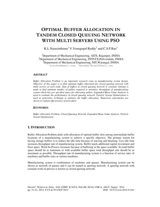
Experiment 2: Total number of pallets=8, Mu= [1, 2], Servers [1, 2]

6. 38 Computer Science Information Technology (CS IT)
Table 4. Complete Enumeration for total number of pallets=8, Mu= [1, 2], Servers [1, 2]
Number
of pallets
Buffer allocation
(1,7) (2,6) (3,5) (4,4) (5,3) (6,2) (7,1)
1 0.6667 0.6667 0.6667 0.6667 0.6667 0.6667 0.6667
2 0.9231 0.9231 0.9231 0.9231 0.9231 0.9231 0.9231
3 0.9376 0.9811 0.9811 0.9811 0.9811 0.9811 0.9699
4 0.9349 0.9841 0.9953 0.9953 0.9953 0.9925 0.976
5 0.9317 0.9822 0.996 0.9988 0.9981 0.9939 0.9766
6 0.9289 0.9791 0.9955 0.9988 0.9985 0.994 0.9766
7 0.9265 0.9757 0.9938 0.9984 0.9983 0.9939 0.9766
8 0.9245 0.9687 0.9915 0.9979 0.9982 0.9939 0.9766
Table 5. Solution using proposed algorithm for total number of pallets=8, Mu= [1 2],
Servers= [1, 2]
Optimum Buffer Allocation Number of Pallets Maximum Throughput
(4,4) 6 0.9988
Experiment 3: Total number of pallets=8, Mu= [2, 1], Servers [1, 3]
Table 6. Complete Enumeration for total number of pallets=8, Mu= [2, 1], Servers [1, 3]
Number
of
pallets
Buffer allocation
(1,7) (2,6) (3,5) (4,4) (5,3) (6,2) (7,1)
1 0.6667 0.6667 0.6667 0.6667 0.6667 0.6667 0.6667
2 1.2 1.2 1.2 1.2 1.2 1.2 1.2
3 1.4851 1.5789 1.5789 1.5789 1.5789 1.5789 1.5152
4 1.5548 1.7042 1.7538 1.7538 1.7538 1.7204 1.5624
5 1.5663 1.7267 1.8197 1.8483 1.8291 1.7395 1.5373
6 1.5667 1.7087 1.8279 1.8749 1.8383 1.7095 1.5207
7 1.5657 1.6826 1.7961 1.8498 1.8044 1.6812 1.5156
8 1.5651 1.6486 1.7362 1.7971 1.7613 1.6611 1.5149
Table 7. Solution using proposed algorithm for total number of pallets=8, Mu= [2 1],
Servers= [1, 3]
Optimum Buffer
Allocation
Number of Pallets Maximum Throughput
(4,4) 6 1.8749
Experiment 4: total number of pallets=16, Mu= [0.2, 0.5], Servers [5, 3]

7. Computer Science Information Technology (CS IT) 39
Table 8. Complete Enumeration for total number of pallets=16, Mu= [0.2, 0.5], Servers [5, 3]
Number
of
pallets
Buffer allocation
(1,15) (2,14) (3,13) (4,12) (5,11) (6,10) (7,9) (8,8)
1 0.1429 0.1429 0.1429 0.1429 0.1429 0.1429 0.1429 0.1429
2 0.2857 0.2857 0.2857 0.2857 0.2857 0.2857 0.2857 0.2857
3 0.4162 0.4286 0.4286 0.4286 0.4286 0.4286 0.4286 0.4286
4 0.5216 0.5667 0.5702 0.5702 0.5702 0.5702 0.5702 0.5702
5 0.594 0.6912 0.7074 0.7086 0.7086 0.7086 0.7086 0.7086
6 0.6256 0.7694 0.8135 0.82 0.8205 0.8205 0.8205 0.8205
7 0.636 0.7887 0.8703 0.8898 0.8928 0.8931 0.8931 0.8931
8 0.6449 0.7713 0.8819 0.9222 0.9317 0.9333 0.9335 0.9335
9 0.6515 0.7484 0.8667 0.9308 0.9512 0.9565 0.9574 0.9575
10 0.6547 0.7293 0.8392 0.9224 0.9571 0.9687 0.9718 0.9724
11 0.656 0.7173 0.8086 0.9025 0.9522 0.9726 0.9795 0.9812
12 0.6566 0.7114 0.7821 0.8749 0.9389 0.9695 0.9818 0.9854
13 0.6568 0.7095 0.7636 0.844 0.9177 0.9599 0.9788 0.9852
14 0.6568 0.7096 0.754 0.8148 0.8887 0.9423 0.9702 0.9808
15 0.6568 0.7104 0.7516 0.7912 0.8531 0.9152 0.9551 0.9726
16 0.6568 0.7111 0.7532 0.7752 0.8158 0.8792 0.9327 0.9608
Number
of
pallets
Buffer allocation
(9,7) (10,6) (11,5) (12,4) (13,3) (14,2) (15,1) (9,7)
1 0.1429 0.1429 0.1429 0.1429 0.1429 0.1429 0.1429 0.1429
2 0.2857 0.2857 0.2857 0.2857 0.2857 0.2857 0.2857 0.2857
3 0.4286 0.4286 0.4286 0.4286 0.4286 0.4286 0.4235 0.4286
4 0.5702 0.5702 0.5702 0.5702 0.5702 0.5683 0.5494 0.5702
5 0.7086 0.7086 0.7086 0.7086 0.7078 0.6996 0.6582 0.7086
6 0.8205 0.8205 0.8205 0.8201 0.8162 0.7952 0.7281 0.8205
7 0.8931 0.8931 0.8929 0.8909 0.8799 0.8416 0.7559 0.8931
8 0.9335 0.9334 0.9322 0.9261 0.9042 0.8504 0.76 0.9335
9 0.9575 0.9568 0.9531 0.94 0.9066 0.8449 0.7589 0.9575
10 0.972 0.9697 0.9616 0.9404 0.8989 0.8379 0.758 0.972
11 0.9802 0.975 0.9615 0.9339 0.89 0.8338 0.7577 0.9802
12 0.9833 0.9748 0.9566 0.926 0.8838 0.8325 0.7576 0.9833
13 0.9824 0.9712 0.9505 0.9196 0.8809 0.8326 0.7576 0.9824
14 0.9786 0.9663 0.945 0.9157 0.8803 0.833 0.7577 0.9786
15 0.9728 0.9613 0.9409 0.914 0.8808 0.8333 0.7577 0.9728
16 0.9659 0.9566 0.9381 0.9136 0.8816 0.8334 0.7577 0.9659
Table 9. Solution using proposed algorithm for total number of pallets=16, Mu= [0.2, 0.5], Servers [5, 3]
Optimum Buffer
Allocation
Number of Pallets Maximum Throughput
(8,8) 12 0.9854
Experiment 5: Total number of pallets=7, Mu= [2, 0.1, 1], Servers [1, 2, 1]

8. 40 Computer Science Information Technology (CS IT)
Table 10. Complete Enumeration for total number of pallets=7, Mu= [2, 0.1, 1], Servers [1, 2, 1]
Number
of
pallets
Buffer allocation
(1,1,5) (1,2,4) (1,3,3) (1,4,2) (1,5,1) (2,1,4) (2,2,3) (2,3,2)
1 0.087 0.087 0.087 0.087 0.087 0.087 0.087 0.087
2 0.1723 0.1723 0.1723 0.1723 0.1723 0.1723 0.1723 0.1723
3 0.1933 0.1938 0.1938 0.1938 0.1934 0.1933 0.1938 0.1938
4 0.1974 0.1986 0.1987 0.1986 0.1976 0.1974 0.1986 0.1986
5 0.1982 0.1996 0.1997 0.1995 0.1983 0.1982 0.1996 0.1995
6 0.1982 0.1998 0.1999 0.1997 0.1984 0.1982 0.1998 0.1996
7 0.1981 0.1998 0.1999 0.1997 0.1984 0.1981 0.1998 0.1997
Number
of pallets
Buffer allocation
(2,4,1) (3,1,3) (3,2,2) (3,3,1) (4,1,2) (4,2,1) (5,1,1)
1 0.087 0.087 0.087 0.087 0.087 0.087 0.087
2 0.1723 0.1723 0.1723 0.1723 0.1723 0.1723 0.1723
3 0.1934 0.1933 0.1938 0.1934 0.1933 0.1934 0.1929
4 0.1976 0.1974 0.1986 0.1976 0.1974 0.1976 0.1964
5 0.1983 0.1982 0.1994 0.1983 0.198 0.1982 0.1968
6 0.1984 0.1982 0.1995 0.1984 0.198 0.1983 0.1968
7 0.1984 0.1981 0.1995 0.1984 0.1979 0.1983 0.1967
Table 11. Solution using proposed algorithm for total number of pallets=7, Mu= [2, 0.1, 1],
Servers [1, 2, 1]
Optimum Buffer
Allocation
Number of Pallets Maximum Throughput
(1, 3, 3) 7 0.1999
Experiment 6: Experiments were conducted for 3 node closed queuing network with various total
buffer sizes. Results are shown in table 12.
Table 12. Optimum solutions for 3 node network
Total
buffer
space
Service rates Number
of
servers
Optimum
Buffer
Allocation
Optimum
number
of pallets
Maximum
Throughput
12 (0.3333,1,1) (3,1,1) (4,4,4) 10 0.7743
15 (0.3333,0.5,0.3333) (3,2,3) (5,5,5) 13 0.8047
15 (1,1.5,3) (2,2,1) (6,6,3) 11 1.9269
Experiment 7: Experiments were conducted for 5 node closed queuing network with various total
buffer sizes. Results are shown in table 13.

9. Computer Science Information Technology (CS IT) 41
Table 13. Optimum solutions for 5 node network
Total
buffer
space
Service rates Number
of servers
Optimum
Buffer
Allocation
Optimum
number of
pallets
Maximum
Throughput
25 (0.8,0.8,0.8,0.8,0.8) (3,2,1,2,3) (1,1,10,11,2) 20 0.7998
33 (4,1,3,2,1.5) (1,5,2,2,3) (8,9,3,4,9) 31 3.6758
Experiment 8: Experiments were conducted for 8 node closed queuing network with various total
buffer sizes. Results are shown in table 14.
Table 14. Optimum solutions for 8 node network
Present work is focused on multi server reliable machines. Work can be extended to solve merge,
split, unreliable systems. Extension of this work is under progress by the authors.
REFERENCES
[1] Daskalaki, S., Smith, J. M. (2004). Combining routing and buffer allocation problems in serial-parallel
queuing networks. Annals of Operations Research, 125, 47–68.
[2] Smith, J. M., Cruz, F. R. B. (2005). The buffer allocation problem for general finite buffer queuing
networks. IIE Transactions,37(4), 343–365.
[3] Smith, J. M., Cruz, F. R. B., Van Woensel, T. (2010). Topological networks design of general,
finite, multi-server queueing networks. European Journal of Operational Research, 201(2), 427–441.
[4] Cruz, F. R. B., Duarte, A. R., Van Woensel, T. (2008). Buffer Allocation in general single-server
queuing networks. Computers, Operations Research 35(11), 3581-3598.
[5] Yuzukirmizi, M., Smith, J. M. (2008). Optimal buffer allocation in finite closed networks with
multiple servers. Computers, Operations Research, 35, 2579-2598.
[6] Cruz, F. R. B., Van Woensel, T., Smith, J. M. (2010). Buffer and throughput trade-offs in M/G/1/K
queuing networks: A bicriteria approach. International Journal of Production Economics, 125, 224–
234.
[7] Cruz, F. R. B., Kendall, G., While, L., Duarte, A. R., Brito, N.L.C.(2012). Throughput maximization
of queueing networks with simultaneous minimization of service rates and buffers. Mathematical
Problems in Engineering. Volume 2012, Article ID 692593.
[8] Seo, D-W., Lee, H. (2011). Stationary waiting times in m-node tandem queues with production
blocking. IEEE Transactions on Automatic Control, 56(4), 958-961.