Similarity and Variance of Color Difference Based Demosaicing

TELKOMNIKA Indonesian Journal of Electrical Engineering
Vol. 13, No. 2, February 2015, pp. 238 ~ 246
DOI: 10.11591/telkomnika.v13i2.7048  238
Received August 2, 2014; Revised September 18, 2014; Accepted October 16, 2014
Similarity and Variance of Color Difference Based
Demosaicing
R.Niruban*1
, T.Sree Renga Raja2
, R.Deepa3
1
Sathyabama University, Chennai
2
Electrical and Electronics Engineering, Anna University (BIT Campus), Tiruchirapalli, India
3
Computer Science and Engineering, Prince Dr.K.Vasudevan College of Engineering and Technology,
Chennai, India.
*Corresponding author, e-mail: nirubanme@gmail.com
1
, renga_raja@rediffmail.com
2
,
rkdeepa14@gmail.com
3
Abstract
The aim of the project is to find the missing color samples at each pixel location by the
combination of similarity algorithm and the variance of colour difference algorithm. Many demosaicing
algorithms find edges in horizontal and vertical directions, which are not suitable for other directions.
Hence using the similarity algorithm the edges are found in different directions. But in this similarity
algorithm sometimes the horizontal and vertical directions are mislead. Hence this problem can be rectified
using the variance of colour difference algorithm. It is proved experimentally that this new demosaicing
algorithm based on similarity and variance of colouyr difference has better colour peak signal to noise ratio
(CPSNR). It has better o0bjective and subjective performance. It is an analysis study of both similarity and
colour variance algorithms.
Keywords: colour filter array, demosaicing, unified high frequency map, peak signal to noise ratio,
acquisition
Copyright © 2014 Institute of Advanced Engineering and Science. All rights reserved.
1. INTRODUCTION
Digital cameras become and many people are choosing to take pictures with digital
cameras instead of film cameras. When a digital image is recorded, the camera needs to
perform a significant amount of processing to provide the user a viewable image. This
processing includes white balance adjustments, gamma correction, compression and more.
Most consumer digital cameras capture colour information with a single light sensor and a
colour filter array (CFA). The CFA is compound by a set of spectrally selective filters, arranged
in an interleaved mosaic pattern, so that in each pixel samples only one of the components of
the colour spectrum is captured instead of capturing three color samples(typically red,green,and
blue) at each pixel location ,these camera capture a so called ‘mosaic’ image, where only one
color is sampled at each location. The two missing colors must be interpolated from the
surrounding sample. A very important part of this image processing is called color filter array
interpolation or demosaicing.
A color image requires atleast three color samples at each pixel location. Computer
images often use red, blue and green. A camera would need three separate sensors to
completely measure the image. Using multiple sensors to detect different parts of the visible
spectrum requires splitting the light entering the camera, so that the scene is image onto each
sensor. Precise registration is then required to align the three images. These additional
requirements add a large expense to the system. Thus, many cameras use a single sensor with
a color filter array. The color filter array allows only one part of the spectrum to pass to the
sensor so that only one color is measured at each pixel. This means that the camera must
eliminate the missing two color values at each pixel. This process is known as demosaicing.
The choice of the best color filter array is very important for the final image quality and different
solution. The best color filter array is the bayer pattern which is proved as the standard pattern.
The sample bayer pattern is shown below in Figure 1.

TELKOMNIKA ISSN: 2302-4046 
Similarity and Variance of Color Difference Based Demosaicing (R.Niruban)
239
G00 R01 G02 R03 G04 R05
B10 G11 B12 G03 B14 G15
G20 R21 G22 R23 G24 R25
B30 G31 B32 G33 B34 G35
G40 R41 G42 R43 G44 R45
B50 G51 B52 G53 B54 G55
Figure 1. Bayer pattern
Digital still color cameras are based on a single charge coupled device(CCD) array or
complementary metal oxide semiconductor (CMOS) sensors and capture color information by
using three or more color filters, each sample point capturing only one sample of the color
spectrum. In a three-chip color camera, the light entering the camera is split and projected on to
each spectral sensor. Each sensor requires its proper driving electrons, and the sensors have to
be registered precisely. These additional requirements had a large expense to the system. To
reduce cost and complexity, digital camera manufacturers use a single CCD/CMOS sensor with
a color filter array (CFA) to capture all the three primary colors (R,G,B) at the same time.
Color filter arrays containing one or more colors for liquid crystal displays and other
opto-electronic devices are made by using a laser to ablate portions of a coating on either a
colored or transparent substrate. Color filter material are placed into the ablated openings and
cured. The number of laser–ablated openings in the coated substrate varies, depending on the
quality and type of color desired.
2. Review of Similarity Based Demosaicing Algorithm
Similarity based demosaicing algorithms has two forms. one is the without refinement
form and the other is the with refinement form. In this UHF map acquisition and similarity based
interpolation comes under without refinement and global edge classification of horizontal and
vertical direction comes under with refinement method. In the without refinement method we
calculate the map index using the high frequency components and using this map values we
are interpolating the missing pixels in horizontal and vertical direction using global edge
classifier separately in the refining method. This further gives better color peak signal to noise
ratio (CPSNR) value. This is the similarity based demosaicing algorithm.
In this algorithm the unified high frequency map is formed by taking the average of
every sample of red, blue and green components independently and then every sample values
are independently subtracted from the average value. Then we have to note that these values
are larger than zero or lesser than zero. If the values larger than zero then we have to plot that
particular value as one and if the differenced value is lesser than zero then we have to plot the
value as zero. Like this the unified high frequency map is formed. Based on this the direction of
the edge is found out and the missing samples are interpolated.
ʎ(i,j)=
0, , 0
1,
(1)
Where ʎ(i,j) is the map index to be calculated and h(i,j) is the difference between the individual
pixels and the average of the total pixels. The map index calculations are shown below in
Figure 2.

 ISSN: 2302-4046
TELKOMNIKA Vol. 13, No. 2, February 2015 : 238 – 246
240
153 134 208
145 151 178
40 83 147
145 161 197
147 165 203
75 98 159
69 101 160
23 68 95
19 62 93
63 139 155
28 65 99
18 33 69
(a) Map Index calculations
1 1 1 1 1 1
0 1 1 1 1 1
0 1 0 1 1 1
0 0 0 0 1 1
0 0 0 0 0 1
0 0 0 0 0 0
(b) Unified High Frequency Map
Figure 2. Flow chart of map index calculations

241
In the above figure the map value for each pixel is found out by taking the difference
between the individual pixels and the average of the total pixels are shown. While plotting the
map in the differenced value is greater than zero then the particular map value is plotted as 1
and if the differenced value is less than zero then that particular value is plotted as 0.
Now after forming the map the missing pixels are interpolated using the map direction.
Initially the green samples are interpolated by using the comparison of the map values of the
neighboring green samples. If they are same then the formula to find the missing green samples
are given below.
∑ /2 .
1,
0,
(2)
The diagram for interpolating the missing green samples are shown below in Figure 3
in which 1 and values are the same then the green values are interpolated by using the
formula (2).
A0
G0
A1 G1 AC G2 A2
G3
A3
(a) CFA Data
λ0
λ 1 λ C λ 2
λ 3
(b) UHF Map
Figure 3. Interpolation of missing green sample

 ISSN: 2302-4046
242
If the map values are not the same then we have to interpolate the missing green
samples as below.
ρ= Gl (3)
After interpolating the missing green samples, the missing red and blue samples are
interpolated by comparing the map values. The missing red and blue samples are interpolated
as by interpolating the missing red and blue samples in the green samples which are already
present. Then the missing red samples are interpolated in the blue samples present and then
the missing blue samples are interpolated in the red samples which are already present. The
missing red and blue samples are interpolated as by the formula given below.
Now the missing red samples in the blue samples present and the missing
blue samples in the red samples present are interpolated using the formula given below.
, , ∑ , . , , , .,
1, , ,
0,
(4)
Here also if the map values are not the same then we have to interpolate the missing samples
as below:
∑ , ,, (5)
Now the missing red and blue samples in the green samples, which are already present
are obtained using the formula given below.
a(s,t)=G(s,t)+{(A(s,t-1)-G(s,t-1))+(A(s,t+1)-G(s,t+1))}/2 (6)
a(s,t)=G(s,t)+{(A(s-1,t)-G(s-1,t))+(A(s+1,t)-G(s+1,t))}/2 (7)
3. Review of Variance of Color Difference Algorithm
In this variance of color difference algorithm the missing green samples are interpolated
in raster scan manner as shown below. Initially the green sample is interpolated in a raster scan
manner and then the missing red and blue components are interpolated based on the green
samples which we already interpolated. Figure 4 shown below is the bayer pattern with red as
centre,blue as centre and green as centre respectively using which the missing green samples
are interpolated in a raster scan manner.
Figure 4. Interpolation of missing green samples in raster scan manner
To find the missing green samples in a raster scan manner it is necessary to find the
edge direction which may be horizontal or vertical. If the edge direction is horizontal then the
green samples are interpolated according to the formula (8) below.

243
,
, , , , ,

(8)
In this equation small g represents the green samples to be interpolated and the G
represents the green samples which are already present. If the edge direction is vertical then
the formula to find the missing green sample is shown Equation (9).
,
, , , , , , ,

(9)
After interpolating the missing green samples according to the edge direction, the
missing red and blue samples are interpolated. The formula to find the missing red and blue
samples is given below in the Equation (10) and (11) respectively.
, ,
, , , ,
(10)
, ,
, , , ,
(11)
In the above equation r and b represents the missing red and blue samples to be
interpolated. G,R,B represents the green, blue, and red samples which are already present.
4. Proposed Algorithm
In the similarity based demosaicing algorithm the missing color samples are
interpolated in horizontal,vertical and in diagonal direction. But it sometimes mislead the
horizontal and vertical directions. In variance of color difference algorithm only the horizontal
and vertical directions are detected. So in this algorithm it is the analysis of the both similarity
based demosaicing algorithm and variance of color difference algorithm in which by combining
both the algorithm a new algorithm called demosaicing based on similarity and variance of color
difference is found out.
In this new algorithm initially the unified high frequency map is formed and based on
that the edge directions are detected. After detecting the edge direction the missing green
samples are interpolated based on the similarity algorithm and the missing red and blue
samples are interpolated according to the same similarity algorithm. Now using the variance of
color difference algorithm again the missing green samples are interpolated in a raster scan
manner, trhen the missing red and blue samples are interpolated according to the interpolated
green samples using the variance of color difference algorithm.
The new method by combining the similarity based demosaicing algorithm and the variance of
color difference algorithm given below in Equation (12), (13).
Similarity image=merged image (12)
Merged image=reconstructed color variance image (13)
In this new algorithm by combining the similarity based demosaicing algorithm and the
variance of color difference algorithm the edge directions are detected perfectly without any
misleading in any edge directions. Using this analysis of both similarity and color variance
algorithm the edge directions are detected in horizontal, vertical and diagonal directions.
5. Experimental Results
The experimental results of the demosaicing based on similarity and variance of color
difference are shown below. The peak signal to noise ratio of this new algorithm is shown
below. The formula used to find the peak signal to noise ratio is shown below in Equation (14).
10 log
∑ ∑ , ,
(14)

 ISSN: 2302-4046
244
Where o(s,t)=[o(s,t)0,o(s,t)1,o(s,t)2] and the x(s,t)=[x(s,t)0,x(s,t)1,x(s,t)2] denoted the co-
ordinates (s,t) of original and restored image respectively. The comparison tabulation of the
similarity algorithm, variance of color difference algorithm and the proposed algorithm are
shown.
The test images used for the analysis are shown above in the Figure 5. In this the 24
images are tested for the three algorithms and experimentally it is proved that the proposed
algorithm has the better result when compared to the similarity and color variance algorithm.
Figure 5. Kodak test images used for experiment
In the tabular column below it is proved that the proposed algorithm has the better result
for the red, green, blue samples. The best values are marked in bold.
Table 1. Comparison of similarity algorithm, color variance algorithm and proposed algorithm
Image
number
Similarity based demosaicing
algorithm
Variance of color difference
algorithm
Proposed method
R G B R G B R G B
1 34.02 34.48 34.04 25.23 33.48 26.36 34.02 34.48 34.04
2 36.43 39.52 37.98 15.02 39.82 25.36 40.44 43.41 43.81
3 39.78 41.27 39.67 23.28 41.13 20.48 44.12 45.07 43.38
4 36.75 40.38 40.08 18.49 40.36 30.39 40.13 43.52 44.84
5 34.48 34.11 34.33 25.65 34.58 25.33 39.46 38.16 38.98
6 35.31 35.86 35.29 28.61 34.42 23.23 40.49 39.33 39.40
7 39.62 40.25 39.02 26.40 40.75 24.35 43.96 43.88 42.53
8 31.03 32.17 31.17 26.56 31.01 26.83 37.10 36.01 37.73
9 38.09 40.30 39.75 30.70 40.18 27.07 43.88 44.28 44.22
10 39.07 40.25 39.63 29.98 39.93 31.06 43.77 44.00 43.74
11 36.14 36.89 36.74 25.46 36.19 28.90 40.10 40.37 41.08
12 39.75 40.96 39.94 27.12 40.50 23.92 44.23 44.69 43.71
13 31.93 31.48 31.47 28.75 30.17 23.08 37.14 34.32 35.11
14 34.17 36.20 34.23 24.30 36.35 21.07 38.81 39.87 39.49
15 36.48 39.25 38.76 20.16 38.23 27.85 39.84 42.66 43.84
16 38.56 39.32 38.48 33.18 38.04 28.46 44.67 42.94 42.50
17 38.86 39.27 38.71 32.36 38.54 30.96 43.39 42.30 42.62
18 34.37 35.56 35.34 25.89 33.00 23.52 38.87 38.20 39.21
19 35.36 36.58 36.23 28.63 34.89 25.28 39.70 40.47 40.44
20 38.67 39.13 37.84 32.64 37.58 24.41 43.68 42.20 41.72
21 36.02 36.32 35.63 26.59 34.71 27.00 40.68 39.43 39.68
22 35.81 37.33 35.84 26.01 36.27 23.43 39.64 40.48 40.44
23 39.74 41.52 40.32 20.16 39.17 19.17 44.23 45.36 45.44
24 33.39 33.99 32.32 29.01 32.42 26.00 38.81 36.85 36.58

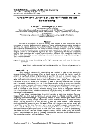
245
Figure 7. PSNR comparison of blue samples for similarity, color variance and proposed
algorithms
Figure 8. PSNR comparison of red samples for similarity, color variance and proposed
algorithms
Figure 9. PSNR comparison of green samples for similarity, color variance and proposed
algorithms
15
20
25
30
35
40
45
50
1 2 3 4 5 6 7 8 9 101112131415161718192021222324
PSNR values
images
Blue PSNR
bpsnr
cvbpsnr
mebpsnr
0
5
10
15
20
25
30
35
40
45
50
1 3 5 7 9 11 13 15 17 19 21 23
PSNR values
images
Red PSNR
rpsnr
cvrpsnr
merpsnr
0
5
10
15
20
25
30
35
40
45
50
1 2 3 4 5 6 7 8 9 101112131415161718192021222324
PSNR values
images
Green PSNR
gpsnr
cvgpsnr
megpsnr

 ISSN: 2302-4046
246
The graphs comparing the similarity algorithm, color variance algorithm and the
proposed algorithm are shown in below. Figure 7 shows the comparison of blue sample for
three algorithms. Figure 8 shows the comparison of red sample for three algorithms. Figure 9
shows the comparison of green sample for three algorithms.
6. Conclusion
In this paper, we introduce a new algorithm by combining similarity and color variance
algorithms called similarity and color difference based demosaicing.we confirmed through the
experiments that the proposed algorithm has better quality improvement than the similarity and
color variance algorithms. Exploration of the proposed algorithms with the situation identifying
the parameters in which similarity and color variance algorithms are adaptively implemented in
real life is worth for further investigation.
References
[1] Adele Droblas Greenberg, Seth Greenberg. Digital Images: A practical guide. Tata McGraw Hill
publications limited. 1995.
[2] Bayer BE. Color imaging array. 1976. U.S.Patent 3971 065.
[3] Gunturk BK, Altunbask Y, Mersereau. Color plane interpolation using alternating projections. IEEE
transactions on image processing. 2002; 11(9): 997-1013.
[4] Daniel M, Stefano. A. Demosiacing with directional filtering and posteriori decision. IEEE transaction
on image processing. 2007; 16(1); 132-141.
[5] Hamilton JF, Adams JE. Adaptive color plane interpolation in single sensor electronic camera. U.S.
Patent. 1987; 5: 629 678.
[6] Chung-Yen S, Wen Chung K. Effective demosaicing using subband correlation. IEEE transaction.
2009; 55(1): 199-204.
[7] King-Kong-chung, Yuk-Hee Chan. Color demosaicing using variance of color differences. IEEE
transaction on Image processing.
[8] Kuo Liang Chunk, Wen-Jen Yang Wen-Ming Yan, Chung-ChouWang. Demosaicing of color filter array
captured images using gradient edge detection masks and adaptive heterogeneity projection. IEEE
transaction on image processing. 2008; 17(12): 2356-2367.
[9] Milan Sonka, Vaclav Hlavac, Roger Boyle. Digital image processing and computer vision. Cengage
Learning. 2008.
[10] Rafael C Gonzales, Richard E Woods. Digital image processing. Pearson Education, Inc, Prentice
Hall publication. 2009.
[11] Rafael C Gonzales, Sleven L Eddins, Richard E Woods. Digital image processing using MATLAB.
Pearson Education, Inc, Prentice Hall publication.
[12] Xin Li, Micheal T Orchard. New edge directed Interpolation. IEEE transactionon image processing.
2001; 10(10): 1521-1527.
[13] Xin L. Demosaicing by successive approximation. IEEE transaction on image processing. 2005; 2005;
14(3): 370-379.
[14] Yuji Itoh. Similarity based demosaicing using unified high frequency map. IEEE transaction on image
processing. 2012; 57(2): 597-605.

Similarity and Variance of Color Difference Based Demosaicing

Recommended

Recommended

More Related Content

What's hot

What's hot (20)

Similar to Similarity and Variance of Color Difference Based Demosaicing

Similar to Similarity and Variance of Color Difference Based Demosaicing (20)

More from Radita Apriana

More from Radita Apriana (20)

Recently uploaded

Recently uploaded (20)

Similarity and Variance of Color Difference Based Demosaicing