1. DERIVATIVES IN MULTI
PORAMATE (TOM) PRANAYANUNTANA
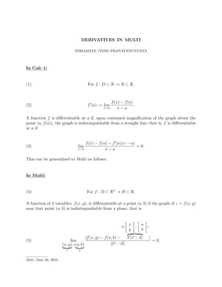
In Calc 1:
For f : D ⊂ R → R ⊂ R,(1)
f (a) := lim
x→a
f(x) − f(a)
x − a
.(2)
A function f is differentiable at a if, upon continued magnification of the graph about the
point (a, f(a)), the graph is indistinguishable from a straight line; that is, f is differentiable
at a if
lim
x→a
f(x) − f(a) − f (a)(x − a)
x − a
= 0.(3)
This can be generalized to Multi as follows:
In Multi:
For f : D ⊂ R2
→ R ⊂ R,(4)
A function of 2 variables, f(x, y), is differentiable at a point (a, b) if the graph of z = f(x, y)
near that point (a, b) is indistinguishable from a plane; that is
lim
(x, y)
r
→(a, b)
a
|f(x, y) − f(a, b) −
T(


x
y

−


a
b

)
T(r − a) |
r − a
= 0,(5)
Date: June 20, 2015.

2. Derivatives in Multi Poramate (Tom) Pranayanuntana
or, from an equation of the tangent plane z = L(x, y) = f(a, b)+fx(a, b)(x−a)+fy(a, b)(y−b)
(if it uniquely exists), we have f(x, y) is differentiable at a point (a, b) if
lim
(x, y)
r
→(a, b)
a
|f(x, y) −
L(x,y)
(f(a, b) + fx(a, b)(x − a) + fy(a, b)(y − b)) |
x
y
−
a
b
= 0.(6)
L(x, y) = f(a, b) + fx(a, b) fy(a, b)
Jf(a)=Jf(a,b)
x − a
y − b
T(r−a)
(7)
= f(a, b) +





fx(a, b)
fy(a, b)
grad f(a,b)= f(a,b)
x − a
y − b





,
where (◦) =
∂(◦)/∂x
∂(◦)/∂y
=
(◦)x
(◦)y
is a vector derivative operator.
Compare the following:
Calc 1 Multi
lim
x→a
|f(x) −
l(x): tangent line of f at a
(f(a) + f (a)(x − a)) |
|x − a|
= 0 lim
r→a
|f(r) −
L(r): tangent plane of f at a
(f(a) + Jf(a)(r − a)) |
r − a
= 0
We can see that Jf(a) is the derivative of z = f(r) = f(x, y) at r = a = (a, b).
In this class, we will use dot product instead of matrix multiplication, so the derivative
matrix Jf(a) will be represented by the gradient vector, grad f(a, b) =
fx(a, b)
fy(a, b)
, in the
xy-plane, which the domain of f is part of.
June 20, 2015 Page 2 of 5

3. Derivatives in Multi Poramate (Tom) Pranayanuntana
Directional Derivatives
Calc 1
∆y = f(x) − f(a) ≈ f (a)(x − a) = f (a)∆x
(8)
= (f (a) · ˆu) |∆x|
= Dˆuf(a) |∆x| ,
where ˆu is the unit vector pointing in the di-
rection of ∆x = x − a.
Multi
∆z = f(r) − f(a) ≈ Jf(a)(r − a)(9)
= (grad f(a, b) (r − a))
= (grad f(a, b) ˆu) r − a
= Dˆuf(a, b) r − a ,
where ˆu is the unit vector pointing in the
direction of ∆r = r − a.
The directional derivative of f(x, y) at (a, b) in the direction of ˆu =
∆r
∆r
in the domain of f
in the xy-plane, denoted by Dˆuf(a, b), is lim
Run→0
Rise
Run
= lim
∆r →0
∆z
∆r
= f(a, b)
∆r
∆r
=
( f(a, b) ˆu).
June 20, 2015 Page 3 of 5

4. Derivatives in Multi Poramate (Tom) Pranayanuntana
It can also be seen that
Dˆuf(a, b) := lim
Run=h→0
Rise
f(a+hu1,b+hu2)
f(
a
b
+ h
u1
u2
) −f(a, b)
h
Run
(10)
= lim
h=0,h→0
f(
x
a + hu1,
y
b + hu2) − f(a, b)
h
;
with f(x, y) − f(a, b) ≈ fx(a, b)(x − a) + fy(a, b)(y − b)
= lim
h=0,h→0
fx(a, b)(hu1) + fy(a, b)(hu2)
h
=
fx(a, b)
fy(a, b)
u1
u2
= ( f(a, b) ˆu)
= f(a, b) ˆu cos θ, 0 ≤ θ ≤ π.
June 20, 2015 Page 4 of 5

5. Derivatives in Multi Poramate (Tom) Pranayanuntana
From Dˆuf(a, b) = f(a, b) ˆu cos θ, 0 ≤ θ ≤ π. Since ˆu = 1 and f(a, b) is a fixed
positive number (once point (a, b) is picked), therefore
max Dˆuf(a, b) = f(a, b) , when cos θ = 1 that is when θ = 0 or when ˆu points in direction
of f(a, b).
∆z = f(r) − f(a) ≈ Jf(a)(r − a)
= (grad f(a, b) (r − a))
= (grad f(a, b) ˆu) r − a
= Dˆuf(a, b) r − a .
Properties of grad f(a, b) = f(a, b)
If f(a, b) = 0. Then
Direction Properties



• f(a, b) points in direction of maximum rate of increasing of f(a, b),
• Direction of f(a, b) is perpendicular to the contour line z = f(a, b)
(in the domain of f in the xy-plane)
Magnitude Properties



• max Dˆu= f(a,b)/ f(a,b) f(a, b) = f(a, b)
1
ˆu :1
cos 0
That is f(a, b) = max Dˆuf(a, b) or
f(a, b) = maximum rate of change of f at (a, b)
• f(a, b)
is large when contour lines (of fixed ∆z) of f are closer together.
is small when contour lines (of fixed ∆z) of f are further apart.
June 20, 2015 Page 5 of 5