OBSERVATIONAL STUDY
Dr. Partha Sarkar
(PGT, 2nd Yr)
Department of Pharmacology
Medical College, Kolkata
STUDY DESIGN
Observational
Analytical
 Cross sectional
 Cohort
 Case control
Descriptive
 Case report
 Case series
 surveys
Experimental
 RCT
 QUASI
Study Design
Observational vs. Experimental Study
Observational studies
The population is observed without any interference by
the investigator
Experimental studies
The investigator tries to control the environment in which
the hypothesis is tested (the randomized, double-blind
clinical trial is the gold standard)
Observational Study
• Non-experimental
• Observational because there is no individual
intervention
• Treatment and exposures occur in a “non-
controlled” environment
• Individuals can be observed prospectively,
retrospectively, or currently
Limitation of observational research:
confounding
Confounding:
Risk factors don’t happen in isolation, except in
a controlled experiment.
Example
Breastfeeding has been linked to higher IQ in infants,
but the association could be due to confounding by
socioeconomic status. Women who breastfeed tend to
be better educated and have better prenatal care,
which may explain the higher IQ in their infants.
Cause and Effect?
Atherosclerosis
Depression in
elderly
?
Biological changes
?
Lack of exercise
Poor Eating
Advancing
Age
Why Observational Studies?
 Cheaper
 Faster
 Can examine long-term effects
 Hypothesis-generating
 Sometimes, experimental studies are not ethical
(e.g- Randomizing subjects to smoke)
Descriptive Studies
Good descriptive reporting answers five basic W questions:
Who, what, why, when, where
 Case report
 Case-series reports
 Surveillance studies
And a sixth: so what ?
Who has the disease in question ?
What is the condition or disease being studied ?
Why did the condition or disease arise ?
Where does or does not the condition arise?
Descriptive studies
Case Report
Case Series
Descriptive
Epidemiology Study
One case of unusual findings
Multiple cases of
findings
Population-based
cases with denominator
Descriptive studies
Case Reports
 Detailed presentation of a single case or handful of cases
 Generally report a new or unique finding
e.g- • previous undescribed diseas
• unexpected link between diseas
• unexpected new therapeutic effect
• adverse events
Case Series
 Experience of a group of patients with a similar diagnosis
 Assesses prevalent disease
 Cases may be identified from a single or multiple sources
 Generally report on new/unique condition
 May be only realistic design for rare disorders
 Advantages
• Useful for hypothesis generation
• Informative for very rare disease with few
established risk factors
• Characterizes averages for disorder
 Disadvantages
• Cannot study cause and effect relationships
• Cannot assess disease frequency
Case Series
Analytical Studies
Look to link exposure and disease
 What is the exposure?
 Who are the exposed?
 What are the potential health effects?
 What approach will you take to study the relationship
between exposure and effect?
Basic Question in Analytic Epidemiology
 Are exposure and disease linked?
Exposure Disease
Analytical Stdies
Analytical Stdies
Cross-sectional studies
 An “observational” design that surveys exposures
and disease status at a single point in time (a cross-
section of the population)
time
Study only exists at this point in time
Cross-sectional Design
time
Study only exists at this point in time
Study
population
No Disease
Disease
factor present
factor absent
factor present
factor absent
Cross-sectional Studies
 Often used to study conditions that are relatively frequent
with long duration of expression
(nonfatal, chronic conditions)
 It measures prevalence, not incidence of disease
 Example: community surveys
 Not suitable for studying rare or highly fatal diseases
or a disease with short duration of expression
Cross-sectional studies
Disadvantages
 Weakest observational design,(it measures prevalence,
not incidence of disease). Prevalent cases are survivors
 The temporal sequence of exposure and effect may be
difficult or impossible to determine
 Usually don’t know when disease occurred
 Rare events a problem. Quickly emerging diseases a
problem
Cross-sectional study
 Relationship between atherosclerosis and late-life
depression (Tiemeier et al. Arch Gen Psychiatry, 2004).
Methods
Researchers measured the prevalence of coronary
artery calcification (atherosclerosis) and the prevalence
of depressive symptoms in a large cohort of elderly men
and women in Rotterdam (n=1920).
Coronary calc >500 539
Coronary calc <=500 1381
81 1839 1920
Any
depression
None
28 511
53 1328
2.19)(0.86,CI95%;37.1
038.
052.
RR
Risk Ratio
Interpretation: those with coronary calcification are 37%
more likely to have depression (not significant).
Key difference
WHO IS BEING COMPARED?
COHORT: EXPOSED VS. UNEXPOSED
CASE-CONTROL: DISEASED VS. NON-DISEASED
Cohort studies
Sample on exposure status and track disease development
(for rare exposures)
 Marginal probabilities (and rates) of developing
disease for exposure groups are valid.
Timeframe of Studies
Prospective Study
Looks forward, looks to the future, examines future
events, follows a condition, concern or disease into the
future
time
Study begins here
Cohort Studies
Target
population
Exposed
Not Exposed
Disease-free
cohort
Disease
Disease-free
Disease
Disease-free
TIME
Types of cohort study
The Framingham Heart Study
 The Framingham Heart Study was established in
1948, when 5209 residents of Framingham, Mass,
aged 28 to 62 years, were enrolled in a prospective
epidemiologic cohort study.
 Health and lifestyle factors were measured (blood
pressure, weight, exercise, etc.).
 Interim cardiovascular events were ascertained from
medical histories, physical examinations, ECGs, and
review of interim medical record.
Measuring Risk
Cohort Study
What is the probability of getting diseased if you are
exposed as compared to unexposed?
Case-Control Study
What is the probability of having been exposed if
you have the disease compared to not having the
disease?
Risk in Cohort Studies
 Relative Risk (RR)
RR
A A B
C C D




probability of disease given exposed
probability of disease given unexposed
/ ( )
/ ( )
Disease Non-Diseased
Exposed A B A+B
Unexposed C D C+D
A+C B+D
400 400
1100 2600
0.2
3000/400
1500/400 RR
Hypothetical Data
Normal BP
CHF
No CHF
1500 3000
High Systolic BP
Cohort Studies-Advantages/Limitations
Advantages
 Allows you to measure true rates and risks of disease for
the exposed and the unexposed groups.
 Temporality is correct (easier to infer cause and effect).
 Can be used to study multiple outcomes.
 Prevents bias in the ascertainment of exposure that may
occur after a person develops a disease.
Disadvantages
 Can be lengthy and costly! 60 years for Framingham.
 Loss to follow-up is a problem (if non-random)
 Selection Bias: Participation may be associated with
exposure status for some exposures
Case-Control Studies
 Sample on disease status and ask retrospectively about
exposures (for rare diseases)
Marginal probabilities of exposure for cases and controls
are valid.
 Doesn’t require knowledge of the absolute risks of disease
 For rare diseases, can approximate relative risk
Timeframe of Studies
• Retrospective Study
“to look back”, looks back in time to study events
that have already occurred
time
Study begins here
Target
population
Exposed in past
Not exposed
Exposed
Not Exposed
Case-Control Studies
Disease
(Cases)
No Disease
(Controls)
Case-control example
 A study of the relation between body mass index and the
incidence of age-related macular degeneration.
 Methods
Researchers compared 50 Iranian patients with confirmed
age-related macular degeneration and 80 control subjects
with respect to BMI, smoking habits, hypertension, and
diabetes. The researchers were specifically interested in the
relationship of BMI to age-related macular degeneration.
Results
Comparison of BMI in case and control groups
Case n = 50(%) Control n = 80 (%) p Value
Lean BMI <20 7 (14) 6 (7.5) NS
Normal 20 BMI <25 16 (32) 20 (25) NS
Overweight 25 BMI <30 21 (42) 36 (45) NS
Obese BMI 30 6 (12) 18 (22.5) NS
NS, not significant.
Overweight Normal
ARMD 27 23
No ARMD 54 26
What is the risk ratio here?
50
80
There is no risk ratio, because we cannot calculate the
risk of disease!!
Corresponding 2x2 Table
Odds vs. Risk
 We cannot calculate a risk ratio from a case-control
study.
 BUT, we can calculate a measure called the odds
ratio…
Odds vs. Risk
If the risk is… Then the odds
are…
½ (50%)
¾ (75%)
1/10 (10%)
1/100 (1%)
An odds is always higher than its corresponding probability,
unless the probability is 100%
1:1
3:1
1:9
1:99
The proportion of cases and controls
are set by the investigator; therefore,
they do not represent the risk
(probability) of developing disease.
bc
ad
d
c
b
a
dcd
dcc
bab
baa
OR
DEP
DEP
DEP
DEP






)/(
)/(
)/(
)/(
)~/(~
)~/(
)/(~
)/(
Exposure (E) No Exposure (~E)
Disease (D) a b
No Disease (~D) c d
a+b=cases
c+d=controls
Odds of exposure
in the cases
Odds of exposure
in the controls
Odds Ratio
d
b
c
a
d
c
b
a
bc
ad
OR 
Exposure (E) No Exposure (~E)
Disease (D) a b
No Disease (~D) c d
Odds of
disease for
the exposed
Odds of exposure for the controls
Odds of exposure for the cases
Odds of disease
for the unexposed
Odds Ratio
57.
54*23
26*27
26
54
23
27
OR
Overweight Normal
ARMD 27 23
No ARMD 54 26
Can be interpreted as: Overweight people have a 43%
decrease in their ODDS of age-related macular
degeneration. (not statistically significant here)
Odds Ratio
RROR 
 If the disease is rare (affecting <10% of the population)
WHY?
If the disease is rare, the probability of it NOT happening
is close to 1, and the odds is close to the risk. Eg:
50.
10:1
20/1
474.
9/1
19/1


RR
OR
Odds Ratio
 Good approximation of the risk ratio if the disease is rare
The Rare Disease Assumption
RROR EDP
EDP
EDP
EDP
EDP
EDP
 )~/(
)/(
)~/(~
)~/(
)/(~
)/(
1
1
When a disease is rare:
P(~D) = 1 - P(D)  1
The odds ratio vs. the risk ratio
1.0 (null)
Odds ratio
Risk ratio Risk ratio
Odds ratio
Odds ratio
Risk ratio Risk ratio
Odds ratio
Rare Outcome
Common Outcome
1.0 (null)
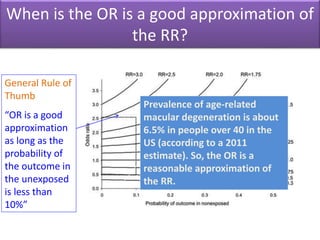
When is the OR is a good approximation of
the RR?
General Rule of
Thumb
“OR is a good
approximation
as long as the
probability of
the outcome in
the unexposed
is less than
10%”
Prevalence of age-related
macular degeneration is about
6.5% in people over 40 in the
US (according to a 2011
estimate). So, the OR is a
reasonable approximation of
the RR.
Case-control studies
Advantages/Limitations:
• Advantages
– Cheap and fast
– Efficient for rare diseases
• Disadvantages
– Getting comparable controls is often tricky
– Temporality is a problem (did risk factor cause disease or
disease cause risk factor?
– Recall bias
Nested case-control studies
 A case-control study nested within a cohort study
 Ideal for predictor variables that are expensive to
measure and that can be assessed at the end of
the study on subjects who develop the outcome
during the study (cases) and on a sample of those
who do not (controls)
 Because the number of cases is probably fairly small, can
match multiple controls to a given case to increase the
power.
Why use a nested case-control study?
 Removes recall bias because data collected before
development of disease.
 Allows for the time element to be included in the case-
control. Therefore, if abnormal biologic characteristics
were found years before the disease developed, these
findings could now be attributed to risk factors for the
disease rather than potential developments of early,
subclinical disease.
 Often more cost-effective than a cohort. Not all samples
collected are tested. Rather they are stored until the
disease has developed at which time analysis begins.
Table Size Test or measures of association
2x2 Risk ratio (cohort or cross-sectional studies)
Odds ratio (case-control studies)
Chi-square
Difference in proportions
Fisher’s Exact test (cell size less than 5)
RxC Chi-square
Fisher’s Exact test (expected cell size >5)
Summary of statistical tests for
contingency tables
THANK YOU

observational analytical study

  • 1.
    OBSERVATIONAL STUDY Dr. ParthaSarkar (PGT, 2nd Yr) Department of Pharmacology Medical College, Kolkata
  • 2.
    STUDY DESIGN Observational Analytical  Crosssectional  Cohort  Case control Descriptive  Case report  Case series  surveys Experimental  RCT  QUASI
  • 3.
  • 4.
    Observational vs. ExperimentalStudy Observational studies The population is observed without any interference by the investigator Experimental studies The investigator tries to control the environment in which the hypothesis is tested (the randomized, double-blind clinical trial is the gold standard)
  • 5.
    Observational Study • Non-experimental •Observational because there is no individual intervention • Treatment and exposures occur in a “non- controlled” environment • Individuals can be observed prospectively, retrospectively, or currently
  • 6.
    Limitation of observationalresearch: confounding Confounding: Risk factors don’t happen in isolation, except in a controlled experiment. Example Breastfeeding has been linked to higher IQ in infants, but the association could be due to confounding by socioeconomic status. Women who breastfeed tend to be better educated and have better prenatal care, which may explain the higher IQ in their infants.
  • 7.
    Cause and Effect? Atherosclerosis Depressionin elderly ? Biological changes ? Lack of exercise Poor Eating Advancing Age
  • 8.
    Why Observational Studies? Cheaper  Faster  Can examine long-term effects  Hypothesis-generating  Sometimes, experimental studies are not ethical (e.g- Randomizing subjects to smoke)
  • 9.
  • 10.
    Good descriptive reportinganswers five basic W questions: Who, what, why, when, where  Case report  Case-series reports  Surveillance studies And a sixth: so what ? Who has the disease in question ? What is the condition or disease being studied ? Why did the condition or disease arise ? Where does or does not the condition arise? Descriptive studies
  • 11.
    Case Report Case Series Descriptive EpidemiologyStudy One case of unusual findings Multiple cases of findings Population-based cases with denominator Descriptive studies
  • 12.
    Case Reports  Detailedpresentation of a single case or handful of cases  Generally report a new or unique finding e.g- • previous undescribed diseas • unexpected link between diseas • unexpected new therapeutic effect • adverse events
  • 13.
    Case Series  Experienceof a group of patients with a similar diagnosis  Assesses prevalent disease  Cases may be identified from a single or multiple sources  Generally report on new/unique condition  May be only realistic design for rare disorders
  • 14.
     Advantages • Usefulfor hypothesis generation • Informative for very rare disease with few established risk factors • Characterizes averages for disorder  Disadvantages • Cannot study cause and effect relationships • Cannot assess disease frequency Case Series
  • 15.
  • 16.
    Look to linkexposure and disease  What is the exposure?  Who are the exposed?  What are the potential health effects?  What approach will you take to study the relationship between exposure and effect? Basic Question in Analytic Epidemiology
  • 17.
    Basic Question inAnalytic Epidemiology  Are exposure and disease linked? Exposure Disease
  • 18.
  • 19.
  • 20.
    Cross-sectional studies  An“observational” design that surveys exposures and disease status at a single point in time (a cross- section of the population) time Study only exists at this point in time
  • 21.
    Cross-sectional Design time Study onlyexists at this point in time Study population No Disease Disease factor present factor absent factor present factor absent
  • 22.
    Cross-sectional Studies  Oftenused to study conditions that are relatively frequent with long duration of expression (nonfatal, chronic conditions)  It measures prevalence, not incidence of disease  Example: community surveys  Not suitable for studying rare or highly fatal diseases or a disease with short duration of expression
  • 23.
    Cross-sectional studies Disadvantages  Weakestobservational design,(it measures prevalence, not incidence of disease). Prevalent cases are survivors  The temporal sequence of exposure and effect may be difficult or impossible to determine  Usually don’t know when disease occurred  Rare events a problem. Quickly emerging diseases a problem
  • 24.
    Cross-sectional study  Relationshipbetween atherosclerosis and late-life depression (Tiemeier et al. Arch Gen Psychiatry, 2004). Methods Researchers measured the prevalence of coronary artery calcification (atherosclerosis) and the prevalence of depressive symptoms in a large cohort of elderly men and women in Rotterdam (n=1920).
  • 25.
    Coronary calc >500539 Coronary calc <=500 1381 81 1839 1920 Any depression None 28 511 53 1328 2.19)(0.86,CI95%;37.1 038. 052. RR Risk Ratio Interpretation: those with coronary calcification are 37% more likely to have depression (not significant).
  • 26.
    Key difference WHO ISBEING COMPARED? COHORT: EXPOSED VS. UNEXPOSED CASE-CONTROL: DISEASED VS. NON-DISEASED
  • 27.
    Cohort studies Sample onexposure status and track disease development (for rare exposures)  Marginal probabilities (and rates) of developing disease for exposure groups are valid.
  • 28.
    Timeframe of Studies ProspectiveStudy Looks forward, looks to the future, examines future events, follows a condition, concern or disease into the future time Study begins here
  • 29.
  • 30.
  • 31.
    The Framingham HeartStudy  The Framingham Heart Study was established in 1948, when 5209 residents of Framingham, Mass, aged 28 to 62 years, were enrolled in a prospective epidemiologic cohort study.  Health and lifestyle factors were measured (blood pressure, weight, exercise, etc.).  Interim cardiovascular events were ascertained from medical histories, physical examinations, ECGs, and review of interim medical record.
  • 32.
    Measuring Risk Cohort Study Whatis the probability of getting diseased if you are exposed as compared to unexposed? Case-Control Study What is the probability of having been exposed if you have the disease compared to not having the disease?
  • 33.
    Risk in CohortStudies  Relative Risk (RR) RR A A B C C D     probability of disease given exposed probability of disease given unexposed / ( ) / ( ) Disease Non-Diseased Exposed A B A+B Unexposed C D C+D A+C B+D
  • 34.
    400 400 1100 2600 0.2 3000/400 1500/400RR Hypothetical Data Normal BP CHF No CHF 1500 3000 High Systolic BP
  • 35.
    Cohort Studies-Advantages/Limitations Advantages  Allowsyou to measure true rates and risks of disease for the exposed and the unexposed groups.  Temporality is correct (easier to infer cause and effect).  Can be used to study multiple outcomes.  Prevents bias in the ascertainment of exposure that may occur after a person develops a disease. Disadvantages  Can be lengthy and costly! 60 years for Framingham.  Loss to follow-up is a problem (if non-random)  Selection Bias: Participation may be associated with exposure status for some exposures
  • 36.
    Case-Control Studies  Sampleon disease status and ask retrospectively about exposures (for rare diseases) Marginal probabilities of exposure for cases and controls are valid.  Doesn’t require knowledge of the absolute risks of disease  For rare diseases, can approximate relative risk
  • 37.
    Timeframe of Studies •Retrospective Study “to look back”, looks back in time to study events that have already occurred time Study begins here
  • 38.
    Target population Exposed in past Notexposed Exposed Not Exposed Case-Control Studies Disease (Cases) No Disease (Controls)
  • 39.
    Case-control example  Astudy of the relation between body mass index and the incidence of age-related macular degeneration.  Methods Researchers compared 50 Iranian patients with confirmed age-related macular degeneration and 80 control subjects with respect to BMI, smoking habits, hypertension, and diabetes. The researchers were specifically interested in the relationship of BMI to age-related macular degeneration.
  • 40.
    Results Comparison of BMIin case and control groups Case n = 50(%) Control n = 80 (%) p Value Lean BMI <20 7 (14) 6 (7.5) NS Normal 20 BMI <25 16 (32) 20 (25) NS Overweight 25 BMI <30 21 (42) 36 (45) NS Obese BMI 30 6 (12) 18 (22.5) NS NS, not significant.
  • 41.
    Overweight Normal ARMD 2723 No ARMD 54 26 What is the risk ratio here? 50 80 There is no risk ratio, because we cannot calculate the risk of disease!! Corresponding 2x2 Table
  • 42.
    Odds vs. Risk We cannot calculate a risk ratio from a case-control study.  BUT, we can calculate a measure called the odds ratio…
  • 43.
    Odds vs. Risk Ifthe risk is… Then the odds are… ½ (50%) ¾ (75%) 1/10 (10%) 1/100 (1%) An odds is always higher than its corresponding probability, unless the probability is 100% 1:1 3:1 1:9 1:99
  • 44.
    The proportion ofcases and controls are set by the investigator; therefore, they do not represent the risk (probability) of developing disease. bc ad d c b a dcd dcc bab baa OR DEP DEP DEP DEP       )/( )/( )/( )/( )~/(~ )~/( )/(~ )/( Exposure (E) No Exposure (~E) Disease (D) a b No Disease (~D) c d a+b=cases c+d=controls Odds of exposure in the cases Odds of exposure in the controls Odds Ratio
  • 45.
    d b c a d c b a bc ad OR  Exposure (E)No Exposure (~E) Disease (D) a b No Disease (~D) c d Odds of disease for the exposed Odds of exposure for the controls Odds of exposure for the cases Odds of disease for the unexposed Odds Ratio
  • 46.
    57. 54*23 26*27 26 54 23 27 OR Overweight Normal ARMD 2723 No ARMD 54 26 Can be interpreted as: Overweight people have a 43% decrease in their ODDS of age-related macular degeneration. (not statistically significant here) Odds Ratio
  • 47.
    RROR   Ifthe disease is rare (affecting <10% of the population) WHY? If the disease is rare, the probability of it NOT happening is close to 1, and the odds is close to the risk. Eg: 50. 10:1 20/1 474. 9/1 19/1   RR OR Odds Ratio  Good approximation of the risk ratio if the disease is rare
  • 48.
    The Rare DiseaseAssumption RROR EDP EDP EDP EDP EDP EDP  )~/( )/( )~/(~ )~/( )/(~ )/( 1 1 When a disease is rare: P(~D) = 1 - P(D)  1
  • 49.
    The odds ratiovs. the risk ratio 1.0 (null) Odds ratio Risk ratio Risk ratio Odds ratio Odds ratio Risk ratio Risk ratio Odds ratio Rare Outcome Common Outcome 1.0 (null)
  • 50.
    When is theOR is a good approximation of the RR? General Rule of Thumb “OR is a good approximation as long as the probability of the outcome in the unexposed is less than 10%” Prevalence of age-related macular degeneration is about 6.5% in people over 40 in the US (according to a 2011 estimate). So, the OR is a reasonable approximation of the RR.
  • 51.
    Case-control studies Advantages/Limitations: • Advantages –Cheap and fast – Efficient for rare diseases • Disadvantages – Getting comparable controls is often tricky – Temporality is a problem (did risk factor cause disease or disease cause risk factor? – Recall bias
  • 52.
    Nested case-control studies A case-control study nested within a cohort study  Ideal for predictor variables that are expensive to measure and that can be assessed at the end of the study on subjects who develop the outcome during the study (cases) and on a sample of those who do not (controls)  Because the number of cases is probably fairly small, can match multiple controls to a given case to increase the power.
  • 53.
    Why use anested case-control study?  Removes recall bias because data collected before development of disease.  Allows for the time element to be included in the case- control. Therefore, if abnormal biologic characteristics were found years before the disease developed, these findings could now be attributed to risk factors for the disease rather than potential developments of early, subclinical disease.  Often more cost-effective than a cohort. Not all samples collected are tested. Rather they are stored until the disease has developed at which time analysis begins.
  • 54.
    Table Size Testor measures of association 2x2 Risk ratio (cohort or cross-sectional studies) Odds ratio (case-control studies) Chi-square Difference in proportions Fisher’s Exact test (cell size less than 5) RxC Chi-square Fisher’s Exact test (expected cell size >5) Summary of statistical tests for contingency tables
  • 55.