SlideShare a Scribd company logo
1 of 10
Download to read offline
1 | U I I I , S e m e s t e r - I I ( P A N a g p u r e )
Thermodynamics - II
Joule – Thomson Effect:
It states that, “when gas under higher constant pressure is allowed to pass through a porous
plug ( or throttle ) to region of low constant pressure adiabatically, its temperature is decreased.”
The simple explanation of this effect is based on the fact that, the gas molecules are in
continuous motion and so they possess a definite amount of kinetic energy 3
2
kT
 
 
 
. When the gas
expands, it does some work in overcoming in Vander Waal’s forces of attraction exists between the
molecules. Thus part of energy of the system falls and as a result the temperature also falls.
Experimental Set Up of Joule Thomson experiment:
Experimental set up for J-T experiment is as
shown in figure. A porous plug of cotton wool or silk
fibre is kept in position between the perforated brass
plates DD. W is box wood tube surrounded by the
cotton wool contained in vessel J. A and B are copper
tubes, end A is connected to a compression pump P
through a copper spiral tube immersed in a water bath.
The initial and final temperatureare noted by means of
platinum resistance thermometers T1 and T2. The
pressure difference is measured by pressure guage.
Experimental Results:
Various gases were subjected to Joule Thomson (effect) experiment and following results
were observed,
1) All the gases show change in temperature on passing through the porous plug.
2) The change in temperature is found to be proportional to the difference in pressure on the
two sides of the porous plug.
3) At ordinary temperature, most gases suffer a fall in temperature while gases like hydrogen
and helium shows rise in temperature.
4) Every gas has inversion temperature at given initial pressure. Above this temperature, the
gas shows rise in temperature. Below this temperature, the gas shows fall in temperature.
Theory / Explanation of Joule Thomson Effect:
Consider one mole of the gas contained in the insulated cylinder divided into two parts by
means of porous plug. Before the gas passes through the porous plug, let P1 is its pressure, V1 is the
volume and U1 is the internal energy. After the gas has passed through porous plug, let P2 is its
pressure, V2 is the volume and U2 is the internal energy.
The work done on the gas at the left piston is P1V1 and work done
by the gas at the right piston is P2V2.
Hence net work done by the gas is:
W = P2V2 – P1V1
2 | U I I I , S e m e s t e r - I I ( P A N a g p u r e )
Since the process was conducted adiabatically.
Δq = 0
According to first law of thermodynamics, Δq = ΔU + W
ΔU = -W
Or U2 - U1 = - (P2V2 – P1V1) = P1V1 – P2V2
 U1+ P1V1 = U2 + P2V2
H1 = H2 (Since, U + PV = H)
Or dH = 0
Thus in this process the heat content or enthalpy (U + PV = H) of the gas remains constant.
If the gas obeys Boyle’s law P1V1 = P2V2, then U2 = U1. This means that the internal energy
of the gas is the same on both sides of the porous plug. But real gas obeys the law closely only at its
Boyle temperature. Therefore for real gases there are three possible cases.
1) At the Boyle temperature, P1V1 = P2V2, then U2 = U1.
Hence in this case temperature of the gas remains same.
2) Below the Boyle temperature, P1V1 < P2V2, then U2 < U1.
Hence in this case internal energy of the gas decreases and hence there will be fall in
temperature of the gas.
3) Above the Boyle temperature, P1V1 > P2V2, then U2 > U1.
Hence in this case internal energy of the gas increases and hence there will be rise in
temperature of the gas.
Joule – Thomson coefficient:
It is defined as, the ratio of change in temperature in degrees of the gas in throttle expansion
(Joule Thomson expansion) to the pressure drop of one atmosphere under the condition of constant
enthalpy.
i,e.
H
dT
dP

 
   
For fall in temperature of the gas  is positive, for rise in temperature  is negative. The
temperature at which gas neither cools nor heats on expansion i,e. where  = 0, is called inversion
point.
Liquefaction of gases:
In general, there are two methods of liquefaction of gases.
1) Cascade cooling and 2) Regenerative (Joule-Thomson) cooling.
3 | U I I I , S e m e s t e r - I I ( P A N a g p u r e )
1) Cascade cooling:
We know that, the gas cannot be liquefied until it is cooled below its critical temperature. But
once this temperature has been reached, the gas can be liquefy by applying sufficient pressure.
In this process gas is cooled below its critical temperature by passing it through the number of
stages of volatile refrigerants of successively lower boiling points. Then by applying sufficient
pressure, the gas can be liquefied.
2) Regenerative (Joule-Thomson) cooling:
According to the Joule-Thomson effect, when gas under pressure is allowed to expand
through porous plug, it suffers change in temperature. Similar effect is observed if constricted orifice
such as nozzle is used instead of porous plug.
If the initial temperature of the gas is below its inversion temperature, then on expanding
through the orifice its temperature decreases. A portion of the gas thus cooled by the Joule-Thomson
expansion is used to cool the other portion of the gas.
Thus incoming gas is cooled by the outgoing cooled gas. By continuing this process,
ultimately temperature is reached at which gas is liquefied.
Liquefaction of Hydrogen Gas:
The critical temperature of hydrogen is -2410
C
which can not be attain by any independent cooling
agent. Therefore Joule-Thomson effect is used to
liquefy the hydrogen gas. The inversion temperature
for an ordinary initial pressure is -800
C and its Boyle
temperature is -1690
C. Therefore it is necessary to
precool the gas bellow -800
C, but for appreciable
cooling by means of Joule-Thomson effect it should
be cooled to its Boyle temperature.
The apparatus used for the liquefaction of
hydrogen gas is as shown in figure.
The hydrogen gas is first carefully purified so
that it is free from O2, N2 and other impurities. It is
compressed to pressure about 200 atmospheres and
then passed through the coils as shown in figure,
before it suffers throttle expansion through the valve
N.
In first chamber it is cooled by the
surrounding solid CO2 and alcohol. In chamber A, it is further cooled by outgoing cooled hydrogen.
In chamber B, it is cooled by liquid air contained in the chamber. In chamber C, it is cooled to -2080
C
by liquid air boiled under reduced pressure (10 cm of Hg). Now cooled hydrogen at pressure 150
atmospheres, when passed through regenerative coil G and allowed to expand through nozzle N to
pressure one atmosphere. Consequently it is further cooled due to Joule-Thomson effect.
4 | U I I I , S e m e s t e r - I I ( P A N a g p u r e )
The cooled hydrogen is then allowed to circulate back to the pump. This process of
regenerative cooling is continues and after few cycles the temperature of the hydrogen falls to its
boiling point -2530
C. It is then liquefied into Dewar flask.
Liquefaction of Helium Gas:
The critical temperature of helium is -2680
C and its
inversion temperature for an ordinary initial pressure is -
2430
C and its Boyle temperature is -2540
C. Therefore in
order to liquefy the helium gas it should be precooled to -
2540
C.
The apparatus used for the liquefaction of helium gas is as
shown in figure.
The Helium gas is first carefully purified so that it
is free the impurities. It is compressed to pressure about 40
atmospheres and then passed through the spiral tubes S1,S2,
S3 and S4 as shown in figure.
In the spiral tube S1 and S3 the gas cooled to -258C by
liquid hydrogen boiling under reduced pressure in chamber
E. in the spiral tubes S2 and S4, it is cooled by outgoing
cooled helium. At the nozzle N the cooled helium at -2580
C
suffers throttle expansion. Consequently it is further cooled
due to Joule-Thomson effect.
After few cycles the temperature of the helium is reached to its boiling point and it is
liquefied in chamber F.
5 | U I I I , S e m e s t e r - I I ( P A N a g p u r e )
Maxwell’s Thermodynamic Relations
Thermodynamic Variables:
The thermodynamic state of a system is specified by some of its properties like pressure,
temperature, volume, internal energy, entropy. These properties undergo a change when system
passes from one state to another. These variables are known as thermodynamic variables or co-
ordinates. These are macroscopic variables.
Extensive Variable:
An extensive variable of a system is macroscopic parameter which describes system in
equilibrium and which has value equal to sum of its values in all part of the system. The extensive
variable depends on mass and size of the substance present in the system.
For example: volume, mass, internal energy, entropy, length, area, heat capacity, electric charge, etc.
Intensive Variable:
An intensive variable of a system is macroscopic parameter which describes system in
equilibrium and which has same value in all part of the system. The intensive variable is independent
on mass and size of the substance present in the system.
For example: pressure, temperature, density, surface tension, viscosity, refractive index, etc.
Consider a homogeneous system in equilibrium. Suppose system is divided into many parts.
If x is the macroscopic variable of the system and has values x1, x2, x3,…… in each part of the system,
then
x = x1 + x2 + x3 +………. if x is extensive variable;
x = x1 = x2 = x3 =………. if x is intensive variable;
Maxwell’s Thermodynamic Relations:
From the first and second law of thermodynamics, Maxwell was able to derive four
fundamental thermodynamic relations.
According to first law of thermodynamics, we have
Q dU W   as W PdV 
Q dU PdV   …… (1)
According to second law of thermodynamics, we have
Q TdS  …… (2)
From eq 1 and eq 2, we have
TdS dU PdV 
Or
dU TdS PdV  ……. (3)
Let U, S and V are the functions of two independent variables
i.e. ( , ), ( , ) & ( , )U U x y S S x y V V x y  
6 | U I I I , S e m e s t e r - I I ( P A N a g p u r e )
y x
U U
dU dx dy
x y
   
         
….. (4)
y x
S S
dS dx dy
x y
   
        
….. (5)
y x
V V
dV dx dy
x y
   
        
….. (6)
Using eq 4,5 &6 in eq 3, we have
y y yx x x
U U S S V V
dx dy T dx T dy P dx P dy
x y x y x y
               
                              
Equating coefficients of dx and dy, we have
y y y
U S V
T P
x x x
       
       
       
….. (7)
x x x
U S V
T P
y y y
       
              
….. (8)
Differentiating eq 7 w.r.t. y and eq 8 w.r.t. x
U S T S V P V
T P
y x y x y x y x y x
                     
                                     
….. (9)
U S T S V P V
T P
x y x y x y x y x y
                     
                                     
….. (10)
As dU is perfect differential, therefore
U
y x
  
 
  
=
U
x y
  
   
S T S V P V S T S V P V
T P T P
y x y x y x y x x y x y x y x y
                                     
                                                                  
Also dS & dV are perfect differential, therefore
and
S S V V
y x x y y x x y
             
                     
Above eq becomes
T S P V T S P V
y x y x x y x y
                     
                                     
…… (11)
This is Maxwell’s general thermodynamic equation.
1) Let x =S and y=V, therefore from eq 11, we have
T S P V T S P V
V S V S S V S V
                  
             
                  
as 0
V S
S V
    
    
    
and 1
S V
S V
    
    
    
S V
T P
V S
    
     
    
This is known as Maxwell’s first thermodynamic relation.
2) Let x =T and y=V, therefore from eq 11, we have
7 | U I I I , S e m e s t e r - I I ( P A N a g p u r e )
T S P V T S P V
V T V T T V T V
                  
             
                  
as 0
T V
V T
    
    
    
and 1
T V
T V
    
    
    
T V
S P
V T
    
    
    
This is known as Maxwell’s second thermodynamic relation.
3) Let x =S and y=P, therefore from eq 11, we have
T S P V T S P V
P S P S S P S P
                  
             
                  
as 0
P S
S P
    
    
    
and 1
S P
S P
    
    
    
S P
T V
P S
    
    
    
This is known as Maxwell’s third thermodynamic relation.
4) Let x =T and y=P, therefore from eq 11, we have
T S P V T S P V
P T P T T P T P
                  
             
                  
as 0
T P
P T
    
    
    
and 1
T P
T P
    
    
    
T P
S V
P T
    
    
    
This is known as Maxwell’s fourth thermodynamic relation.
Thermodynamic Potentials:
There are four thermodynamic potentials
i) Internal energy, U
ii) Helmholtz free energy, F=U – TS
iii) Enthalpy, H=U + PV
iv) Gibbs free energy, G = U – TS + PV
1. Internal energy, U :
The internal energy is the total en energy of a system. It is called first thermodynamic potential.
According to combined form of first and second law of thermodynamics
dU = TdS – PdV
This equation gives change in internal energy in terms of four state variables P, V, T & S.
For an isochoric-adiabatic process:
dV = 0 and dQ = 0
dU = 0 or U is constant.
2. Helmholtz free energy, F:
It is defined as F=U – TS
As U, T & S are state variables, F is also state variable. It has dimensions of energy.
( )dF dU d TS
dF dU TdS SdT
  
   
8 | U I I I , S e m e s t e r - I I ( P A N a g p u r e )
As dU = TdS – PdV
dF PdV SdT   
For an isochoric-isothermal process:
dV = 0 and dT = 0
0 or is constant.dF F 
3. Enthalpy, H:
It is defined as H=U + PV
As U, P & V are state variables, H is also state variable. It has dimensions of energy.
( )dH dU d PV
dH dU PdV VdP
  
   
As dU = TdS – PdV
dH TdS VdP  
For an isobaric-adiabatic process process:
dP = 0 and dQ = TdS = 0
0dH  or H is constant
4. Gibbs free energy, G:
It is defined as G=U + PV – TS
As U, P, V, T & S are state variables, G is also state variable. It has dimensions of energy.
( ) ( )dG dU d PV d TS
dG dU PdV VdP TdS SdT
   
     
As dU = TdS – PdV
dG VdP SdT  
For an isobaric-isothermal process process:
dP = 0 and dT = 0
0dG  or G is constant
Significance of Thermodynamic Potentials:
A mechanical system is said to be in stable equilibrium when potential energy of the system is
minimum. It means that the system must proceeds in such a direction so as to acquire minimum
potential energy.
In thermodynamics, the behavior of U, F, H & G is similar to potential energy in mechanics. As the
direction of isochoric –isothermal process is to make F minimum, the direction of isobaric –adiabatic
process is to make H minimum and the direction of isobaric –isothermal process is to make G
minimum. Since four functions U, F, H & G play same role in thermodynamics as played by potential
energy in mechanics, hence they are called thermodynamic potentials.
Applications of Maxwell’s Thermodynamic Relations:
1. Joule Thomson effect:
We know that in Joule Thomson expansion enthalpy of the gas remains constant i.e.
H=U + PV = constant
( ) 0
0
dH dU d PV
dH dU PdV VdP
   
    
As dU = TdS – PdV
9 | U I I I , S e m e s t e r - I I ( P A N a g p u r e )
0dH TdS VdP   
Now dS being perfect differential and S is a function of P and T i.e. S = f(P,T), we have
P T
S S
dS dT dP
T P
    
    
    
Substituting in above equation
0
P T
S S
T dT T dP VdP
T P
    
      
    
0
P T
S S
T dT T V dP
T P
     
            
0
P T
Q S
dT T V dP
T P
     
            
As P
P P
S Q
T C
T T
    
    
    
P
T
S
C dT T V dP
P
  
       
According to Maxwell’s fourth relation
T P
S V
P T
    
    
    
P
P
V
C dT T V dP
T
  
      
1
PP
dT V
T V
dP C T
  
      
As
H
dT
dP
  
  
 
is Joule Thomson coefficient
1
PP
V
T V
C T

  
      
2. Clausius - Clapeyron Latent Heat Equation:
Maxwell’s second thermodynamic relation is given by
T V
S P
V T
    
    
    
From the second law of thermodynamics
𝜕𝑆 =
𝜕𝑄
𝑇
∴
1
𝑇
(
𝜕𝑄
𝜕𝑉
)
𝑇
= (
𝜕𝑃
𝜕𝑇
)
𝑉
∴ (
𝜕𝑄
𝜕𝑉
)
𝑇
= 𝑇 (
𝜕𝑃
𝜕𝑇
)
𝑉
10 | U I I I , S e m e s t e r - I I ( P A N a g p u r e )
This equation shows that the heat absorbed per unit increase in volume at constant temperature is
equal to the product of the absolute temperature and rate of increase of pressure per unit increase in
temperature at constant volume.
Let L be the latent heat of fusion (or vaporization) of the substance. Let V1 & V2 be the specific
volumes of the substance at its melting temperature (or boiling temperature). i.e.
(
𝜕𝑄
𝜕𝑉
)
𝑇
=
𝐿
𝑉2 − 𝑉1
From above equations we have
(
𝜕𝑃
𝜕𝑇
)
𝑉
=
𝐿
𝑇(𝑉2 − 𝑉1)
This is called Clausius - Clapeyron latent heat equation.

More Related Content

What's hot

streaming potential
streaming potentialstreaming potential
streaming potentialBluescience1
 
10.3 - Second law of thermodynamics
10.3 - Second law of thermodynamics10.3 - Second law of thermodynamics
10.3 - Second law of thermodynamicssimonandisa
 
Introduction to spectroscopic methods
Introduction to spectroscopic methodsIntroduction to spectroscopic methods
Introduction to spectroscopic methodsBivek Timalsina
 
Physical chemistry presentation
Physical chemistry presentationPhysical chemistry presentation
Physical chemistry presentationGautam Yadav
 
Circuit Theory: Nodes, Branches and Loops of a Circuit
Circuit Theory: Nodes, Branches and Loops of a CircuitCircuit Theory: Nodes, Branches and Loops of a Circuit
Circuit Theory: Nodes, Branches and Loops of a CircuitDr.Raja R
 
Introduction to analytical chemistry?
Introduction to analytical chemistry?Introduction to analytical chemistry?
Introduction to analytical chemistry?Alifeyn
 
Thevenin's theorem PPT, Network analysis
Thevenin's theorem PPT, Network analysisThevenin's theorem PPT, Network analysis
Thevenin's theorem PPT, Network analysisBashar Imam
 
T18 IB Chemistry Acids&Bases
T18  IB Chemistry Acids&BasesT18  IB Chemistry Acids&Bases
T18 IB Chemistry Acids&BasesRobert Hughes
 
ELECTROCHEMISTRY
ELECTROCHEMISTRYELECTROCHEMISTRY
ELECTROCHEMISTRYMANSI
 
IB Chemistry Collision Theory, Arrhenius Equation and Maxwell Boltzmann Distr...
IB Chemistry Collision Theory, Arrhenius Equation and Maxwell Boltzmann Distr...IB Chemistry Collision Theory, Arrhenius Equation and Maxwell Boltzmann Distr...
IB Chemistry Collision Theory, Arrhenius Equation and Maxwell Boltzmann Distr...Lawrence kok
 
Schrodinger Equation of Hydrogen Atom
Schrodinger Equation of Hydrogen AtomSchrodinger Equation of Hydrogen Atom
Schrodinger Equation of Hydrogen AtomSaad Shaukat
 

What's hot (20)

streaming potential
streaming potentialstreaming potential
streaming potential
 
10.3 - Second law of thermodynamics
10.3 - Second law of thermodynamics10.3 - Second law of thermodynamics
10.3 - Second law of thermodynamics
 
Thevenin theorem
Thevenin theoremThevenin theorem
Thevenin theorem
 
Cyclic voltammetry
Cyclic voltammetryCyclic voltammetry
Cyclic voltammetry
 
Introduction to spectroscopic methods
Introduction to spectroscopic methodsIntroduction to spectroscopic methods
Introduction to spectroscopic methods
 
Physical chemistry presentation
Physical chemistry presentationPhysical chemistry presentation
Physical chemistry presentation
 
Electrogravimetry
ElectrogravimetryElectrogravimetry
Electrogravimetry
 
Circuit Theory: Nodes, Branches and Loops of a Circuit
Circuit Theory: Nodes, Branches and Loops of a CircuitCircuit Theory: Nodes, Branches and Loops of a Circuit
Circuit Theory: Nodes, Branches and Loops of a Circuit
 
Introduction to analytical chemistry?
Introduction to analytical chemistry?Introduction to analytical chemistry?
Introduction to analytical chemistry?
 
Thevenin's theorem PPT, Network analysis
Thevenin's theorem PPT, Network analysisThevenin's theorem PPT, Network analysis
Thevenin's theorem PPT, Network analysis
 
Thermodynamics
ThermodynamicsThermodynamics
Thermodynamics
 
REDOX REACTION 01.ppt
REDOX REACTION 01.pptREDOX REACTION 01.ppt
REDOX REACTION 01.ppt
 
T18 IB Chemistry Acids&Bases
T18  IB Chemistry Acids&BasesT18  IB Chemistry Acids&Bases
T18 IB Chemistry Acids&Bases
 
Semiconductors
SemiconductorsSemiconductors
Semiconductors
 
Thevenin's theorem
Thevenin's theoremThevenin's theorem
Thevenin's theorem
 
Hydrogen atom
Hydrogen atomHydrogen atom
Hydrogen atom
 
ELECTROCHEMISTRY
ELECTROCHEMISTRYELECTROCHEMISTRY
ELECTROCHEMISTRY
 
IB Chemistry Collision Theory, Arrhenius Equation and Maxwell Boltzmann Distr...
IB Chemistry Collision Theory, Arrhenius Equation and Maxwell Boltzmann Distr...IB Chemistry Collision Theory, Arrhenius Equation and Maxwell Boltzmann Distr...
IB Chemistry Collision Theory, Arrhenius Equation and Maxwell Boltzmann Distr...
 
Electro chemistry
Electro chemistryElectro chemistry
Electro chemistry
 
Schrodinger Equation of Hydrogen Atom
Schrodinger Equation of Hydrogen AtomSchrodinger Equation of Hydrogen Atom
Schrodinger Equation of Hydrogen Atom
 

Similar to B.Sc. Sem II Thermodynamics-I

Similar to B.Sc. Sem II Thermodynamics-I (20)

Joule thompson effect
Joule thompson effectJoule thompson effect
Joule thompson effect
 
Heat and thermodynamics - Preliminary / Dr. Mathivanan Velumani
Heat and thermodynamics -  Preliminary / Dr. Mathivanan VelumaniHeat and thermodynamics -  Preliminary / Dr. Mathivanan Velumani
Heat and thermodynamics - Preliminary / Dr. Mathivanan Velumani
 
Thermal 3.2
Thermal 3.2Thermal 3.2
Thermal 3.2
 
Applied Thermodynamic (1).pptx
Applied Thermodynamic (1).pptxApplied Thermodynamic (1).pptx
Applied Thermodynamic (1).pptx
 
Thermal properties of materials A2 physics Topic 4
Thermal properties of materials A2 physics Topic 4Thermal properties of materials A2 physics Topic 4
Thermal properties of materials A2 physics Topic 4
 
B.Sc. Sem II Thermodynamics-II
B.Sc. Sem II Thermodynamics-IIB.Sc. Sem II Thermodynamics-II
B.Sc. Sem II Thermodynamics-II
 
Module No. 32
Module No. 32Module No. 32
Module No. 32
 
Lecture on thermodynamics
Lecture on thermodynamicsLecture on thermodynamics
Lecture on thermodynamics
 
Gases law (2014) faruq
Gases law (2014) faruqGases law (2014) faruq
Gases law (2014) faruq
 
Gases law (2014) al-faruq
Gases law (2014) al-faruqGases law (2014) al-faruq
Gases law (2014) al-faruq
 
Chapter 14 - Gases
Chapter 14 - GasesChapter 14 - Gases
Chapter 14 - Gases
 
Applied physics sem 2 polytechnic
Applied physics sem 2 polytechnicApplied physics sem 2 polytechnic
Applied physics sem 2 polytechnic
 
Applied physics sem 2 polytechnic
Applied physics sem 2 polytechnicApplied physics sem 2 polytechnic
Applied physics sem 2 polytechnic
 
Thermodynamics
ThermodynamicsThermodynamics
Thermodynamics
 
Thermal physics hl
Thermal physics hlThermal physics hl
Thermal physics hl
 
Chapter 7. compressible flow.pptx copy
Chapter 7. compressible flow.pptx   copyChapter 7. compressible flow.pptx   copy
Chapter 7. compressible flow.pptx copy
 
Heat 2 (thermodynamics)
Heat 2 (thermodynamics)Heat 2 (thermodynamics)
Heat 2 (thermodynamics)
 
Topic 10 Thermal Physics
Topic 10   Thermal PhysicsTopic 10   Thermal Physics
Topic 10 Thermal Physics
 
9_Gas_Laws.pdf
9_Gas_Laws.pdf9_Gas_Laws.pdf
9_Gas_Laws.pdf
 
Heat and thermodynamics
Heat and thermodynamics Heat and thermodynamics
Heat and thermodynamics
 

More from Pankaj Nagpure, Shri Shivaji Science College, Amravati

More from Pankaj Nagpure, Shri Shivaji Science College, Amravati (13)

M.Sc. Phy SII UV Quantum Mechanics
M.Sc. Phy SII UV Quantum MechanicsM.Sc. Phy SII UV Quantum Mechanics
M.Sc. Phy SII UV Quantum Mechanics
 
M.Sc. Phy SII UIV Quantum Mechanics
M.Sc. Phy SII UIV Quantum MechanicsM.Sc. Phy SII UIV Quantum Mechanics
M.Sc. Phy SII UIV Quantum Mechanics
 
M.Sc. Phy SII UIII Quantum Mechanics
M.Sc. Phy SII UIII Quantum MechanicsM.Sc. Phy SII UIII Quantum Mechanics
M.Sc. Phy SII UIII Quantum Mechanics
 
M.Sc. Phy SII UI Quantum Mechanics
M.Sc. Phy SII UI Quantum MechanicsM.Sc. Phy SII UI Quantum Mechanics
M.Sc. Phy SII UI Quantum Mechanics
 
M.Sc. SII UI Quantum Mechanics
M.Sc. SII UI Quantum MechanicsM.Sc. SII UI Quantum Mechanics
M.Sc. SII UI Quantum Mechanics
 
Statistical Mechanics B.Sc. Sem VI
Statistical Mechanics B.Sc. Sem VIStatistical Mechanics B.Sc. Sem VI
Statistical Mechanics B.Sc. Sem VI
 
Superconductivity B.Sc. Sem VI
Superconductivity B.Sc. Sem VISuperconductivity B.Sc. Sem VI
Superconductivity B.Sc. Sem VI
 
Interference of light B.Sc. Sem IV
Interference of light B.Sc. Sem IV Interference of light B.Sc. Sem IV
Interference of light B.Sc. Sem IV
 
B.Sc. Sem II AC Circuits
B.Sc. Sem II AC CircuitsB.Sc. Sem II AC Circuits
B.Sc. Sem II AC Circuits
 
B.Sc. Sem II Network theorems
 B.Sc. Sem II Network theorems B.Sc. Sem II Network theorems
B.Sc. Sem II Network theorems
 
B.Sc. Sem II Kinetic Theory of Gases
B.Sc. Sem II Kinetic Theory of GasesB.Sc. Sem II Kinetic Theory of Gases
B.Sc. Sem II Kinetic Theory of Gases
 
Lecture 2: Co-axial optical system and six cardinal points
Lecture 2: Co-axial optical system and six cardinal pointsLecture 2: Co-axial optical system and six cardinal points
Lecture 2: Co-axial optical system and six cardinal points
 
Lecture 1: Basics of Lenses and Terminologies
Lecture 1: Basics of Lenses and TerminologiesLecture 1: Basics of Lenses and Terminologies
Lecture 1: Basics of Lenses and Terminologies
 

Recently uploaded

COMMUNICATING NEGATIVE NEWS - APPROACHES .pptx
COMMUNICATING NEGATIVE NEWS - APPROACHES .pptxCOMMUNICATING NEGATIVE NEWS - APPROACHES .pptx
COMMUNICATING NEGATIVE NEWS - APPROACHES .pptxannathomasp01
 
Jamworks pilot and AI at Jisc (20/03/2024)
Jamworks pilot and AI at Jisc (20/03/2024)Jamworks pilot and AI at Jisc (20/03/2024)
Jamworks pilot and AI at Jisc (20/03/2024)Jisc
 
Play hard learn harder: The Serious Business of Play
Play hard learn harder:  The Serious Business of PlayPlay hard learn harder:  The Serious Business of Play
Play hard learn harder: The Serious Business of PlayPooky Knightsmith
 
Graduate Outcomes Presentation Slides - English
Graduate Outcomes Presentation Slides - EnglishGraduate Outcomes Presentation Slides - English
Graduate Outcomes Presentation Slides - Englishneillewis46
 
How to Manage Call for Tendor in Odoo 17
How to Manage Call for Tendor in Odoo 17How to Manage Call for Tendor in Odoo 17
How to Manage Call for Tendor in Odoo 17Celine George
 
FICTIONAL SALESMAN/SALESMAN SNSW 2024.pdf
FICTIONAL SALESMAN/SALESMAN SNSW 2024.pdfFICTIONAL SALESMAN/SALESMAN SNSW 2024.pdf
FICTIONAL SALESMAN/SALESMAN SNSW 2024.pdfPondicherry University
 
21st_Century_Skills_Framework_Final_Presentation_2.pptx
21st_Century_Skills_Framework_Final_Presentation_2.pptx21st_Century_Skills_Framework_Final_Presentation_2.pptx
21st_Century_Skills_Framework_Final_Presentation_2.pptxJoelynRubio1
 
HMCS Max Bernays Pre-Deployment Brief (May 2024).pptx
HMCS Max Bernays Pre-Deployment Brief (May 2024).pptxHMCS Max Bernays Pre-Deployment Brief (May 2024).pptx
HMCS Max Bernays Pre-Deployment Brief (May 2024).pptxEsquimalt MFRC
 
Sensory_Experience_and_Emotional_Resonance_in_Gabriel_Okaras_The_Piano_and_Th...
Sensory_Experience_and_Emotional_Resonance_in_Gabriel_Okaras_The_Piano_and_Th...Sensory_Experience_and_Emotional_Resonance_in_Gabriel_Okaras_The_Piano_and_Th...
Sensory_Experience_and_Emotional_Resonance_in_Gabriel_Okaras_The_Piano_and_Th...Pooja Bhuva
 
PANDITA RAMABAI- Indian political thought GENDER.pptx
PANDITA RAMABAI- Indian political thought GENDER.pptxPANDITA RAMABAI- Indian political thought GENDER.pptx
PANDITA RAMABAI- Indian political thought GENDER.pptxakanksha16arora
 
Economic Importance Of Fungi In Food Additives
Economic Importance Of Fungi In Food AdditivesEconomic Importance Of Fungi In Food Additives
Economic Importance Of Fungi In Food AdditivesSHIVANANDaRV
 
How to Add New Custom Addons Path in Odoo 17
How to Add New Custom Addons Path in Odoo 17How to Add New Custom Addons Path in Odoo 17
How to Add New Custom Addons Path in Odoo 17Celine George
 
Simple, Complex, and Compound Sentences Exercises.pdf
Simple, Complex, and Compound Sentences Exercises.pdfSimple, Complex, and Compound Sentences Exercises.pdf
Simple, Complex, and Compound Sentences Exercises.pdfstareducators107
 
How to Add a Tool Tip to a Field in Odoo 17
How to Add a Tool Tip to a Field in Odoo 17How to Add a Tool Tip to a Field in Odoo 17
How to Add a Tool Tip to a Field in Odoo 17Celine George
 
HMCS Vancouver Pre-Deployment Brief - May 2024 (Web Version).pptx
HMCS Vancouver Pre-Deployment Brief - May 2024 (Web Version).pptxHMCS Vancouver Pre-Deployment Brief - May 2024 (Web Version).pptx
HMCS Vancouver Pre-Deployment Brief - May 2024 (Web Version).pptxmarlenawright1
 
Exploring_the_Narrative_Style_of_Amitav_Ghoshs_Gun_Island.pptx
Exploring_the_Narrative_Style_of_Amitav_Ghoshs_Gun_Island.pptxExploring_the_Narrative_Style_of_Amitav_Ghoshs_Gun_Island.pptx
Exploring_the_Narrative_Style_of_Amitav_Ghoshs_Gun_Island.pptxPooja Bhuva
 
Wellbeing inclusion and digital dystopias.pptx
Wellbeing inclusion and digital dystopias.pptxWellbeing inclusion and digital dystopias.pptx
Wellbeing inclusion and digital dystopias.pptxJisc
 
REMIFENTANIL: An Ultra short acting opioid.pptx
REMIFENTANIL: An Ultra short acting opioid.pptxREMIFENTANIL: An Ultra short acting opioid.pptx
REMIFENTANIL: An Ultra short acting opioid.pptxDr. Ravikiran H M Gowda
 
On National Teacher Day, meet the 2024-25 Kenan Fellows
On National Teacher Day, meet the 2024-25 Kenan FellowsOn National Teacher Day, meet the 2024-25 Kenan Fellows
On National Teacher Day, meet the 2024-25 Kenan FellowsMebane Rash
 

Recently uploaded (20)

COMMUNICATING NEGATIVE NEWS - APPROACHES .pptx
COMMUNICATING NEGATIVE NEWS - APPROACHES .pptxCOMMUNICATING NEGATIVE NEWS - APPROACHES .pptx
COMMUNICATING NEGATIVE NEWS - APPROACHES .pptx
 
Our Environment Class 10 Science Notes pdf
Our Environment Class 10 Science Notes pdfOur Environment Class 10 Science Notes pdf
Our Environment Class 10 Science Notes pdf
 
Jamworks pilot and AI at Jisc (20/03/2024)
Jamworks pilot and AI at Jisc (20/03/2024)Jamworks pilot and AI at Jisc (20/03/2024)
Jamworks pilot and AI at Jisc (20/03/2024)
 
Play hard learn harder: The Serious Business of Play
Play hard learn harder:  The Serious Business of PlayPlay hard learn harder:  The Serious Business of Play
Play hard learn harder: The Serious Business of Play
 
Graduate Outcomes Presentation Slides - English
Graduate Outcomes Presentation Slides - EnglishGraduate Outcomes Presentation Slides - English
Graduate Outcomes Presentation Slides - English
 
How to Manage Call for Tendor in Odoo 17
How to Manage Call for Tendor in Odoo 17How to Manage Call for Tendor in Odoo 17
How to Manage Call for Tendor in Odoo 17
 
FICTIONAL SALESMAN/SALESMAN SNSW 2024.pdf
FICTIONAL SALESMAN/SALESMAN SNSW 2024.pdfFICTIONAL SALESMAN/SALESMAN SNSW 2024.pdf
FICTIONAL SALESMAN/SALESMAN SNSW 2024.pdf
 
21st_Century_Skills_Framework_Final_Presentation_2.pptx
21st_Century_Skills_Framework_Final_Presentation_2.pptx21st_Century_Skills_Framework_Final_Presentation_2.pptx
21st_Century_Skills_Framework_Final_Presentation_2.pptx
 
HMCS Max Bernays Pre-Deployment Brief (May 2024).pptx
HMCS Max Bernays Pre-Deployment Brief (May 2024).pptxHMCS Max Bernays Pre-Deployment Brief (May 2024).pptx
HMCS Max Bernays Pre-Deployment Brief (May 2024).pptx
 
Sensory_Experience_and_Emotional_Resonance_in_Gabriel_Okaras_The_Piano_and_Th...
Sensory_Experience_and_Emotional_Resonance_in_Gabriel_Okaras_The_Piano_and_Th...Sensory_Experience_and_Emotional_Resonance_in_Gabriel_Okaras_The_Piano_and_Th...
Sensory_Experience_and_Emotional_Resonance_in_Gabriel_Okaras_The_Piano_and_Th...
 
PANDITA RAMABAI- Indian political thought GENDER.pptx
PANDITA RAMABAI- Indian political thought GENDER.pptxPANDITA RAMABAI- Indian political thought GENDER.pptx
PANDITA RAMABAI- Indian political thought GENDER.pptx
 
Economic Importance Of Fungi In Food Additives
Economic Importance Of Fungi In Food AdditivesEconomic Importance Of Fungi In Food Additives
Economic Importance Of Fungi In Food Additives
 
How to Add New Custom Addons Path in Odoo 17
How to Add New Custom Addons Path in Odoo 17How to Add New Custom Addons Path in Odoo 17
How to Add New Custom Addons Path in Odoo 17
 
Simple, Complex, and Compound Sentences Exercises.pdf
Simple, Complex, and Compound Sentences Exercises.pdfSimple, Complex, and Compound Sentences Exercises.pdf
Simple, Complex, and Compound Sentences Exercises.pdf
 
How to Add a Tool Tip to a Field in Odoo 17
How to Add a Tool Tip to a Field in Odoo 17How to Add a Tool Tip to a Field in Odoo 17
How to Add a Tool Tip to a Field in Odoo 17
 
HMCS Vancouver Pre-Deployment Brief - May 2024 (Web Version).pptx
HMCS Vancouver Pre-Deployment Brief - May 2024 (Web Version).pptxHMCS Vancouver Pre-Deployment Brief - May 2024 (Web Version).pptx
HMCS Vancouver Pre-Deployment Brief - May 2024 (Web Version).pptx
 
Exploring_the_Narrative_Style_of_Amitav_Ghoshs_Gun_Island.pptx
Exploring_the_Narrative_Style_of_Amitav_Ghoshs_Gun_Island.pptxExploring_the_Narrative_Style_of_Amitav_Ghoshs_Gun_Island.pptx
Exploring_the_Narrative_Style_of_Amitav_Ghoshs_Gun_Island.pptx
 
Wellbeing inclusion and digital dystopias.pptx
Wellbeing inclusion and digital dystopias.pptxWellbeing inclusion and digital dystopias.pptx
Wellbeing inclusion and digital dystopias.pptx
 
REMIFENTANIL: An Ultra short acting opioid.pptx
REMIFENTANIL: An Ultra short acting opioid.pptxREMIFENTANIL: An Ultra short acting opioid.pptx
REMIFENTANIL: An Ultra short acting opioid.pptx
 
On National Teacher Day, meet the 2024-25 Kenan Fellows
On National Teacher Day, meet the 2024-25 Kenan FellowsOn National Teacher Day, meet the 2024-25 Kenan Fellows
On National Teacher Day, meet the 2024-25 Kenan Fellows
 

B.Sc. Sem II Thermodynamics-I

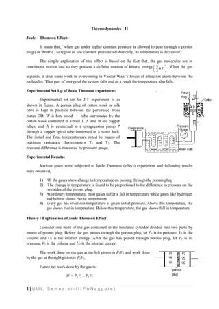
  • 1. 1 | U I I I , S e m e s t e r - I I ( P A N a g p u r e ) Thermodynamics - II Joule – Thomson Effect: It states that, “when gas under higher constant pressure is allowed to pass through a porous plug ( or throttle ) to region of low constant pressure adiabatically, its temperature is decreased.” The simple explanation of this effect is based on the fact that, the gas molecules are in continuous motion and so they possess a definite amount of kinetic energy 3 2 kT       . When the gas expands, it does some work in overcoming in Vander Waal’s forces of attraction exists between the molecules. Thus part of energy of the system falls and as a result the temperature also falls. Experimental Set Up of Joule Thomson experiment: Experimental set up for J-T experiment is as shown in figure. A porous plug of cotton wool or silk fibre is kept in position between the perforated brass plates DD. W is box wood tube surrounded by the cotton wool contained in vessel J. A and B are copper tubes, end A is connected to a compression pump P through a copper spiral tube immersed in a water bath. The initial and final temperatureare noted by means of platinum resistance thermometers T1 and T2. The pressure difference is measured by pressure guage. Experimental Results: Various gases were subjected to Joule Thomson (effect) experiment and following results were observed, 1) All the gases show change in temperature on passing through the porous plug. 2) The change in temperature is found to be proportional to the difference in pressure on the two sides of the porous plug. 3) At ordinary temperature, most gases suffer a fall in temperature while gases like hydrogen and helium shows rise in temperature. 4) Every gas has inversion temperature at given initial pressure. Above this temperature, the gas shows rise in temperature. Below this temperature, the gas shows fall in temperature. Theory / Explanation of Joule Thomson Effect: Consider one mole of the gas contained in the insulated cylinder divided into two parts by means of porous plug. Before the gas passes through the porous plug, let P1 is its pressure, V1 is the volume and U1 is the internal energy. After the gas has passed through porous plug, let P2 is its pressure, V2 is the volume and U2 is the internal energy. The work done on the gas at the left piston is P1V1 and work done by the gas at the right piston is P2V2. Hence net work done by the gas is: W = P2V2 – P1V1
  • 2. 2 | U I I I , S e m e s t e r - I I ( P A N a g p u r e ) Since the process was conducted adiabatically. Δq = 0 According to first law of thermodynamics, Δq = ΔU + W ΔU = -W Or U2 - U1 = - (P2V2 – P1V1) = P1V1 – P2V2  U1+ P1V1 = U2 + P2V2 H1 = H2 (Since, U + PV = H) Or dH = 0 Thus in this process the heat content or enthalpy (U + PV = H) of the gas remains constant. If the gas obeys Boyle’s law P1V1 = P2V2, then U2 = U1. This means that the internal energy of the gas is the same on both sides of the porous plug. But real gas obeys the law closely only at its Boyle temperature. Therefore for real gases there are three possible cases. 1) At the Boyle temperature, P1V1 = P2V2, then U2 = U1. Hence in this case temperature of the gas remains same. 2) Below the Boyle temperature, P1V1 < P2V2, then U2 < U1. Hence in this case internal energy of the gas decreases and hence there will be fall in temperature of the gas. 3) Above the Boyle temperature, P1V1 > P2V2, then U2 > U1. Hence in this case internal energy of the gas increases and hence there will be rise in temperature of the gas. Joule – Thomson coefficient: It is defined as, the ratio of change in temperature in degrees of the gas in throttle expansion (Joule Thomson expansion) to the pressure drop of one atmosphere under the condition of constant enthalpy. i,e. H dT dP        For fall in temperature of the gas  is positive, for rise in temperature  is negative. The temperature at which gas neither cools nor heats on expansion i,e. where  = 0, is called inversion point. Liquefaction of gases: In general, there are two methods of liquefaction of gases. 1) Cascade cooling and 2) Regenerative (Joule-Thomson) cooling.
  • 3. 3 | U I I I , S e m e s t e r - I I ( P A N a g p u r e ) 1) Cascade cooling: We know that, the gas cannot be liquefied until it is cooled below its critical temperature. But once this temperature has been reached, the gas can be liquefy by applying sufficient pressure. In this process gas is cooled below its critical temperature by passing it through the number of stages of volatile refrigerants of successively lower boiling points. Then by applying sufficient pressure, the gas can be liquefied. 2) Regenerative (Joule-Thomson) cooling: According to the Joule-Thomson effect, when gas under pressure is allowed to expand through porous plug, it suffers change in temperature. Similar effect is observed if constricted orifice such as nozzle is used instead of porous plug. If the initial temperature of the gas is below its inversion temperature, then on expanding through the orifice its temperature decreases. A portion of the gas thus cooled by the Joule-Thomson expansion is used to cool the other portion of the gas. Thus incoming gas is cooled by the outgoing cooled gas. By continuing this process, ultimately temperature is reached at which gas is liquefied. Liquefaction of Hydrogen Gas: The critical temperature of hydrogen is -2410 C which can not be attain by any independent cooling agent. Therefore Joule-Thomson effect is used to liquefy the hydrogen gas. The inversion temperature for an ordinary initial pressure is -800 C and its Boyle temperature is -1690 C. Therefore it is necessary to precool the gas bellow -800 C, but for appreciable cooling by means of Joule-Thomson effect it should be cooled to its Boyle temperature. The apparatus used for the liquefaction of hydrogen gas is as shown in figure. The hydrogen gas is first carefully purified so that it is free from O2, N2 and other impurities. It is compressed to pressure about 200 atmospheres and then passed through the coils as shown in figure, before it suffers throttle expansion through the valve N. In first chamber it is cooled by the surrounding solid CO2 and alcohol. In chamber A, it is further cooled by outgoing cooled hydrogen. In chamber B, it is cooled by liquid air contained in the chamber. In chamber C, it is cooled to -2080 C by liquid air boiled under reduced pressure (10 cm of Hg). Now cooled hydrogen at pressure 150 atmospheres, when passed through regenerative coil G and allowed to expand through nozzle N to pressure one atmosphere. Consequently it is further cooled due to Joule-Thomson effect.
  • 4. 4 | U I I I , S e m e s t e r - I I ( P A N a g p u r e ) The cooled hydrogen is then allowed to circulate back to the pump. This process of regenerative cooling is continues and after few cycles the temperature of the hydrogen falls to its boiling point -2530 C. It is then liquefied into Dewar flask. Liquefaction of Helium Gas: The critical temperature of helium is -2680 C and its inversion temperature for an ordinary initial pressure is - 2430 C and its Boyle temperature is -2540 C. Therefore in order to liquefy the helium gas it should be precooled to - 2540 C. The apparatus used for the liquefaction of helium gas is as shown in figure. The Helium gas is first carefully purified so that it is free the impurities. It is compressed to pressure about 40 atmospheres and then passed through the spiral tubes S1,S2, S3 and S4 as shown in figure. In the spiral tube S1 and S3 the gas cooled to -258C by liquid hydrogen boiling under reduced pressure in chamber E. in the spiral tubes S2 and S4, it is cooled by outgoing cooled helium. At the nozzle N the cooled helium at -2580 C suffers throttle expansion. Consequently it is further cooled due to Joule-Thomson effect. After few cycles the temperature of the helium is reached to its boiling point and it is liquefied in chamber F.
  • 5. 5 | U I I I , S e m e s t e r - I I ( P A N a g p u r e ) Maxwell’s Thermodynamic Relations Thermodynamic Variables: The thermodynamic state of a system is specified by some of its properties like pressure, temperature, volume, internal energy, entropy. These properties undergo a change when system passes from one state to another. These variables are known as thermodynamic variables or co- ordinates. These are macroscopic variables. Extensive Variable: An extensive variable of a system is macroscopic parameter which describes system in equilibrium and which has value equal to sum of its values in all part of the system. The extensive variable depends on mass and size of the substance present in the system. For example: volume, mass, internal energy, entropy, length, area, heat capacity, electric charge, etc. Intensive Variable: An intensive variable of a system is macroscopic parameter which describes system in equilibrium and which has same value in all part of the system. The intensive variable is independent on mass and size of the substance present in the system. For example: pressure, temperature, density, surface tension, viscosity, refractive index, etc. Consider a homogeneous system in equilibrium. Suppose system is divided into many parts. If x is the macroscopic variable of the system and has values x1, x2, x3,…… in each part of the system, then x = x1 + x2 + x3 +………. if x is extensive variable; x = x1 = x2 = x3 =………. if x is intensive variable; Maxwell’s Thermodynamic Relations: From the first and second law of thermodynamics, Maxwell was able to derive four fundamental thermodynamic relations. According to first law of thermodynamics, we have Q dU W   as W PdV  Q dU PdV   …… (1) According to second law of thermodynamics, we have Q TdS  …… (2) From eq 1 and eq 2, we have TdS dU PdV  Or dU TdS PdV  ……. (3) Let U, S and V are the functions of two independent variables i.e. ( , ), ( , ) & ( , )U U x y S S x y V V x y  
  • 6. 6 | U I I I , S e m e s t e r - I I ( P A N a g p u r e ) y x U U dU dx dy x y               ….. (4) y x S S dS dx dy x y              ….. (5) y x V V dV dx dy x y              ….. (6) Using eq 4,5 &6 in eq 3, we have y y yx x x U U S S V V dx dy T dx T dy P dx P dy x y x y x y                                                Equating coefficients of dx and dy, we have y y y U S V T P x x x                         ….. (7) x x x U S V T P y y y                        ….. (8) Differentiating eq 7 w.r.t. y and eq 8 w.r.t. x U S T S V P V T P y x y x y x y x y x                                                             ….. (9) U S T S V P V T P x y x y x y x y x y                                                             ….. (10) As dU is perfect differential, therefore U y x         = U x y        S T S V P V S T S V P V T P T P y x y x y x y x x y x y x y x y                                                                                                          Also dS & dV are perfect differential, therefore and S S V V y x x y y x x y                                     Above eq becomes T S P V T S P V y x y x x y x y                                                             …… (11) This is Maxwell’s general thermodynamic equation. 1) Let x =S and y=V, therefore from eq 11, we have T S P V T S P V V S V S S V S V                                                     as 0 V S S V                and 1 S V S V                S V T P V S                 This is known as Maxwell’s first thermodynamic relation. 2) Let x =T and y=V, therefore from eq 11, we have
  • 7. 7 | U I I I , S e m e s t e r - I I ( P A N a g p u r e ) T S P V T S P V V T V T T V T V                                                     as 0 T V V T                and 1 T V T V                T V S P V T                This is known as Maxwell’s second thermodynamic relation. 3) Let x =S and y=P, therefore from eq 11, we have T S P V T S P V P S P S S P S P                                                     as 0 P S S P                and 1 S P S P                S P T V P S                This is known as Maxwell’s third thermodynamic relation. 4) Let x =T and y=P, therefore from eq 11, we have T S P V T S P V P T P T T P T P                                                     as 0 T P P T                and 1 T P T P                T P S V P T                This is known as Maxwell’s fourth thermodynamic relation. Thermodynamic Potentials: There are four thermodynamic potentials i) Internal energy, U ii) Helmholtz free energy, F=U – TS iii) Enthalpy, H=U + PV iv) Gibbs free energy, G = U – TS + PV 1. Internal energy, U : The internal energy is the total en energy of a system. It is called first thermodynamic potential. According to combined form of first and second law of thermodynamics dU = TdS – PdV This equation gives change in internal energy in terms of four state variables P, V, T & S. For an isochoric-adiabatic process: dV = 0 and dQ = 0 dU = 0 or U is constant. 2. Helmholtz free energy, F: It is defined as F=U – TS As U, T & S are state variables, F is also state variable. It has dimensions of energy. ( )dF dU d TS dF dU TdS SdT       
  • 8. 8 | U I I I , S e m e s t e r - I I ( P A N a g p u r e ) As dU = TdS – PdV dF PdV SdT    For an isochoric-isothermal process: dV = 0 and dT = 0 0 or is constant.dF F  3. Enthalpy, H: It is defined as H=U + PV As U, P & V are state variables, H is also state variable. It has dimensions of energy. ( )dH dU d PV dH dU PdV VdP        As dU = TdS – PdV dH TdS VdP   For an isobaric-adiabatic process process: dP = 0 and dQ = TdS = 0 0dH  or H is constant 4. Gibbs free energy, G: It is defined as G=U + PV – TS As U, P, V, T & S are state variables, G is also state variable. It has dimensions of energy. ( ) ( )dG dU d PV d TS dG dU PdV VdP TdS SdT           As dU = TdS – PdV dG VdP SdT   For an isobaric-isothermal process process: dP = 0 and dT = 0 0dG  or G is constant Significance of Thermodynamic Potentials: A mechanical system is said to be in stable equilibrium when potential energy of the system is minimum. It means that the system must proceeds in such a direction so as to acquire minimum potential energy. In thermodynamics, the behavior of U, F, H & G is similar to potential energy in mechanics. As the direction of isochoric –isothermal process is to make F minimum, the direction of isobaric –adiabatic process is to make H minimum and the direction of isobaric –isothermal process is to make G minimum. Since four functions U, F, H & G play same role in thermodynamics as played by potential energy in mechanics, hence they are called thermodynamic potentials. Applications of Maxwell’s Thermodynamic Relations: 1. Joule Thomson effect: We know that in Joule Thomson expansion enthalpy of the gas remains constant i.e. H=U + PV = constant ( ) 0 0 dH dU d PV dH dU PdV VdP          As dU = TdS – PdV
  • 9. 9 | U I I I , S e m e s t e r - I I ( P A N a g p u r e ) 0dH TdS VdP    Now dS being perfect differential and S is a function of P and T i.e. S = f(P,T), we have P T S S dS dT dP T P                Substituting in above equation 0 P T S S T dT T dP VdP T P                  0 P T S S T dT T V dP T P                    0 P T Q S dT T V dP T P                    As P P P S Q T C T T                P T S C dT T V dP P            According to Maxwell’s fourth relation T P S V P T                P P V C dT T V dP T           1 PP dT V T V dP C T           As H dT dP         is Joule Thomson coefficient 1 PP V T V C T            2. Clausius - Clapeyron Latent Heat Equation: Maxwell’s second thermodynamic relation is given by T V S P V T                From the second law of thermodynamics 𝜕𝑆 = 𝜕𝑄 𝑇 ∴ 1 𝑇 ( 𝜕𝑄 𝜕𝑉 ) 𝑇 = ( 𝜕𝑃 𝜕𝑇 ) 𝑉 ∴ ( 𝜕𝑄 𝜕𝑉 ) 𝑇 = 𝑇 ( 𝜕𝑃 𝜕𝑇 ) 𝑉
  • 10. 10 | U I I I , S e m e s t e r - I I ( P A N a g p u r e ) This equation shows that the heat absorbed per unit increase in volume at constant temperature is equal to the product of the absolute temperature and rate of increase of pressure per unit increase in temperature at constant volume. Let L be the latent heat of fusion (or vaporization) of the substance. Let V1 & V2 be the specific volumes of the substance at its melting temperature (or boiling temperature). i.e. ( 𝜕𝑄 𝜕𝑉 ) 𝑇 = 𝐿 𝑉2 − 𝑉1 From above equations we have ( 𝜕𝑃 𝜕𝑇 ) 𝑉 = 𝐿 𝑇(𝑉2 − 𝑉1) This is called Clausius - Clapeyron latent heat equation.