Risi ottavio

Time Series Analysis Project, Dec 2017
QUESTION 1
The analysis starts with the observation of time series of variables gdp, infl and rate (growth rate of the
gdp, inflation rate and policy interest rate). Their graphs show persistence and ergodicity and they fluctuate
around ‘0’, that seems their mean (the processes are mean-reverting - Figure 1). Table 1 shows all the
descriptive statics of three variables: all their means are practically ‘0’ and all mean square errors are very
low. Now the objective is to confirm stationarity of each time series in order to estimate a VAR model in a
multivariate way. The first test is the ADF, done for each variable, his null hypothesis is: process has a unit
root. Indeed, a unit root in the process compromises the stationarity, and the estimate of a VAR model
becomes difficulty. For gdp the ADF test, done without a constant because it is ‘0’ (μ = 0), rejects the null
hypothesis with a p-value < 0,001 (Table 2). For the same test infl and rate, always without constant (μ = 0),
result stationary too, thanks to their very low p-values (Table 3 – 4). The second test is the KPSS, done for
each variable, it’s another way to confirm stationarity. Indeed, its null hypothesis is: process is stationary.
Gdp, infl and rate pass this test for all the critical values (10% - 5% - 1%), it is another confirm they are
stationary. So, to proceed it’s not necessary to take differences of variables. From three univariate
processes, we move to the multivariate one estimating the reduced form VAR(p). Information criteria
Akaike (AIC) and Schwartz (BIC) suggest the right order p of the reduced VAR(p). In this case 1 is the order
suggested by all criteria (Figure 2), the smallest value for AIC and BIC. Now the reduced form of VAR(1) can
be estimated (stars represent the level of significance 1%∗∗∗
5%∗∗
10%∗
) :
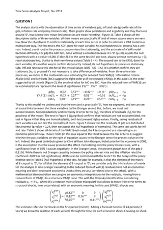
𝑉𝐴𝑅(1):
𝑔𝑑𝑝𝑡
𝑖𝑛𝑓𝑙 𝑡
𝑟𝑎𝑡𝑒𝑡
=
0,02
0,03
0,02∗
+
0,52∗∗∗ −0,32∗∗∗ −0,11∗
0,27∗∗∗
0,51∗∗∗
−0,01
0,19∗∗∗
0,28∗∗∗
0,53∗∗∗
𝑔𝑑𝑝𝑡−1
𝑖𝑛𝑓𝑙 𝑡−1
𝑟𝑎𝑡𝑒𝑡−1
+
𝜀1𝑡
𝜀2𝑡
𝜀3𝑡
Thanks to this model we understand that the constant is practically ‘0’, how we expected, and we can see
all causal links between the three variables (in the Granger sense). But, before, we must test
autocorrelation, homoskedasticity and normality of error terms (𝜀𝑡), therefore of residuals (𝜀𝑡̂), for the
goodness of the model. The test in Figure 3 (Ljung-Box) confirms that residuals are not autocorrelated, the
test in Figure 4 that they are homoskedastic, both test present high p-values. Finally, saving residuals of
each variables we can test the normality of them. Figure 5 shows that the residuals of gdp are distributed
like a normal (p-value = 0,24, then we accept the null hypothesis of normality). The same test works for infl
and rate. Table 5 shows all details of the VAR(1) estimated, the F test reported are interesting in an
economic point of view. These F tests (in this case equal to the t test because the Var order is 1) suggest
whether the past variables on the right of equation causes in the Granger sense the present value on the
left. Indeed, the great contribute given by Clive William John Granger, Nobel prize for the economy in 2003,
is the assumption that the cause preceded the effect. Considering only the policy interest rate, with a
significance level of 10% it causes negatively, in the Granger sense, the present growth rate of the gdp (-
0,11%). While there is not Granger causality between the policy interest rate and the inflation rate (the
coefficient -0,01% is not significative). All this can be confirmed with the tests F for the delays of the policy
interest rate in Table 5 (null hypothesis of the test, for gdp for example, is that the element of the matrix
a13 is equal to ‘0’, for infl that the element a23 is equal to ‘0’; we consider only the third column of matrix
for the analysis of rate Granger causality). In the reduced form of VAR(1) residuals have not an economics
meaning and don’t represent economics shocks (they are also correlated one to the other). With a
mathematical demonstration we can give an economics interpretation to the residuals, moving from a
reduced form of VAR(1) to a structural VAR(1) one. This with the Cholesky Identification, considering
residuals 𝜀𝑡 = 𝐵𝑢 𝑡, where B is a rotation matrix (lower triangular) that allows to move from error terms to
structural shocks, now uncorrelated, with an economic meaning. In this case SVAR(1) shocks are:
(
𝜀𝑡
𝑔𝑑𝑝
𝜀𝑡
𝑖𝑛𝑓𝑙
𝜀𝑡
𝑟𝑎𝑡𝑒
) = (
0,42∗∗∗
0 0
0,12∗∗∗
0,36∗∗∗
0
0,25∗∗∗
0 0,11∗∗∗
) (
𝑢 𝑡
𝑔𝑑𝑝
𝑢 𝑡
𝑖𝑛𝑓𝑙
𝑢 𝑡
𝑟𝑎𝑡𝑒
)
This estimate refers to the shocks in the first period (month). Adding a forecast horizon of 24 periods (2
years) we know the reaction of each variable through the time for each economic shock. Focusing on shock

of the interest rate (variable rate), therefore the transmission mechanism of the monetary policy, Table 5
shows the reaction of the growth rate of gdp and the inflation rate through 24 periods (2 years).
In a dynamic point of view the impulse response functions (IRF) of a shock in the interest rate causes these
effects in gdp and infl in 2 years:
These graphs are useful to understand the transmission mechanism of the monetary policy, using the
interest rate shock (𝑢 𝑡
𝑟𝑎𝑡𝑒
). The first graph demonstrates that a sudden restrictive monetary policy (interest
rate increase – shock) doesn’t influence the growth rate of gdp in the first month (how we have evaluated
in SVAR(1)), but only after a month. Indeed, after a month the growth rate of gdp falls by 2% and after 11
months (about 1 year) it restores gradually the value before the shock. This dynamic transmission of the
shock is confirmed by the economic theory. Indeed, an increase of the interest rate reduces the liquidity in
the system, so the demand decreases and gdp too. But the response of gdp is temporarily and not instant.
As the second graph, it demonstrates a particular relationship between the shock in the interest rate and
the inflation rate. Also in this case inflation rate reacts to the shock of the interest rate after a month (how
we expected), precisely it falls by 0,006% after three months. So, the inflation returns gradually to its initial
value after 13 months (about 1 year). But this impact on inflation rate is small and not statistically
significant, how demonstrated by the confidence interval at 95% (green cloud) that covers entirely the ‘0’
line. The result of this estimate is that interest rate shock practically doesn’t influence inflation rate.
However, using economic theory and forcing the statistic estimate (for example considering only the red
line of the graph), we can assert a delayed and negative relationship between the shock of the interest rate
and the inflation rate. Indeed, during a restrictive monetary policy the demand falls and consequently the
level of prices drops with delay.
Finally, a right ARMA(p;q) model for the interest rate can be selected analysing its correlogram in Figure 6.
The correlogram suggests a model AR(p) pure, since the total sample autocorrelations (first part in Figure 6
ACF) come down gradually, while the partial ones (second part in Figure 6 PACF) stop brusquely in the
second delay. The AIC and BIC criteria (Table 7 for all analysis of the right ARMA model) confirm an
ARMA(2;0), without a constant (μ=0). Indeed, all parameters are 1% significative (green numbers of Table 7
are not 1% significative) and BIC is the smallest 184,06. This model was in competition with an ARMA(2;1)
that has the smallest AIC (171,9), but not all parameters are 1% significant. Moreover, AIC criterion doesn’t
penalize extra parameters like the BIC one. So, we maintain the AR(2). Another confirmation comes by the
Ljung-Box test (Q in Table 7) that with 12 delays presents a p-value =0,48 > 5%. We can accept the null
hypothesis of absence of autocorrelation. Already an ARMA(2;4) appears over parametrized, so we can
stop there. 𝐴𝑅(2): 𝑟𝑎𝑡𝑒𝑡 = 0,95∗∗∗
𝑟𝑎𝑡𝑒𝑡−1 − 0,22∗∗∗
𝑟𝑎𝑡𝑒𝑡−2 + 𝜀𝑡
The main difference between an ARMA and VAR model is that the first is a stochastic univariate process
that explains the dynamic of a single variable; the second is a multivariate stochastic process that considers
the dynamic of a vector of variables, then their simultaneous responses (in fact the arrangement of
variables in the matrix is fundamental). In both models we can estimate the response impulse function of
variables to unexpected shocks (𝜀𝑡), which persist because of the persistence of the models. The difference
is that the VAR model gives precise economic signals about the response of an economic variable to the
shock of the other.

QUESTION 2:
The money demand function is: 𝑚 = 𝛽0 + 𝛽1 𝑦 − 𝛽2 𝑖 where m is the quantity of money, y the gross
domestic product and i the short-term interest rate. It represents a long run equilibrium. Analysing data
(Figure 7), we understand that m and y are RW which share a trend, also the variable i is a RW stochastic
process and, like the others, needs to the fist difference to be stationary (m, y, i ̴ I(1)). However, the three
not stationary variables together become stationary, in a long run equilibrium (spurious correlation). The
confirm of this assertion comes by the Engle-Granger test, which tests the stationarity of residuals of the
money demand function (𝑧𝑡 = 𝑚 𝑡 − 𝛽0 − 𝛽1 𝑦𝑡 + 𝛽2 𝑖 𝑡 ̴ 𝐼(0)). The test in Table 8 confirms cointegration,
indeed the variables m, y, i have a unit root, while their residuals not (p-values analysis). Then the
cointegration regression is 𝑚 𝑡 = −0,25 + 0,96∗∗∗
𝑦𝑡 − 0,29∗∗∗
𝑖 𝑡 , all coefficients are super consistence
(they converge in a point) and this money demand function estimated represent a long run equilibrium
(high 𝑅2
= 0,99). The residuals of this cointegration regression, which fluctuate around ‘0’ (𝐸(𝑧𝑡) = 0
Figure 8), can be consider the equilibrium errors (disequilibria from the cointegrating relation). They
capture the deviations from equilibrium and, in this case, are: 𝑧𝑡 = 𝑚 𝑡 + 0,25 − 0,96𝑦𝑡 + 0,29𝑖 𝑡 .
To verify if and which variables react to the disequilibrium from the cointegrating relation, we can use the
error correction mechanism (ECM Figure 10), estimating an OLS for each variable:
𝑑𝑖𝑓𝑓𝑚 𝑡 = 0,06 𝑑𝑖𝑓𝑓𝑦𝑡−1 − 0,03𝑑𝑖𝑓𝑓𝑖 𝑡−1 − 0,03𝑑𝑖𝑓𝑓𝑚 𝑡−1 − 0,29∗∗∗
𝑧𝑡−1
𝑑𝑖𝑓𝑓𝑖 𝑡 = −0,05𝑑𝑖𝑓𝑓𝑦𝑡−1 − 0,05𝑑𝑖𝑓𝑓𝑖 𝑡−1 + 0,01𝑑𝑖𝑓𝑓𝑚 𝑡−1 + 0,15∗∗∗ 𝑧𝑡−1
𝑑𝑖𝑓𝑓𝑦𝑡 = −0,04𝑑𝑖𝑓𝑓𝑦𝑡−1 + 0,002𝑑𝑖𝑓𝑓𝑖 𝑡−1 + 0,04𝑑𝑖𝑓𝑓𝑚 𝑡−1 + 0,002𝑧𝑡−1
The dependent variable is the first difference (all variables are difference-stationary DS), on the right the
first three variables represent the short run dynamic, while the coefficient of the delayed residuals captures
how the system restores the equilibrium of the money demand function (in equilibrium 𝑧𝑡 = 𝑧𝑡−1 = 0).
The variables that react to the disequilibrium are those that have the coefficient (𝛾) of the delayed
residuals significative (1%∗∗∗
). Then the quantity of money and the short-term interest rate react to the
disequilibrium, while the gross domestic product is weakly exogenous. Precisely, being 𝑧𝑡−1 = 𝑚 𝑡−1 +
0,25 − 0,96𝑦𝑡−1 + 0,29𝑖 𝑡−1 , we can analyse all reaction of m and i for restoring the initial equilibrium. For
the quantity of money: if in t-1 the interest rate rises, in t the equilibrium is restored with a decrease of the
money quantity; if in t-1 the gross domestic product rises, in t the equilibrium is restored with an increase
of the money quantity. For the short-term interest rate: if in t-1 money quantity rises, in t the equilibrium is
restored with an increase of the interest rate; if in t-1 gross domestic product rises, in t the equilibrium is
restored with a decrease of the interest rate. All this is confirmed by the macroeconomic theory, indeed the
equation in the Question 2 represents the long run equilibrium in the money and financial activities market
(LM curve). In equilibrium the money supply is equal to the money demand. A shock of a variable in the
equation (disequilibrium) creates a response of the endogenous variables money quantity (m) and short-
term interest rate (i), ruled by the Central Bank. While the dynamics of the gross domestic product is
weakly exogenous. In the model 𝛽1 represents the money demand sensitivity to change in income (gdp),
while 𝛽2 the money demand sensitivity to change in short-term interest rate (this relation is negative).
In a multivariate way, all this analysis can be done with a VECM model. It’s useful to derivate, using the
Cholesky identification seen in the first question, the impulse response function of dependent variables for
restoring the long run equilibrium caused by a momentary disequilibrium (shock of a variable). Using the
same dataset, we can estimate a VECM model: the coefficients are practically similar and m and i are the
only ones that react to the disequilibrium (like before). The four dynamics seen of the economic variables
are also confirmed by the impulse response functions (below is considered only one of the three reactions
of each dependent value, complete graph in Figure 9 – y confirms to be weakly exogenous: 95% conf. int.
hides the ‘0’ line):

APPENDIX
Figura 1: gdp, infl and rate time series
Variabile Media Mediana SQM Min Max
gdp -0,0116 -0,0115 0,507 -1,36 1,44
infl 0,0460 0,0516 0,483 -1,18 1,36
rate 0,0736 0,0727 0,481 -1,37 1,47
Tabella 1: descriptive statics time series

Tabella 2: ADF test for gdp
Tabella 3: ADF test for infl
Tabella 4: ADF test for rate

Figura 2: information criteria for Var(p)
Figura 3: test autocorellation residuals Var(1)

Figura 4: test homoskedasticity Var(1)
Figura 5: test normality residuals of gdp in Var(1)

Equazione 1: gdp
Errori standard HAC, larghezza di banda 5 (Kernel di Bartlett)
Coefficiente Errore Std. rapporto t p-value
const 0,0164368 0,0213894 0,7685 0,4427
gdp_1 0,524043 0,0423524 12,37 <0,0001 ***
infl_1 −0,318480 0,0550883 −5,781 <0,0001 ***
rate_1 −0,105248 0,0610948 −1,723 0,0857 *
Somma quadr. residui 71,18443 E.S. della regressione 0,424516
R-quadro 0,305357 R-quadro corretto 0,300081
F(3, 395) 63,35728 P-value(F) 1,83e-33
rho 0,018480 Durbin-Watson 1,961943
Test F per zero vincoli:
Tutti i ritardi di gdp F(1, 395) = 153,1 [0,0000]
Tutti i ritardi di infl F(1, 395) = 33,423 [0,0000]
Tutti i ritardi di rate F(1, 395) = 2,9677 [0,0857]
Equazione 2: infl
const 0,0270280 0,0188617 1,433 0,1527
gdp_1 0,270517 0,0378944 7,139 <0,0001 ***
infl_1 0,511354 0,0476192 10,74 <0,0001 ***
rate_1 −0,0142334 0,0523867 −0,2717 0,7860
F(3, 395) 97,63396 P-value(F) 2,71e-47
Equazione 3: rate
const 0,0238105 0,0141124 1,687 0,0924 *
gdp_1 0,192287 0,0284596 6,756 <0,0001 ***
infl_1 0,279202 0,0333280 8,377 <0,0001 ***
rate_1 0,527889 0,0376379 14,03 <0,0001 ***
F(3, 395) 276,3990 P-value(F) 1,24e-96
Tabella 5: Var(1) estimated

Month Gdp Infl Rate
Tabella 6:analytics IRF rate 24 months

Figura 6: correlogram rate
ARMA(1,0) ARMA(2,0) ARMA(1,1) ARMA(2,1) ARMA(2,4)
θ1 0,78 0,95 0,69 1,31 -0,49
θ2 -0,22 -0,5 0,47
α1 0,24 -0,39 1,43
α2 0,68
α3 0,38
α4 0,16
Q 30,38 9,59 12,15 7,22 7,01
p-value 0,001 0,48 0,28 0,61 0,32
AIC 189,29 172,08 174,84 171,9 175,81
BIC 197,27 184,06 186,82 187,86 203,75
Tabella 7:analysis ARMA models for rate

Figura 7: dynamic variables m, y. i
Passo 1: test per una radice unitaria in m
Test Dickey-Fuller aumentato per m
test all'indietro da 12 ritardi, criterio AIC
Ampiezza campionaria 399
Ipotesi nulla di radice unitaria: a = 1
Test con costante
inclusi 0 ritardi di (1-L)m
Modello: (1-L)y = b0 + (a-1)*y(-1) + e
Valore stimato di (a - 1): 0,00112703
Statistica test: tau_c(1) = 0,567808
p-value 0,9887
Passo 2: test per una radice unitaria in y
Test Dickey-Fuller aumentato per y
Test con costante
incluso un ritardo di (1-L)y
Modello: (1-L)y = b0 + (a-1)*y(-1) + ... + e
Valore stimato di (a - 1): -0,000965234
Statistica test: tau_c(1) = -0,441053
p-value asintotico 0,8998

Passo 3: test per una radice unitaria in i
Test Dickey-Fuller aumentato per i
Test con costante
inclusi 0 ritardi di (1-L)i
Modello: (1-L)y = b0 + (a-1)*y(-1) + e
Valore stimato di (a - 1): 0,00298417
Statistica test: tau_c(1) = 0,973453
p-value 0,9964
Passo 4: regressione di cointegrazione
Regressione di cointegrazione -
OLS, usando le osservazioni 1973:01-2006:04 (T = 400)
Variabile dipendente: m
coefficiente errore std. rapporto t p-value
--------------------------------------------------------------
const −0,254378 0,611615 −0,4159 0,6777
y 0,956123 0,0155740 61,39 9,32e-205 ***
i −0,294614 0,00994982 −29,61 1,53e-102 ***
Media var. dipendente 97,48300 SQM var. dipendente 59,21247
Log-verosimiglianza −1143,329 Criterio di Akaike 2292,658
Criterio di Schwarz 2304,633 Hannan-Quinn 2297,400
Passo 5: test per una radice unitaria in uhat
Test Dickey-Fuller aumentato per uhat
Modello: (1-L)y = (a-1)*y(-1) + ... + e
Valore stimato di (a - 1): -0,279877
Statistica test: tau_c(3) = -6,39466
p-value asintotico 1,505e-007
Coefficiente di autocorrelazione del prim'ordine per e: 0,010
differenze ritardate: F(4, 390) = 2,225 [0,0657]
Tabella 8: Engle-Granger test for cointegration

Figura 8: residuals money demand function estimated
Figura 9: impulse response function VECM

Figura 10: regressions ECM

Risi ottavio

Recommended

Recommended

More Related Content

What's hot

What's hot (20)

Similar to Risi ottavio

Similar to Risi ottavio (20)

Recently uploaded

Recently uploaded (20)

Risi ottavio