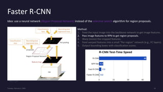
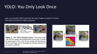
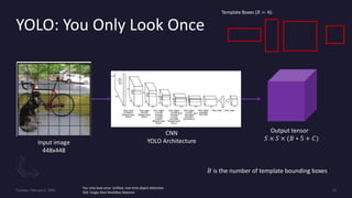
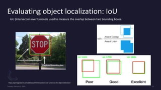
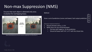
This document provides an overview of object detection using convolutional neural networks (CNNs). It discusses why CNNs are well-suited for object detection, defines object detection, and describes several popular CNN-based object detection algorithms including R-CNN, Fast R-CNN, Faster R-CNN, and YOLO. It also covers important object detection concepts like region proposals, sliding windows, IoU for evaluating localization accuracy, and NMS for removing overlapping detections. Open-source resources for implementing these algorithms are also provided.
2. Agenda
Sample Footer Text
Why CNNs?
What is a CNN?
Object Detection: Definition
Sliding Windows Detection
Region Proposals
R-CNN
Fast R-CNN
Faster R-CNN
YOLO
IoU
NMS
Open-Source Resources
Variables of object detection
Next Steps
4. What is a CNN?
Activation map
Input image
Applying many
filters
That’s it! A full convolutional layer.
A representation of the image.
https://analyticsindiamag.com/convolutional-neural-network-image-classification-overview/
Filter (3x3)
5. Object Detection: Definition
CNN
RGB
Image
List of objects
Output
Input
For each object:
1. Category label (person, car, cat, …)
2. Bounding box
(𝑥, 𝑦)
𝑊𝑖𝑑𝑡ℎ
𝐻𝑒𝑖𝑔ℎ𝑡
What is in the image and where is it?
6. Sliding Windows Detection
CNN
Is there a car in the image?
1
CNN 0
Issue? Huge computational cost
OverFeat: Integrated Recognition, Localization and Detection using Convolutional Networks https://arxiv.org/pdf/1312.6229v4.pdf
8. R-CNN: Region-Based CNN
Proposed
regions
(~2K)
Warped
image
regions
224x224
Rich feature hierarchies for accurate object detection and semantic segmentation.
Method:
1. Run selective search to get ~2K regions.
2. Resize (warp) regions to 224x224
3. Run regions independently through a CNN.
4. Linear SVM (FC layers)
What if regions do not exactly match the object?
Solution: CNN should learn to output a transformation of the Bbox size.
Caveat: CNNs share weights!
Issues?
1. Very slow! Run ~2k forward passes per image.
2. Using the selective search to select image regions. There is no learning at that stage.
9. Fast R-CNN
Idea: swap the order of the CNN with the warping.
Method:
1. Feed the input image into a CNN and compute feature maps.
2. Run the selective search on feature maps. “Cropping”
3. Warp (resize) the cropped features.
4. Feed warped features into a small “Per-region” network (e.g., FC layers).
5. Output bounding boxes with classification scores.
10. Faster R-CNN
Idea: use a neural network (Region Proposal Network) instead of the selective search algorithm for region proposals.
Method:
1. Feed the input image into the backbone network to get image features.
2. Pass image features to RPN to get region proposals.
3. Warp (resize) the cropped features.
4. Feed warped features into a small “Per-region” network (e.g., FC layers).
5. Output bounding boxes with classification scores.
11. YOLO: You Only Look Once
You only look once: Unified, real-time object detection
SSD: Single-Shot MultiBox Detector
Idea: use one giant CNN to go from the input image to a tensor of scores.
Eliminates the need for region proposals.
12. YOLO: You Only Look Once
You only look once: Unified, real-time object detection
SSD: Single-Shot MultiBox Detector
Input image
448x448
CNN
YOLO Architecture
Output tensor
𝑆 × 𝑆 × (𝐵 ∗ 5 + 𝐶)
𝐵 is the number of template bounding boxes
Template Boxes (𝐵 = 4):
13. Evaluating object localization: IoU
IoU (Intersection over Union) is used to measure the overlap between two bounding boxes.
https://pyimagesearch.com/2016/11/07/intersection-over-union-iou-for-object-detection/
14. Non-max Suppression (NMS)
Ensures that each object is detected only once.
A solution for overlapping boxes.
Method:
Given a set of predictions (scores and boxes). Each output prediction:
𝑝𝑐
𝑏𝑥
𝑏𝑦
𝑏ℎ
𝑏𝑤
(Greedy Implementation)
1. Discard all boxes with 𝑝𝑐 ≤ 0.6
2. While there are any remaining boxes:
• Pick box with largest 𝑝𝑐 as the prediction.
• Discard all boxes with 𝐼𝑜𝑈 ≥ 0.7 with the chosen box.
https://towardsdatascience.com/non-maximum-suppression-nms-93ce178e177c
Progression of object detection on the PASCAL VOC dataset, up until 2012 the performance almost plateaued but in 2013 when deep Convnets were being used in OD, the performance shot up pretty quickly.
Challenges:
Multiple outputs: need to output variable numbers of objects per image.
Multiple types of output: need to predict “what” (category label) as well as “where” (bounding box)
Large images: classification works at 224x224; need higher resolution for detection, often ~800x600
Objects can appear in different sizes and aspect ratios in the same image
The hope is that there will be a window containing a car in which the Convnet can detect the car in.
Disadvantage: (Slow)
- You are taking so many crops of the image and feeding each of them independently through a CNN.
Trying different window sizes. Using a larger stride can reduce the number of crops but coarser granularity can hurt performance.
Convolutional implementation:
- Pass the original image and a CNN and make a prediction of all crops at the same time.
Rather than covering all possible boxes in the image, we can reduce the number of boxes by smartly selecting a small set of those crops.
Often based on heuristics: e.g. look for “blob-like” image regions.
Relatively fast to run; e.g. Selective Search gives 2000 region proposals in a few seconds on CPU.
The idea of region proposals was the stepping-stone of many advanced object detectors such as R-CNN.
One of the most influential papers in deep learning.
All ConvNets share weights. Infeasible to train 2000 independent CNNs and it wouldn’t make sense because all of them share the same optimization goal which is to perform well on image regions.
CNNs are trained on image regions (is given a batch of image regions @ training time) from same image across different images. An classification score and a bounding box is the output of each region.
Steps:
Run selective search => gives us 2K proposed regions (which can be of different sizes and aspect ratios)
Warp (affine image warping) all regions into a fixed size (224x224; this size is a hyperparameter)
Run regions independently through a CNN which outputs the classification over C+1 categories (C defined classes and 1 unknown; a background region with no object)
Why warp? Region proposals are of different size and aspect ratio.
Transform is log-space scale transform
@ Test time: If the classification score is above a chosen threshold, we output the box, ow we don’t. Ex. If you don’t care about the categories output 10 boxes that have the lowest background score.
Problem: What if region proposals do not exactly match up to the objects in the image? Output a bounding box. The CNN outputs a transformation that transforms the region proposal box into the final output box that we want (that contains the object. we are modifying the region proposal bounding box to fit the object.
We don’t input the location of the box for the CNN to learn because we want the prediction to be invariant to the location of the object in the image.
10x times faster than R-CNN.
Per-region networks are usually part of the backbone network. E.g., if AlexNet, the backbone would be the conv layers and the per-region network would be the FC layers at the end.
Copping features Rol Pool. Idea: project region proposals extracted from the input image to the corresponding feature maps. Because we have CNN feature maps, then we know that each point in the feature maps corresponds to points in the input image.
Then Snap to grid cells (divide into 2x2 grid of equal subregions) then max-pool with each subregion.
Region features always have the same size even if input regions have different sizes!
Run image into backbone network to get image features.
Pass image features to the region proposal network to get region proposals. (rest is the same as before at this point)
Crop and resize
Per-region network
Bbox and class scores.
Faster R-CNN is 10x times faster than Fast R-CNN
Figure 2: The Model. Our system models detection as a regression problem. It divides the image into an S × S grid and for each grid cell predicts B bounding boxes, confidence for those boxes, and C class probabilities. These predictions are encoded as an S × S × (B ∗ 5 + C) tensor.
An input image is divided into multiple grid cells.
For each grid, a vector is generated through the CNN which contains the classification score and the bounding box information.
YOLO uses the idea of anchor boxes, where a multiple template boxes encompassing different sizes and shapes of objects possible to encounter in the dataset are used in training. The CNN would output a prediction for each of these template boxes. The prediction would match one of the available boxes
SxS is the number of grid cells
B is the number of bounding boxes. We multiply by 5 because for each box we output x,y (center), width, height,, and confidence score (IoU between the predicted box and ground truth box).
C is the classification score.
Within each grid cell:
Regression from each of the B boxes to a final box with 5 numbers (dx, dy, dh, dw, confidence)
Predict scores for each class (including background,.
The confidence is the measure of how much we are sure the object matches this particular template box.
Jaccard similarity (Jaccard Index) but for OD it is called IoU
A mechanism to compare two bounding boxes to evaluate our predictions.
In practice above 0.7 is good and 0.9 is as good as it can ever get.
> 0.5 decent
> 0.7 good
> 0.9 Excellent
Algorithms usually output multiple detections of the same object, which means we have multiple overlapping boxes.
If an object is detected multiple times, NMS is used to choose the best box. NMS is a method to ensure that each object is detected only once.
1. Get rid of low-probability predictions