The sampling design process

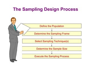
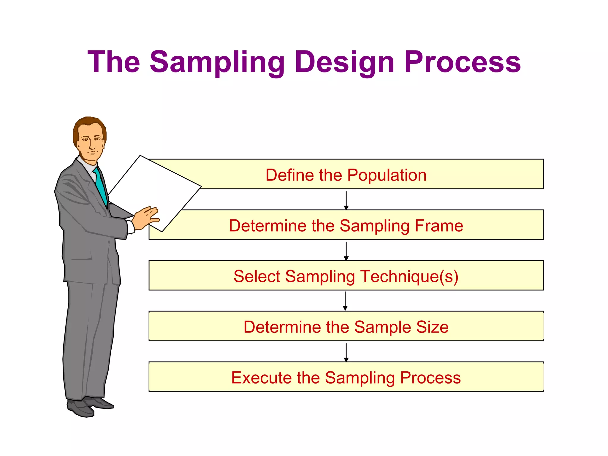
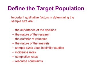
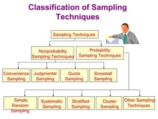
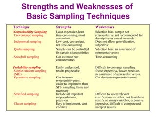
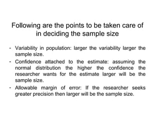
1. The Sampling Design Process
Define the Population
Determine the Sampling Frame
Select Sampling Technique(s)
Determine the Sample Size
Execute the Sampling Process

2. Define the Target Population
The target population is the collection of elements or
objects that possess the information sought by the
researcher and about which inferences are to be made.
The target population should be defined in terms of
elements, sampling units, extent, and time.
– An element is the object about which or from which
the information is desired, e.g., the respondent.
– A sampling unit is an element, or a unit containing
the element, that is available for selection at some
stage of the sampling process.
– Extent refers to the geographical boundaries.
– Time is the time period under consideration.

3. Define the Target Population
Important qualitative factors in determining the
sample size are:
– the importance of the decision
– the nature of the research
– the number of variables
– the nature of the analysis
– sample sizes used in similar studies
– incidence rates
– completion rates
– resource constraints

4. Classification of Sampling
Techniques
Sampling Techniques
Nonprobability
Sampling Techniques
Probability
Sampling Techniques
Convenience
Sampling
Judgmental
Sampling
Quota
Sampling
Snowball
Sampling
Systematic
Sampling
Stratified
Sampling
Cluster
Sampling
Other Sampling
Techniques
Simple
Random
Sampling

5. Convenience Sampling
Convenience sampling attempts to obtain a sample
of convenient elements. Often, respondents are
selected because they happen to be in the right place
at the right time.
– use of students, and members of social
organizations
– mall intercept interviews without qualifying the
respondents
– department stores using charge account lists
– “people on the street” interviews

6. A Graphical Illustration of
Convenience Sampling
A B C D E
1 6 11 16 21
2 7 12 17 22
3 8 13 18 23
4 9 14 19 24
5 10 15 20 25
Group D happens to
assemble at a
convenient time and
place. So all the
elements in this
Group are selected.
The resulting sample
consists of elements
16, 17, 18, 19 and 20.
Note, no elements are
selected from group
A, B, C and E.

7. Judgmental Sampling
Judgmental sampling is a form of convenience
sampling in which the population elements are
selected based on the judgment of the researcher.
– test markets
– purchase engineers selected in industrial
marketing research
– precincts selected in voting behavior research
– expert witnesses used in court

8. Graphical Illustration of Judgmental
Sampling
A B C D E
1 6 11 16 21
2 7 12 17 22
3 8 13 18 23
4 9 14 19 24
5 10 15 20 25
The researcher
considers groups B, C
and E to be typical and
convenient. Within each
of these groups one or
two elements are
selected based on
typicality and
convenience. The
resulting sample
consists of elements 8,
10, 11, 13, and 24. Note,
no elements are selected
from groups A and D.

9. Quota Sampling
Quota sampling may be viewed as two-stage restricted judgmental
sampling.
– The first stage consists of developing control categories, or
quotas, of population elements.
– In the second stage, sample elements are selected based on
convenience or judgment.
Population Sample
composition composition
Control
Characteristic Percentage Percentage Number
Sex
Male 48 48 480
Female 52 52 520
____ ____ ____
100 100 1000

10. A Graphical Illustration of
Quota Sampling
A B C D E
1 6 11 16 21
2 7 12 17 22
3 8 13 18 23
4 9 14 19 24
5 10 15 20 25
A quota of one
element from each
group, A to E, is
imposed. Within each
group, one element is
selected based on
judgment or
convenience. The
resulting sample
consists of elements
3, 6, 13, 20 and 22.
Note, one element is
selected from each
column or group.

11. Snowball Sampling
In snowball sampling, an initial group of
respondents is selected, usually at random.
– After being interviewed, these respondents are
asked to identify others who belong to the target
population of interest.
– Subsequent respondents are selected based on
the referrals.

12. A Graphical Illustration of
Snowball Sampling
A B C D E
1 6 11 16 21
2 7 12 17 22
3 8 13 18 23
4 9 14 19 24
5 10 15 20 25
Elements 2 and 9 are
selected randomly
from groups A and B.
Element 2 refers
elements 12 and 13.
Element 9 refers
element 18. The
resulting sample
consists of elements
2, 9, 12, 13, and 18.
Note, there are no
element from group E.
Random
Selection Referrals

13. Simple Random Sampling
• Each element in the population has a known and
equal probability of selection.
• Each possible sample of a given size (n) has a
known and equal probability of being the sample
actually selected.
• This implies that every element is selected
independently of every other element. This
method is equivalent to a lottery system.

14. A Graphical Illustration of
Simple Random Sampling
A B C D E
1 6 11 16 21
2 7 12 17 22
3 8 13 18 23
4 9 14 19 24
5 10 15 20 25
Select five
random numbers
from 1 to 25. The
resulting sample
consists of
population
elements 3, 7, 9,
16, and 24. Note,
there is no
element from
Group C.

15. Systematic Sampling
• The sample is chosen by selecting a random starting
point and then picking every ith element in succession
from the sampling frame.
• The sampling interval, i, is determined by dividing the
population size N by the sample size n and rounding
to the nearest integer.
• When the ordering of the elements is related to the
characteristic of interest, systematic sampling
increases the representativeness of the sample.

16. Systematic Sampling
• If the ordering of the elements produces a cyclical
pattern, systematic sampling may decrease the
representativeness of the sample.
For example, there are 100,000 elements in the
population and a sample of 1,000 is desired. In this
case the sampling interval, i, is 100. A random
number between 1 and 100 is selected. If, for
example, this number is 23, the sample consists of
elements 23, 123, 223, 323, 423, 523, and so on.

17. A Graphical Illustration of
Systematic Sampling
A B C D E
1 6 11 16 21
2 7 12 17 22
3 8 13 18 23
4 9 14 19 24
5 10 15 20 25
Select a random
number between 1 to
5, say 2.
The resulting sample
consists of
population 2,
(2+5=) 7, (2+5x2=) 12,
(2+5x3=)17, and
(2+5x4=) 22. Note, all
the elements are
selected from a
single row.

18. Stratified Sampling
• A two-step process in which the population is partitioned
into subpopulations, or strata.
• The strata should be mutually exclusive and collectively
exhaustive in that every population element should be
assigned to one and only one stratum and no population
elements should be omitted.
• Next, elements are selected from each stratum by a
random procedure, usually SRS.
• A major objective of stratified sampling is to increase
precision without increasing cost.

19. Stratified Sampling
• The elements within a stratum should be as
homogeneous as possible, but the elements in
different strata should be as heterogeneous as
possible.
• The stratification variables should also be closely
related to the characteristic of interest.
• Finally, the variables should decrease the cost of
the stratification process by being easy to measure
and apply.

20. A Graphical Illustration of
Stratified Sampling
A B C D E
1 6 11 16 21
2 7 12 17 22
3 8 13 18 23
4 9 14 19 24
5 10 15 20 25
Randomly select a
number from 1 to 5
for each stratum, A to
E. The resulting
sample consists of
population elements
4, 7, 13, 19 and 21.
Note, one element
is selected from each
column.

21. Cluster Sampling
• The target population is first divided into mutually
exclusive and collectively exhaustive subpopulations,
or clusters.
• Then a random sample of clusters is selected, based
on a probability sampling technique such as SRS.
• For each selected cluster, either all the elements are
included in the sample (one-stage) or a sample of
elements is drawn probabilistically (two-stage).

22. Cluster Sampling
• Elements within a cluster should be as
heterogeneous as possible, but clusters themselves
should be as homogeneous as possible. Ideally,
each cluster should be a small-scale representation
of the population.
• In probability proportionate to size sampling,
the clusters are sampled with probability
proportional to size. In the second stage, the
probability of selecting a sampling unit in a selected
cluster varies inversely with the size of the cluster.

23. A Graphical Illustration of
Cluster Sampling (2-Stage)
A B C D E
1 6 11 16 21
2 7 12 17 22
3 8 13 18 23
4 9 14 19 24
5 10 15 20 25
Randomly select 3
clusters, B, D and E.
Within each cluster,
randomly select one
or two elements. The
resulting sample
consists of
population elements
7, 18, 20, 21, and 23.
Note, no elements
are selected from
clusters A and C.

24. Technique Strengths Weaknesses
Nonprobability Sampling
Convenience sampling
Least expensive, least
time-consuming, most
convenient
Selection bias, sample not
representative, not recommended for
descriptive or causal research
Judgmental sampling Low cost, convenient,
not time-consuming
Does not allow generalization,
subjective
Quota sampling Sample can be controlled
for certain characteristics
Selection bias, no assurance of
representativeness
Snowball sampling Can estimate rare
characteristics
Time-consuming
Probability sampling
Simple random sampling
(SRS)
Easily understood,
results projectable
Difficult to construct sampling
frame, expensive, lower precision,
no assurance of representativeness.
Systematic sampling Can increase
representativeness,
easier to implement than
SRS, sampling frame not
necessary
Can decrease representativeness
Stratified sampling Include all important
subpopulations,
precision
Difficult to select relevant
stratification variables, not feasible to
stratify on many variables, expensive
Cluster sampling Easy to implement, cost
effective
Imprecise, difficult to compute and
interpret results
Strengths and Weaknesses of
Basic Sampling Techniques

25. Sampling:
Final and Initial Sample
Size Determination

26. Definitions and Symbols
• Parameter: A parameter is a summary description of a fixed
characteristic or measure of the target population. A
parameter denotes the true value which would be obtained if
a census rather than a sample was undertaken.
• Statistic: A statistic is a summary description of a
characteristic or measure of the sample. The sample statistic
is used as an estimate of the population parameter.
• Finite Population Correction: The finite population
correction (fpc) is a correction for estimation of the variance
of a population parameter, e.g., a mean or proportion, when
the sample size is 10% or more of the population size.

27. Definitions and Symbols
• Precision level: When estimating a population
parameter by using a sample statistic, the precision
level is the desired size of the estimating interval.
This is the maximum permissible difference between
the sample statistic and the population parameter.
• Confidence interval: The confidence interval is the
range into which the true population parameter will
fall, assuming a given level of confidence.
• Confidence level: The confidence level is the
probability that a confidence interval will include the
population parameter.

28. Following are the points to be taken care of
in deciding the sample size
- Variability in population: larger the variability larger the
sample size.
- Confidence attached to the estimate: assuming the
normal distribution the higher the confidence the
researcher wants for the estimate larger will be the
sample size.
- Allowable margin of error: If the researcher seeks
greater precision then larger will be the sample size.

29. Symbols for Population and
Sample Variables
Variable Populat ion Sam ple
Mean µ X
Proport ion ∏ p
Variance σ2
s2
St andard deviat ion σ s
Size N n
St andard error of t he m ean σx Sx
St andard error of t he proport ion σp Sp
St andardized variat e ( z) (X-µ) / σ ( X-X) / S
Coefficient of variat ion (C) σ/ µ S/ X
__
_
_
_

30. Sample size estimation from population
Mean
The formula for estimating population proportion –
n= Z2
σ2
e2
n=sample size
Z= confidence level
σ= population standard deviation
e=margin of error

31. Ques1. An economist is interested in
estimating the average monthly household
expenditure on food items. Based on the
past data, it is estimated that the std.
deviation of the population on the monthly
expenditure on food items is Rs. 30. with
the allowable error set at Rs. 7, estimate
the sample size required at a 90%
confidence (Z= 1.645).

32. When population portion is not known
n= 1 Z2
4 e2
A market researcher for a consumer electronics company
would like to study the television viewing habits of the
residents of a particular, small city. What sample size is
needed if he wishes to be 95% confident of being within
+0.035 of the true proportion who watch the evening news
on at least three weeknights if no previous estimate is
available. (95% confidence level Z= 1.96)

33. When population portion is known
n= Z2
pq
e2
p= the value of population portion known
q= 1-p
A consumer electronics co wants to determine the job satisfaction
levels of its employees. For this, they ask a simple question, ‘Are
you satisfied with your job?’ It was estimated that no more than
30% of the employees would answer yes. What should be the
sample size for this co to estimate the population proportion to
ensure a 95% confidence in result, and to be within 0.04 of the
true population proportion? (95% confidence level, Z= 1.96)
Here, e= 0.04,
p= 0.3,
q= 1-p= 1- 0.3 = 0.7

34. 95% Confidence Interval
XL
_
XU
_
X
_
0.47
5
0.47
5

35. Sample Size Determination for
Means and Proportions
`Steps Means Proportions
1. Specify the level of precision D = ±$5.00 D = p - ∏ = ±0.05
2. Specify the confidence level (CL) CL = 95% CL = 95%
3. Determine the z value associated with CL z value is 1.96 z value is 1.96
4. Determine the standard deviation of the
population
Estimate σ: σ = 55 Estimate ∏: ∏ = 0.64
5. Determine the sample size using the
formula for the standard error
n = σ2
z2
/D2
= 465 n = ∏(1-∏) z2
/D2
= 355
6. If the sample size represents 10% of the
population, apply the finite population
correction
nc = nN/(N+n-1) nc = nN/(N+n-1)
7. If necessary, reestimate the confidence
interval by employing s to estimate σ
= Χ ± zsx
= p ± zsp
8. If precision is specified in relative rather
than absolute terms, determine the sample
size by substituting for D.
D = Rµ
n = C2
z2
/R2
D = R∏
n = z2
(1-∏)/(R2
∏)
_
-

36. Sample Size for Estimating
Multiple Parameters
Variable
Mean Household Monthly Expense On
Department store shopping Clothes Gifts
Confidence level 95% 95% 95%
z value 1.96 1.96 1.96
Precision level (D) $5 $5 $4
Standard deviation of the
population (σ)
$55 $40 $30
Required sample size (n) 465 246 217

37. Adjusting the Statistically
Determined Sample Size
Incidence rate refers to the rate of occurrence or the
percentage, of persons eligible to participate in the study.
In general, if there are c qualifying factors with an
incidence of Q1, Q2, Q3, ...QC,each expressed as a
proportion:
Incidence rate = Q1 x Q2 x Q3....x QC
Initial sample size = Final sample size
.
Incidence rate x Completion rate

38. Improving Response Rates
Prior
Notification
Motivating
Respondents
Incentives Questionnaire
Design
and
Administration
Follow-Up Other
Facilitators
Callbacks
Methods of Improving
Response Rates
Reducing
Refusals
Reducing
Not-at-Homes

39. Arbitron Responds to Low
Response Rates
Arbitron, a major marketing research supplier, was trying to improve
response rates in order to get more meaningful results from its surveys.
Arbitron created a special cross-functional team of employees to work on
the response rate problem. Their method was named the “breakthrough
method,” and the whole Arbitron system concerning the response rates
was put in question and changed. The team suggested six major
strategies for improving response rates:
1. Maximize the effectiveness of placement/follow-up calls.
2. Make materials more appealing and easy to complete.
3. Increase Arbitron name awareness.
4. Improve survey participant rewards.
5. Optimize the arrival of respondent materials.
6. Increase usability of returned diaries.
Eighty initiatives were launched to implement these six strategies. As a
result, response rates improved significantly. However, in spite of those
encouraging results, people at Arbitron remain very cautious. They know
that they are not done yet and that it is an everyday fight to keep those
response rates high.

40. Adjusting for Nonresponse
• Subsampling of Nonrespondents – the researcher
contacts a subsample of the nonrespondents, usually
by means of telephone or personal interviews.
• In replacement, the nonrespondents in the current
survey are replaced with nonrespondents from an
earlier, similar survey. The researcher attempts to
contact these nonrespondents from the earlier survey
and administer the current survey questionnaire to
them, possibly by offering a suitable incentive.

41. Adjusting for Nonresponse
• In substitution, the researcher substitutes for
nonrespondents other elements from the sampling
frame that are expected to respond. The sampling
frame is divided into subgroups that are internally
homogeneous in terms of respondent characteristics
but heterogeneous in terms of response rates. These
subgroups are then used to identify substitutes who are
similar to particular nonrespondents but dissimilar to
respondents already in the sample.

42. Adjusting for
Nonresponse
• Subjective Estimates – When it is no longer feasible
to increase the response rate by subsampling,
replacement, or substitution, it may be possible to
arrive at subjective estimates of the nature and effect of
nonresponse bias. This involves evaluating the likely
effects of nonresponse based on experience and
available information.
• Trend analysis is an attempt to discern a trend
between early and late respondents. This trend is
projected to nonrespondents to estimate where they
stand on the characteristic of interest.

43. Use of Trend Analysis in
Adjusting for Nonresponse
Percentage Response Average Dollar
Expenditure
Percentage of Previous
Wave’s Response
First Mailing 12 412 __
Second Mailing 18 325 79
Third Mailing 13 277 85
Nonresponse (230) 91
Total 100 275
(57)

44. Adjusting for Nonresponse
• Weighting attempts to account for nonresponse by
assigning differential weights to the data depending
on the response rates. For example, in a survey the
response rates were 85, 70, and 40%, respectively,
for the high-, medium-, and low income groups. In
analyzing the data, these subgroups are assigned
weights inversely proportional to their response rates.
That is, the weights assigned would be (100/85),
(100/70), and (100/40), respectively, for the high-,
medium-, and low-income groups.

45. Adjusting for
Nonresponse
• Imputation involves imputing, or assigning, the
characteristic of interest to the nonrespondents
based on the similarity of the variables available for
both nonrespondents and respondents. For
example, a respondent who does not report brand
usage may be imputed the usage of a respondent
with similar demographic characteristics.

46. Finding Probabilities Corresponding
to Known Values
µ-3σ µ-2σ µ-1σ µ µ+1σ µ+2σ µ+3σ
35
-3
40
-2
45
-1
50
0
55
+1
60
+2
65
+3
Area is 0.3413
Z Scale
Z
Scale(µ=50,σ =5)
σArea between µ and µ + 1 = 0.3431
Area between µ and µ + 2σ = 0.4772
Area between µ and µ + 3σ = 0.4986

47. Finding Probabilities Corresponding
to Known Values
Area is 0.500Area is 0.450
Area is 0.050
X 50
X
Scale
-Z 0
Z Scale

48. Finding Values Corresponding to Known
Probabilities: Confidence Interval
Area is 0.475Area is 0.475
X 50
X
Scale
-Z 0
Z Scale
Area is 0.025Area is 0.025
-Z