SlideShare a Scribd company logo
1 of 83
Download to read offline


Implementation of Triangulated
Quadtree Sequencing for a Global
Relief Data Structure
 
By Jaime A. Lugo 


Submitted in partial fulfillment of the requirements for the degree of Master
of Arts in Geography, Hunter College, The City University of New York
July 18, 1994
ABSTRACT — This thesis reviews and assesses the implementation of a triangulated
data structure for displaying global datasets onto three-dimensional global relief maps
based on the eight individual facets of an octahedral projection. 


7 '1B/q1
Date
Implementation Of Triangulated Quadtree Sequencing
For A Global Relief Data Structure
by
Jaime A. Lugo
Submitted in partial fulfillment of the
requirements for the degree of
Master of Arts in Geography, Hunter College,
The City University of New York
1994
Thesis Sponsor:
Signature
Keith C. Clarke
Professor of Geography
LL?~ 
Sean Ahearn
Associate Professor of Geography
HUNTER COLLEGE OF THE CITY UNIVERSITY OF NE·1 YORK
. THESIS APPROVAL FORM
MR.
MS •. Jaime A. Lugo
Mankato State Uru.versity
·Department of Geography, Annstrong Hall Rm. #7, Mankato, MN 56001
(Address after graduation)
a candidate for the degree of
Master of hts
----------has satisfactorily completed a thesis* entitled:
"Implementatio;,_ of Triangulated Quadtree Sequencing for a Global Relief
Data Structure."
This work has been approved by the graduate program in
__Geogr_....._a-"p__h__y_________•
July 21, 1994
loatel ·
Graduate Advisor:
~ ~ E D U J f i . I GEOGRAPH~
(.Signature)
Sara IYT..cLafferty, Ph.D.
(Typed name)
Accepted in fulfillment of the thesis requirement for September 1994
(month/Year)
£ '  /,-?..
~/ >vi/I z'.'~SJ',,VZ.,-
(date) (Dean for Graduate Studies)
*If the work submitted is not a thesis, please cross out •thesis"
and substitute. the name of the appropriate equivalent.
Implementation Of Triangulated Quadtree Sequencing
For A Global Relief Data Structure
by
Mr. Jaime A. Lugo
Submitted in partial fulfillment of the
requirements for the degree of
Master of Arts in Geography, Hunter College,
The City University of New York
1994
ACKNOWLEDGEMENTS
Without encouragement from the following people, I may have
ended my career in geography a long time ago:
To Professors Jeffrey Osleeb, Saul Cohen and DeWitt Davis, who
discovered my potential and gave me the opportunity to continue on to
graduate school.
To Professor Keith C. Clarke, who, as advisor and mentor, went
beyond the call of duty to help with this thesis. He helped to project the
World Database-I into a triangular projection he named the Interrupted
Collignon Equal Area Projection, or "Clarke's Butterfly Projection." Thanks
for helping to overcome my fear of C programming.
To my dear mother, Pilar Cintron, and Humberto Figueroa (my
surrogate father), who always kept me in their prayers and encouraged me
to go on. They know how much I love and missed being with them.
To the memory of Osnaldo Lugo, my father, who died before
fulfilling his dream of being the first in my family to obtain a Ph.D. I
promise to do my best and fulfill this dream for him.
Finally, to all the people I wished to include but have no room for
(the list is too long-unless I wanted this thesis to become my dissertation).
"As a young man, my fondest dream was to become a geographer.
However, while working in the Customs office, I thought deeply about the
matter and concluded that it was far too difficult a subject. I then turned to
physics as a substitute."
iv
- Albert Einstein -
(unpublished letter)
TABLE OF CONTENTS
Acknowledgements iv
Table of Contents v
Table and Figures vi
Abstract 1
Chapter 1 - Introduction
1.1 Justification of and need for multilateral structures 2
1.2 Problem statement 3
1.3 Limitations ofthe smdy 4
1.4 Thesis implementation 5
Chapter 2 - Literature Review
2.1 Platonic solids and the early literature 6
2.2 Square-to-hexagon transformation algorithms 10
2.3 Quadtrees for storage ofglobal datasets 13
2.3.a The B+-Tree 14
2.3.b Morton sequencing / Two-dimensional run encoding 15
2.3.c The PM3' Quadtree 17
2.4 The Quaternary Triangular Mesh (QTM)
2.4.a: Introduction and significance 17
2.4.b: Triangulation and 2-bit addressing 18
2.4.c: Octahedral geometry and QlM resolution 19
2.4.d: Triangle Orientation after tessellation 20
2.4.e: QlM addressing methods 22
2.4.f: Concluding statements on the QlM 24
Chapter 3 - Triangular Tessellation and Quadtree Modifications
3.1 Triangular tessellation of the octahedron 25
3.2 The Triangulated Quadtree Structure (TQS) 26
Chapter 4 - Applied Map Projections
4.1 Geodesic concerns in choosing a map projection 29
4.2 The Collignon Projection 30
4.3 The Interrupted Collignon Equal Area Projection 32
Chapter 5 - Implementation and Tessellation of the
Triangulated Quadtree Structure (TQS)
5.1 Introduction , 34
5.2 Recursive Tessellation for Determination of a TQS Address 34
5.3 Discussion ofthe TQS Addressing Method 39
5.4 Results 41
Chapter 6 - Future applications of the Triangulated Quadtree Structure
6.1 Conditions and data requirements 43
6.2 The application process 44
6.13 Future applications 46
V
Chapter 7 - Conclusion, Summary, and Importance 47
Selected References 49
Appendix A: C source code 53
Appendix B: Glossary of Geographic Terms 63
Appendix C: Information about the ETOP05 5-minute gridded elevation data 68
TABLES AND FIGURES
Table 2.1: Addresses and orders of QTM cells dominated by attractors, spiral form. 30
Table 5.1: Addresses and orders of QTM cells dominated by attractors, spiral form. 35
Figure 1.1: Octahedral skeleton showing a three-dimensional coordinate grid. 5
Figure 2.1: Characteristics ofvarious decomposition structures. 6
Figure 2.2: Hexagonal vs. circular pixels. 8
Figure 2.3: Triangle orientations. 8
Figure 2.4: The square lattice A4
,and the hexagonal lattice A6
, with origin (0). 10
Figure 2.5: Hexagons vs. squares... which are better for drawing curves and circles? 11
Figure 2.6: Nearest Neighbor Transformation. 12
Figure 2.7: Results of a grid transformation (T1). 13
Figure 2.8: Monon sequence and number ordering. 15
Figure 2.9: A two-dimensional run encoded quadtree using Monon Sequencing. 16
Figure 2.10: Three-dimensional triangular tessellation levels. 18
Figure 2.11.a: A tessellated triangle produces more triangles. 19
Figure 2.11.b: Facet breakdown numbering. 19
vi
Figure 2.12.a: Octahedron face with four level-one triangles.
Figure 2.12.b: Triangular tessellation, tiling and locators.
Figure 2.13: Organizational suucture of triangles, showing the location
of attractors and null-cells.
Figure 2.14: Spiral method for ordering QTM Attractors.
Figure 3.1: 2DRE/QTM/fQS Translation Diagrams.
Figure 4.1: Collignon projection.
Figure 4.2: The Interrupted Collignon projection.
Figure 5.1: Octant boundary for map coordinates.
Figure 5.2: Lattice transformations.
Figure 5.3: TQS addressing method.
Figure 5.4: Triangle rotations and translations.
Figure 5.5: Clockwise and counterclockwise rotation fonnulas.
Figure 5.6: The actual rotation and translation process.
Figure 6.1: Primary Intersect Nodes (PINs), midpoints, and primary angles.
vii
20
20
21
23
28
31
33
36
36
37
38
38
39
41
ABSTRACT
This thesis reviews and assesses the implementation of a three-dimensional, multilateral
data structure for displaying global datasets. First, an in-depth review of various geometric
figures, triangular tessellations and quadtree data structures is conducted. A global data
structure based on Morton sequencing, two-dimensional run encoding, and Dutton's
Quaternary Triangular Mesh is developed. This data structure, called a Triangulated
Quadtree Structure, or TQS, was developed for use along with a modified version of the
Collignon map projection, given a set of coordinates and the level of resolution desired. To
test the accuracy of the structure, the ETOP05 Global Relief Dataset was translated into a
triangulated coordinate matrix, georeferenced with TQS addresses, and projected into the
eight individual octants to serve as the facets of an octahedral projection. A future
application is also proposed by which the Triangulated Quadtree Structure can be
incorporated into a geographic information system for rendering global datasets onto a
volumetric, three-dimensional, graphically-oriented computer model. Both Morton, QTM
and TQS geocodes may be assigned to every point on the dataset, and linked to the
octahedral skeleton by use of the modified projection.
CHAPTER I
Introduction
1.1 Justification and Need for Multilateral Structures
Why do pixels always have to be squares? Or, why tessellate with squares? Since
the introduction of computer graphics and its first applications to automated mapping,
cartographers have preferred to measure and model spatial data using square-based
algorithms and coordinate grids. Hence, most of today's research in hardware (and
software) design is applied using square-based structures such as quadtrees (Samet, 1990a).
A square-based structure, although excellent for planar geometry and two-
dimensional coordinate systems (such as the Cartesian Grid), is one of the least suitable
geometric models available to develop a data structure for the storage, linkage and
aggregation of spatial data in relation to a global three-dimensional database. A multilateral
(other than four-sided) data structure using a geometric object, such as a hexagon or a
triangle, is better suited to model a three-dimensional data (Wuthrich and Stucki, 1991). For
example, if a hexagon is subdivided into smaller and smaller hexagons, it will need a
relatively smaller number of subdivisions for it to resemble a circle. On the other hand, no
amount of subdivision will make a square resemble a circle, unless the subdivided squares
were piled in a circular pattern and the level of resolution was fine enough such that the
human eye could no longer discern squared edges along the circle's circumference.
Why spend the effort in building a planetary model using unconventional data
structures when the quality of resolution available for computer graphics today is so
outstanding (e.g., 64-bit color boards) that the difference in graphical imagery between
squares and hexagons becomes nil? To answer this argument, the proposed planetary relief
model is an exercise applied to a relatively new, complex and unexplored field in
geography, cartography or computer graphics, global data analysis and three-dimensional
rendering. The purpose of this research is to store a digital dataset in a triangular
2
hierarchical structure and link it directly onto a three-dimensional data structure. This data
structure, called a Triangulated Quadtree Structure (TQS), will be georeferenced to a
modified version of the Collignon Map Projection. A full glossary of geographic terms is
located in Appendix B.
1.2 Problem Statement
The main objective ofthis thesis is the implementation ofa hierarchical indexing method
for assigning a unique geocode to a global-scale database - given a set of coordinates and
the level of resolution desired - and to propose a method by which it can be developed
into a powerful analytical tool for rendering global datasets onto a volumetric, three-
dimensional, graphically oriented computer model.
For the proposed model to succeed, the data structure must be tested using a global
database, which will be used to test the accuracy of the geocode addressing process by
geocoding, referencing and then linking its data to every coordinate point on a modified
map projection. To implement this concept, a unique geocode is assigned to every point on
the selected projection, which is then projected onto an octahedral skeleton. The
octahedron was the geometric solid selected because, once it is linked to the map
projection, it can be stored in a set of eight quadtrees, four for each hemisphere, with each
hemisphere divided into four quadrants. Each time a quadrant is subdivided (or tessellated),
the geocode address for each parent quadrant is modified and expanded to keep track of
every new point hierarchically created after every tessellation (points at higher resolutions
contain more complex geocodes).
Each section will help corroborate the use of a multilateral (rather than a square)
lattice structure to portray the Earth's geodesic nature. The choice of map projections, the
data structure used, the resolution available, and the graphical solution adopted are also
discussed in order to develop and implement a geocoding method specifically designed to
link a planetary relief dataset to the previously mentioned multilateral structure.
3
1.3 Limitations of the study
The ideas implemented in this thesis are only the beginning in an attempt to
implement a fully integrated three-dimensional model for the study of spatial distributions
at a global scale. A series of ideas, requirements and procedural steps for the completion of
the study is presented. This project was also limited by the small amount of previous
research available, especially in the field ofnontraditional data structures for n-dimensional
spatial analysis (the oldest reference listed talks about the origins of FORTRAN in 1956
(Koffman and Friedman, 1990)).
Although multilateral algorithms had been developed in the late 1950s to early
1960s to improve the accuracy and precision of three-dimensional structures, early
computer technology allowed only square-based structures to develop above all other
multilateral based structures (Goodchild, 1988; Wuthrich and Stucki, 1991). This limitation
was imposed by outdated programming languages (such as FORTRAN) and the quality of
graphics technology available in the early computer era. The square grid will most probably
continue to be the norm in coordinate planetary models, since FORTRAN's programming
structure was originally designed to use a square rather than a multilateral grid1. This
structural weakness has led various geographers to consider FORTRAN as one of the
primary stumbling blocks in the development of multilateral data structures (Dutton,
1989b; Peuquet and Marble, 1990).
Finally, hardware limitations in producing hexagonal screens [hardware], and
applied algorithms [software] were two other primary barriers to multilateral modeling
(Wuthrich and Stucki, 1991). These limitations have been circumvented with the
appearance of programming languages such as C, in which bit manipulations are possible,
(e.g., shifting, masking, and bit addressing through structures (Lauzon, et al., 1985)).
1. FORTRAN (FORmula TRANslation): First used in 1957, Fortran was the first high-level
programming language, primarily used for scientific computations. In the 1970s, it was modified to
facilitate structured programs, which are needed for high-level graphics (Koffman and Friedman,
1990).
4
1.4 Implementation
To properly implement a three-dimensional planetary model georeferenced to a
map projection and linked to a global relief dataset, a specially designed hierarchical data
structure, called the Triangulated Quadtree Structure (TQS), was developed. This was
accomplished in three steps. First, the map projection was selected, modified and displayed
using a graphical interface. The TQS addressing scheme was then developed to fit the
chosen map projection. Third, the squared lattice structure ofa global reliefdatabase named
ETOP05 was transformed into the map projection's triangular lattice. Finally, ETOP05
was geocoded and compressed (using the TQS scheme) to test the validity of the model.
This implementation has opened the door to a feasible application. Once every
ETOP05 data point was geocoded and linked to the selected projection, the Earth's surface
was ready to be graphically rendered using a display device in the shape of an octahedral
skeleton (Figure 1.1). To achieve this goal, a series of steps for the graphical visualization
of the three-dimensional model will be necessary, along with a satisfactory testing method
for the resulting data structure. For example, every vector throughout an octahedral
skeleton can be bisected, followed by the connection of all midpoints belonging to the
original facets. Elevation can be eventually portrayed by lowering or raising each midpoint,
based on the elevation for that TQS address. Such a process will result in the rendition of a
planetary model where relief (e.g. mountains, valleys, chasms) represents spatial trends
along the three-dimensional model's surface. Therefore, this process will allow the display
device to more closely resemble the Earth's surface with each increase in resolution.
Figure 1.1:
Octahedral skeleton
showing a three-
dimensional
coordinate grid.
Source: Dutton, 1989b.
5
CHAPTER2
Review of Pertinent Literature
2.1 Platonic Solids and the Early Literature
This section reviews the geometry of platonic solids available for developing a
discrete three-dimensional representation of the Earth. Of the geometric figures to be
described, the octahedron was selected because it retains its original shape after it has been
subdivided up to an infinite level of tessellations. In addition, each facet of the octahedron
forms a triangle where hexagons begin to form after only two subdivisions.
For a solid to serve as the basis for a space decomposition method, it should possess
two properties: 1) "The partition should be an infinitely repetitive pattern so that it can be
used for images of any size," and 2) the "partition should be infinitely decomposable into
increasingly finer patterns (i.e., higher resolution)" (Samet, 1990a, p.16). A multilateral
tessellation (decomposition) is regular if the component parts (or tiles) are composed of
regular polygons (i.e., squares), and isohedral if all the tiles forming the solid are
symmetrically equivalent. Also, a tessellation is limited when tiles are not similar, and
unlimited when the tessellation is infinitely decomposable (Samet, 1990a).
It is better to use a hexagonal rather than a square grid for the application ofa global
coordinate system. "Rogers [1984] outlined that the best disposition of the points on a n-
Figure 2.1: Characteristlcs ofvarious decomposition structures.
Source: Samet, 1990a, pp. 16-19.
a) Square [4~: regular. unlimited tiliml.
b) Triangle[4 ]: isohedr~ unlimited tiling.
c) Isosceles 1riangle [4.8 ]: isohedral. unlimited tiling.
d) 30-60 Rig~niangle [4.612): isohedral, unlimited tiling.
e) Hexagon [6 ]: non isohedral, limited tiling.
6
dimensional plane could be reached if the points were [in the center of the hexagons within
a non-overlapping] hexagonal grid" (Wuthrich and Stucki, 1991). In addition, the distances
between hexagon centroids are identical, while the distances between square centroids vary
along the square diagonals. In other words, there are geometric figures - such as hexagons
and triangles - that provide a more accurate spatial centroid distribution, which in turn
allows better measurement of locational uncertainty.
Previous searches for alternative pixel configurations have typically begun with a
review of the five platonic solids - tetrahedron, hexahedron, octahedron, dodecahedron
and icosahedron- to determine their applicability to multilateral imaging (Peuquet, 1984;
Tobler and Chen, 1986; Laurini and Thompson, 1992). Although the icosahedron most
closely resembles a sphere over all the other platonic solids (the largest number of vertices,
edges and facets), the octahedron was regarded as a better selection because of its inherent
polar symmetry and its uniform triangular facets. A symmetrical octahedron is composed
of two tetrahedra, aligned such that they are hemispherically opposite to each other. Each
hemisphere is then composed of four triangular facets, or quadrants. As the octahedron is
sequentially subdivided (or tessellated, hexagons begin to form within its geometric
structure and the octahedron approaches the shape of a sphere (Laurini and Thompson,
1992). Although triangles are the base for the geometric structural matrix, these hexagons
can also serve as an alternate coordinate matrix used to compose the model onto a
hexagonal grid.
Rosenfeld (1974) had already proposed multilateral picture elements other than
squares for the graphical visualization of spherical objects and global coordinate systems.
Although he presented strong evidence of the advantages and feasibility of hexagonal-
based coordinate structures in computer graphics and spatial analysis, the current graphical
technologies were incapable of handling their algorithms and the huge amount of data
necessary to produce results. Thus, graphic developers continued to use square-based
picture elements (pixels) and compensated by improving the resolution of output devices.
7
The hexagon-based graphic revolution remained dormant for many years. Then,
when technology caught up with theory, researchers began to apply previously impossible
tasks - such as hexagon-based grids and other graphical applications - to geography.
These new technologies have many applications in multilateral coordinate research. If a
sphere is to be drawn, why not use circular pixels? Although it may seem that a true sphere
is more realistically represented by a circular pixel than by any other geometric shape, it
does not provide the best quality images because it leaves holes within its matrix (see
Figure 2.2a). Hexagons, on the other hand, prevent holes from corrupting the database by
forming hexagonal facets throughout the swface (Dutton, 1991) (see Figure 2.2b).
Figure 2.2:
Hexagonal vs.
Circular pixels.
In support of this idea, Wuthrich and Stucki (1991) claimed that only hexagons,
squares and triangles are fit to cover a coordinate plane. Of these, only squares and
hexagons are such that the centers of a regular polygon always lie directly in the center of
these geometric features, thus forming a simple lattice, while triangles need a more
complicated process - triangles, when tessellated, point in different directions (Figure
2.3).
Figure 2.3:
Triangle
Orientations.
apex
base
8
This statement is indirectly confinned by Ferenc Csillag (1993), although that was
not his intention. Csillag claimed that this difference in orientation was a strong point
against triangles in planar structuring methods. Csillag listed three advantages in using
squares for two-dimensional (planar) tessellations:
"The resulting decomposition [of a square] yields a partition (1) that is an
infinitely repetitive pattern so that it can be used/or any size ofspace; (2) that is
infinitely decomposable into increasingly finer patterns; and (3) whose tiles have
similar orientation. Nonsquare decompositions of space do not meet all these
criteria (e.g., hexagons do not meet property 2, equilateral triangles do not meet
property 3)" (Csillag, 1993).
· Unlike in planar geometry, the fact that triangles do point in opposite directions
after decomposition is advantageous in solid, three-dimensional geometry by providing
orientation (Dutton, 1989b). In addition, when Csillag suggested that hexagons cannot be
decomposed into smaller hexagons he limited his scope to simple geometry instead of
applying a more complex vector geometry, such as the one suggested by Dutton in 1989b
and implemented in this project.
Other advantages hexagons have over squares include:
1. A tessellated octahedron is well suited for mapping a sphere on a two-
dimensional surface, such as a map. This octahedron is tessellated into triangles,
which then form hexagons (Dutton, 1984).
2. Algorithms exist that transform from square to hexagon lattices.
3. Unlike a square's two perpendicular axes, a hexagon possesses three directional
axes, (Wuthrich & Stucki, 1991, Figures. 4-6).
4. Distance among hexagon centroids is identical.
The next section will expand upon this discussion by reviewing a set of algorithms
where, based on the work of Rosenfeld (1974), Li-De Wu (1982), S. Pham (1986, 1987),
Wuthrich and Stucki (1991) and others concluded that hexagons can produce straight lines
and curves as well as - and in many instances better than - squares.
9
2.2 Square-to-Hexagon Transformation Algorithms
A review of various terms and algorithms - ranging from geometry to computer
graphics and remote sensing - is needed to understand mathematical algorithms which
transform between square-based and hexagon-based matrices, such as those by Klette
(1985), Wuthrich & Stucki (1991), and Hedley (1992). Although hexagons have more
facets than squares, making them appear more complicated to store and portray, hexagons
are no more difficult to handle than squares "because the basic mathematical model for both
grids is the same" (Wuthrich and Stucki, 1991, p. 338). To show the process by which a
square grid can be transformed into a hexagonal grid, several terms must first be defined1.
In coordinate projections, a lattice Aa is a discrete number of points within the set
ofall real numbers in a two-dimensional space, such as a map projection, where CJ indicates
the geometric base of the lattice. Therefore, the lattice structures for both the square and
hexagonal grids are A4
and A6
, respectively (CJ = 4 for the square lattice A4
, and CJ = 6
for the hexagonal lattice A6
).
~e 2.4: a) The Square lattice and
b)"'the Hexagonal Lattice, with origin (0).
a) Y b)
t I I I f
I I I f f
---~- -~---~---·---·-' I I I I
: :.:.:.:I f I I t
·---,- ·•---r--·r-··r·I I I I
: I I X
----~- -~---r---~--~--i ~ ! I I
•'
All map projections, by definition, must have a coordinate system for locating every
discrete point within a particular lattice. Every grid point in the lattice Aa is identified by
the ordered coordinate pairs (n1,n2), except that the coordinate pairs for the square and
hexagonal grids are different. The origin is the lattice point (1..0
) , such that its coordinates
are (0,0) on both the square and hexagonal grids.
1. Since most of this section covers a series of specializ.ed mathematical concepts, a review of related terms is included in the glossary
ofterms found in Appendix B.
10
Note that the hexagonal lattice shows only two directional axes instead of three
(Figure 2.4, previous page). The reason is because only two axes are needed to locate points
within the hexagonal lattice - Wuthrich and Stucki (1991) have provided mathematical
proofs based on the mirror-image quality of the two diagonal axes. The First Intersection
Reduction Theorem, introduced by Wuthrich and Stucki (1991, p. 331), reduces the
intersections that must be computed to produce the transformation from three to two (See
Figure 2.4, or Wuthrich and Stucki (1991), p. 331, Figure 10).
This theorem also provides the coordinate pairs for the finite square and hexagonal
lattice dispositions in Figure 2.4, which are:
Coordinate pairs for the Square Grid Lattice:
Coordinate pairs for the hexagonal lattice:
From these and other algorithms, Wuthrich and Stucki (1991) concluded that a
circle - or a line drawn along the circumference of a sphere - is more realistically
represented when the picture elements, or pixels, are placed on a hexagonal rather than a
square lattice (Figure 2.5).
Figure 2.5: Hexagons vs. Squares...Which are more accurate for drawing curves and circles?
To transform the real plane into a discrete set of hexagonal-based points, Wuthrich
and Stucki (1991) modified the square-based Nearest Neighbor Transformation from a
square into a hexagonal grid (a modified version of the Nearest Neighbor Transformation
11
was developed to determine the discrete value for each point on the original image, such as
in remotely sensed satellite data, by averaging the four square pixels surrounding each
particular location, such as in Figure 2.6 (Lillesand and Kieffer, 1987).
Figure 2.6:
In the Nearest Neighbor
Transformation. ilie values
of the first four adjacent
pixels are assigned to the
center point, in order to
average the values of the
surrounding squares into
one pixel.
Wuthrich and Stucki chose the Nearest Neighbor Transformation because it is a
simple, first-order algorithm. More accurate transformation techniques exist, such as the
bilinear interpolation and cubic convolution methods, along with a detailed description of
these resampling techniques and can be found in Lillesand and Kieffer (1987). In the scope
of this paper, the word "transformation" means the conversion of real, measured data into
a geographically referenced set of discrete points.
Rosenfeld (1974) also presented a number of theorems, formulas and proofs that
transform straight lines, curves, circles, and other objects onto a hexagonal grid1. Li-De Wu
(1982), and S. Pham (1986, 1987) used Freeman Chain Codes to confirm that Rosenfeld's
main theorem can indeed represent linear objects onto a hexagonal grid. Rosenfeld's ideas
are more inclined to fit a three-dimensional model than Wuthrich and Stuck.i's Nearest
Neighbor transformation scheme.
The actual Grid Point Transformation process, where all the points belonging
within the map extent2 (or map boundary) are transformed from the square to the hexagonal
1. Rosenfeld's Theorem: "Consider the straight line of the plane ofequation y • mx+ q, and suppose that its slope mbelongs to the
interval [·l ,l]. Then all the points ofits grid point transfonnation can be found by computing only its inteniections with the vertical lines
ofthe grid and approximating them to the nearest grid point. as the intersections with the horizontal lines of the grid do not identify any
additional points of the [transformation]" (Wuthrich and Stucki, 1991, p. 327)
2. Map Extent: For all lattice points A, let the map extent Il.U. (witlµQ the lattice base 0") equal all points (y) belonging to
the set of real numbers R2
, where (y) e<Jllals all the lattice points l A) , plus the vectors vn (with the corresponding x-
coordinate also belonging to the lattice) (Wuthrtch & Stucld, 1991, p. 325).
12
lattice, is shown in Figure 2.7 (Wuthrich and Stucki, 1991, p. 329, Figure 7). The main
difference between the two grids lies in the layout formula on the hexagonal grid's diagonal
axis, where y = (l3/3) i instead of y =0 .
• •
• •
B • •
• •
-X
•
• •
•
Figure 2.7: Results of a Grid Transfo ation (T1).
This process of transforming the map extent's discrete points from one type of
lattice to another is similar to the implementation of the planetary relief model, where the
ETOP05 dataset is transformed from a square projection into a triangular lattice. The
square-to-triangle transformation will not introduce map generalization errors, since the
dataset will retain its original elevation and latitude/longitude coordinates. Indeed, it
provides supporting evidence to the grid point transformation process discussed above.
Section 2.3: Quadtrees for Storage of Global Datasets
Efficiency of the method used for storing and retrieving related information is
essential in a multilateral, planetary model. Not only must the storage method be
hierarchical, it must be able to reference different tessellation levels, with each level having
a higher resolution (Tobler and Chen, 1986). Also, the method selected must be able to
store and retrieve data in both raster and vector formats to fit the proposed global model
(Chen and Peuquet, 1985; Mark and Lauzon, 1985). Based on these requirements, the
proposed model will be referenced based on a hexagonal/triangular coordinate system, to
be stored in a modified quadtree structure.
13
The quadtree is considered a hierarchical, quaternary data structure where the map
extent is tessellated into nested squares (Clarke, 1990, p. 115). At the first level of
tessellation, the entire map may be thought of as being a single square, to be subdivided
into four quadrants, or descendants. Each quadrant is further subdivided only if the
quadrant's level of detail is too fine for that quadrant to represent a single, homogeneous
attribute (Chen and Peuquet, 1985). The quadtree, being a hierarchical structure, allows for
fast search and access to one-to-many relations within a given dataset (Martin, 1982).
A quadtree is also known for the names assigned to its components. In a binary
image, for example, the root node corresponds to the entire array, and each son of a node
corresponds to a quadrant (labeled NW, NE, SW, and SE [or 0, 1, 2, 3]). Leaf nodes
represent sections for which no further subdivision is needed. Leaf nodes are also either
black (contains only O's) or white (contains only 1•s). On the other hand, non-leaf nodes
are labeled grey (Samet, 1990a).
Several methods have been proposed to index areas within quadtree structures,
including the B+-Tree (Abel, 1984), Morton Sequencing (Morton, 1966), PM3' quadtree
for vector data (Samet and Webber, 1985), and the Quaternary Triangular Mesh (Dutton,
1989b). Each of these quadtree variations is reviewed in order to determine their feasibility
and implementation for global modeling.
2.3.a: The B+-Tree
David Abel (1984) modified the quadtree structure to fit large databases, where
each tessellation level needs referencing. Instead of the base4 representation in Morton
sequencing and Q1M, the B+-Tree uses a base5 system to implicitly indicate the level of
the tree (Abel, 1984). This method thus facilitates data searches for examination ofadjacent
nodes (a certain level of topology). On the other hand, if the programming language is C
(in which bit manipulations are possible), the Morton Sequence is more appropriate
(Lauzon, et al., 1984). Although the B+-Tree was designed for large, global databases such
14
as the one discussed in this study, its base5 system is unnecessary because the tessellation
process implemented in this study eliminates the need for a tree level indicator as in the B+-
Tree. Therefore, this option will add data redundancy into the selected database
management system selected, meaning that the B+-Tree does not fit the specified
requirements.
2.3.b: Morton Sequencing ITwo-Dimensional Run Encoding
The original Morton Sequence is "defined as the assignment of consecutive
numbers to the cells on a grid, beginning with 0, such that in the number's binary
representation, the odd-numbered bits denote the coordinate position of the [x-axis and the
even numbered bits denote the coordinate position of y-axis], where the coordinates begin
at (0,0)" (Lauzon et al., p. 57). Figure 2.8 shows the Morton addressing sequence and order
of the numbers themselves.
Since the Morton method is symmetric, there is no need to know the maximum
coordinate values. "The position of each element in the ordering (termed its key) can be
determined by interleaving the bits of the x and y coordinates of the element" (Samet,
1990b, p. 25). This characteristic makes Morton sequencing an excellent choice when an
area has been aggregated into squares. Because of its simplicity and versatility, Morton
Sequencing was chosen for this research implementation. The Morton technique was
NW
0
2
s,w
1
3
NE
SE
0
1
2
3
6
7
x ~
0 1 2 3 4 5 6 7
0 1 4 5 16 17 20 21
2 3 6 7 18 19 22 23
8 9 12 13 24 25 28 29
0 II 14 15 26 27 30 31
132 33 36 37 48 49 52 53
34 35 . 38 39 50 51 54 55
40 41 44 45 156 57 60 61
42 43 46 47 158 59 62 63
Lauzon, et. al., 1985
Figure 2.8: Morton Sequence and Number Ordering
15
improved by Lauzon, et. al. (1985), who developed a two-dimensional run encoded
technique (2DRE) that compresses data to an even greater degree by labeling areas ofequal
value with the Morton Number for the last region within that area.
In this two-dimensional run encoding technique (Figure 2.9), the top left region
within quadrangle zero is labeled "15," meaning that there are 16 subregions of equal value
within that quadrangle. Since in the original Morton sequence each subregion is given a
label, the 2DRE technique has improved upon the original Morton method by reducing the
number of Morton addresses from 256 Morton numbers to the 43 2DRE addresses shown
below. This indicates an 83 percent reduction ofused addresses by using the 2DRE method.
0 1
..----(Illa---......- ...---....
67 71
127
223
I 17:! 191 239 = w
L_,fr_'__:J
Figure 2.9: A 2-Dimensional Run Encoded quadtree
Using Morton Sequencing (Lauzon, et aL, 1985, p. 60).
16
2.3.c: The PM3' Quadtree
The PM3' quadtree for vector data was originally presented by Samet and Webber
(1985). This quadtree uses floating point data instead of integer data to store coordinates.
This makes it possible to ignore fractional problems attributed to pixel size on raster
structures. In addition, when only vector data is associated to the quadtree (no raster data),
"the area processed by the quadtree algorithms need not be of any particular size or shape,"
although they must remain somewhat quadrilateral in shape (Ibbs and Stevens, 1987).
Although Ibbs and Stevens implemented the PM3' quadtree in the C language, the PM3'
quadtree's use of floating points was rejected because its structure is exceedingly
complicated, besides being a less effective compression tool.
2.4 The Quaternary Triangular Mesh (OTM)
2.4.a: Introduction & Significance
The Quaternary Triangular Mesh (QTM) is a spatial data model developed by
Geoffrey Dutton for global data modeling and measurement of locational uncertainty
(Dutton, 1988). Even though the QTM data structure is similar to the previously discussed
quadtrees in that it is based in a two-bit hierarchical structure, similarities end there.
Dutton's spatial data model is unique because it uses a triangulated, numerical scheme for
geocode addressing within a spherical rather than a planar basis (Dutton, 1984).
The QTM is especially important to this study because it matches the author's
original desire for a nontraditional data structure, and serves as a model not yet fully
implemented - in need of further research and development. Although other quadtree
variations exist for storage ofglobal data - such as the cubic quadtree structure discussed
by Tobler & Chen (1986) and Mark & Lauzon (1986) - these models tend to ignore the
modelling of global phenomena in favor of accessing and retrieving map and image data
17
(Dutton. 1989a). Goodchild (1988) also stated the need for a spherical model for point
pattern analysis based on Theissen polygons and the tessellation of polyhedral skeletons.
The advantage of tessellating a polyhedral skeleton into finer and higher resolutions
lies in its description of the planet using a set of consistent facets. The chosen polyhedron
must be able to produce similar. recursive tessellations and retain the geometric shape of
its original facets. And. since the length of the QTM address expands by a factor offour as
the number of tessellation levels increase. QTM addresses can also be stored within a
quadtree structure. Therefore, Dutton selected an octahedron because four of its eight
triangular octants can be used to represent each hemisphere into a separate QTM quadtree
(Figure 2.10).
Figure 2.10: Tirree-dimensional Triangular Tessellation Levels
Level Three
Level One
2.4.b: Triangulation & 2-Bit Addressing
Triangle facets are used because they always keep their original geometric form up
to an infinite number of tessellations (Figure 2.1 la). In QTM addressing, every triangle on
the surface of an octahedron is tessellated by connecting the midpoints of every edge into
four similar subtriangles (or children). All triangles are known as tiles. The four subtiles
derived from the primitive (or parent) triangle are labeled Othrough 3, where each tile "can
be identified by a 2-bit binary number. so that 2L bits (or L/4 bytes) are needed to specify
18
a QTM address at L levels of detail." (Dutton, 1988, p. 6). Binary notation, though, is not
the optimal data storage notation available.
Figure 2.lla: A tessellated
triangle produces more
triangles.
Figure 2,llb: Facet
Breakdown Numbering.
(Dutton, 1988)
To further improve upon the storage of QTM addresses, Dutton suggests using
hexadecimal rather than binary notation. For example, a representative base4 (2-bit) QTM
string may be 0311021223013032 which, if translated to hexadecimal notation, becomes
the 32-bit number 3526B lCE, the same resolution (30 meters) as that found in Landsat
pixels (Dutton, 1988, p. 7).
2.4.c: Octahedral geometry & QTM Resolution
Geometry is then used to determine the exact location of a QTM address. Since a
QTM tessellation always produces four subtriangles, it is possible to follow any QTM
address from a chosen global quadrant down to any level ofresolution desired. Each global
octant, after the first tessellation, will always have its center triangle labeled Oand its apex
labeled 1, while the other vertices are arbitrarily assigned 2 and 3 (see Figure 2.1 lb).
Note also that the central triangle in Figure 2.12a (next page) is slightly larger than
the vertices as a result of the cylindrical nature ofa sphere, and that it points in no particular
spatial direction, meaning that the level of tessellation can be inscribed directly into the
QTM address by appending zeroes without affecting geographic position (Dutton, 1988).
If the triangle were equilateral, the center facet would instead be identical. In Figure 2.12a,
19
only one digit is used to depict Level 1. Figure 2.12b, on the other hand, shows Levels 2
and 3 depicting two and three digits to indicate resolution, respectively.
(a) (b)
Figure 2.12:
a) Octahedron face with four Level-one triangles
b) Triangular tessellation, tiling and locators.
(Laurini,1992, p. 246).
2.4.d: Triangle Orientation After Tessellation
Example of
Second level
Example of
Third Level
Another property of triangular tessellations claimed by Csillag (1993) to be a
liability in developing nontraditional data structures is that triangles resulting from a
tessellation always change apex orientation; they point either up or down (upright or
inverted). Although this would truly be a setback if regular quadtrees were used, it proves
to be a boon in QTM addressing. Note that those global octants on the northern hemisphere
are upright triangles, while the southern hemisphere octants are inverted triangles (vertices
always have the same orientation of the parent triangular facet, while the center (or zero)
facet always has the opposite orientation (Dutton, 1988). Upright triangles mean that the
triangle has a horizontal base with its apex on top, while an inverted triangle has its apex
below the central facet and its base is above. Dutton applied this orientation anomaly to the
more complex of the following data structure versions.
20
2.4.e: QTM Addressing Methods
Once the basis for QTM addressing was determined, Dutton suggested using either
of two quadtree data structures for storing QTM addresses: (1) A regular quadtree structure
linking triangular tessellation (QTM) addresses to a set ofglobal coordinate points; and (2)
an alternative hierarchical technique based on hexagon attraction, resampling and aliasing.
The first method suggested involves assigning QTM addresses to every point on a specific
coordinate projection, followed by the graphical rendition of the octahedral skeleton based
on the coordinates for each QTM address. Although this method offers simplicity and
geolocational precision, it lacks the ability to measure scale throughout the octahedron's
surface. As the levels oftessellation change, so does the length ofevery triangular segment,
meaning that scale continues to change throughout the globe's surface and becomes
impossible to measure (Dutton, 1989a). In other words, while a coordinate may tell the user
where an object is, it fails to inform the actual size of this object.
The second method is to average the data for every point that falls within each facet
and assign this average to the QTM address of the center (zero) triangle - instead of
assigning coordinates to each node on the octahedral structure. Given that every location
Figure 2.13: Organizational structure of triangles, showing
the location of attractors and null-cells. Also note the
hexagons that form within the triangular structure, and
that zero-cells are covered by lower orders of null cells.
Attractor
Source: Dutton.. 1989b, Figure 1.
21
(node) on the structure is georeferenced to the selected projection, each averaged facet
location may be thought of as an "attractor," where each attractor serves as the focal point
for the specific facet (Figure 2.13, previous page). It must also be noted that since the zero-
value triangles surrounding the QTM attractor form hexagons, it may be possible to
transform the QTM between square and hexagon grids, using the modified Nearest
Neighbor algorithms listed by Wuthrich and Stucki (1991), and described in Chapter 2.2.
If the triangular subsets are aliased with the coordinate nodes, this modified
quadtree structure becomes "relatively stable under translation and rotation," and spatial
generalization occurs (Dutton, 1988, pp. 134). This is the main advantage found in Dutton's
QTM structure. Of the quadtree structures reviewed, the QTM structure is the only one that
allows for seamless data generalization, no matter what point of origin is selected for the
tessellation. If any of the other quadtrees is used, the leaf-node tree structure will change
whenever different starting coordinates are selected for the original octant. A simple and
yet effective mode of data access and storage can then be achieved by generalizing the
spatial data structure into a discrete set of geocoded nodes.
In the QTM structure, nodes that fall within null-cells (the white, center tiles seen
in Figure 2.13) are thought of as belonging to a particular attractor. Values surrounding this
attractor node are aliased (averaged), and this new value is assigned to the attractor. As
resolution increases, those tiles surrounding the attractor form hexagons. Then, as the QTM
facets become smaller, the hexagonal geocode addresses grow longer and features become
more unique. Since these nodal points lie at the centerpoint of the hexagons, they "may be
thought of as a locus of attraction, or attractor, to which nearby observations gravitate"
(Dutton, p. 8, 1989a).
These attractors can later be tracked based on the order of QTM addresses and order
of QTM cells dominated by attractors using the spiral method, as shown in Figure 2.14,
next page. The addresses for the attractors themselves are shown in Table 2.1 (also next
page).
22
Figure 2.14: Spiral Method for Ordering QTM Attractors
(Based on Dutton. 1989, Figure 4).
O Level 1
8 Level 2
Level 3: 24 Attractors Level 4: 45 Attractors
TABLE 2.1:
Addn:ssts and Qrdtrs Qf OTM Ctlls DQminattd b~ Attra,ctQrs, Sgiral E.Qnn
Source: Dutton. 1989, p. 7.
ATT# QTMl QTM2 QTM3 QTM4 QTM5 QTM6 ORDl ORD2 ORD3 ORD4 ORD5 ORD6
1 1 1
22 2
33 3
411 4
502 12 32 5 11 19
633 6
701 21 31 7 14 18
822 8
903 13 23 9 12 16
10111 10
11102112 132 11 43 51
12033133 233 12 52 68
13201221 231 13 62 66
14222 14
15203213 223 15 60 64
16011211 311 16 58 74
17302312 332 17 75 83
18333 18
19301321 331 19 78 82
20002122 322 20 47 79
21103113 123 21 44 48
22001021 031 101 121 131 22 30 34 38 46 50
23002012 032 202 212 232 23 27 35 55 59 67
24003013 023 303 313 323 24 28 32 72 76 80
23
2.4.f: Concluding Statements on the Quaternary Triangular Mesh,
In conclusion, the QTM data structure, using the attractor method, has the potential
ability to measure locational uncertainty and local scale by averaging values surrounding
specific nodes instead of assigning arbitrary coordinates to these points. On the other hand,
this alternative quadtree structure introduces a certain degree of error to produce a map at
the cost ofmore generalization, lower resolution, and less accurate detection ofgeographic
location.
Dutton (1989d) has also developed a Zenithial Orthotriangular Projection (ZOT),
which is a simplified version of the QTM tessellation. This map projection is azimuthal,
equidistant and orthotriangular; like the QTM, it is projected unto an octahedron rather than
a sphere.
24
CHAPTER3
Triangular Tessellation and Quadtree Modifications
3.1: Triangular Tessellation of the Octahedron
The most significant difference between the proposed planetary model and most
other global data models is the use of triangles to georeference spatial data. While most
coordinate projections use a square-based lattice structure, this triangular tessellation
model recursively decomposes an octahedron into triangles (up to any level of resolution
desired) and georeferences it to a global relief dataset.
Each of the facets on the octahedron's surface is tessellated into four geometrically
identical triangles. At the beginning, an octahedron contains eight octants, or four
quadrants for each hemisphere. Then, after each new tessellation subdivides a facet into
four more subfacets, the facet resolution increases until the octahedron begins to resemble
a sphere (see Figure 2.10). These patterns can be stored later in the hierarchical quadtree
structure presented and implemented in Chapter 4.
Triangles, unlike squares, have corners that match important surface nodes, and in
spherical coordinate systems, their edges touch the global great circles. Therefore, triangle
edges can represent linear features that are easily networked into a topological vector
structure (e.g., the Triangulated Irregular Network (Peucker, 1978; Peucker, et al, 1986).
Tsai and Vonderohe (1993) also suggested Delaunay triangles for the GIS application of
tetrahedral data for three-dimensional modeling. On the other hand, triangular tessellations
are oriented to line features as well as points, making them more complicated than square-
based proximal areas (Laurini and Thompson, 1992). Although this statement suggests a
more complex set of problems, it is beneficial in this study because, as previously stated,
changes in orientation can be used to determine north-south orientation and other spatial
properties, such as topology.
Finally, note that a hexagon, unlike a triangle, is not as easily stored in a database
25
because its geometric structure cannot be tessellated without losing its original shape
(Dutton, 1984); it is a nonisohedral figure. Even though hexagons are not directly applied
in this study, they are still useful since hexagons are automatically formed within the
tessellated triangular structure.
3.2: The TrianiYlated Ouadtree Structure (TOS)
The proposed three-dimensional model will need a quadtree structure capable of
georeferencing coordinates and elevation data to the triangle nodes within the octahedral
structure, up to any level of tessellation. The selected quadtree, if necessary, must also
allow the use of a hexagonal coordinate grid after the original square-based projection has
been mathematically transformed into a triangular map projection. Such a quadtree must
also be capable of linking large numbers of entities, attributes and relationships between
the dataset and the octahedral facets.
The proposed quadtree structure is a combination of Morton sequencing and the
Quaternary Triangular Mesh structure, modified to fit the previously defined
specifications. Each tessellation level can then be referenced using a polygon attribute table
attached to the quadtree's elevation database. In order to store the outline of the world in
the octahedral structure of the Interrupted Collignon Projection, the geocode given to each
triangular quadrant must follow a static pattern similar to a rectangular Morton sequence
(see Figure 3.1, page 28). With a static pattern it is then possible to automatically assign
Morton numbers and QTM addresses simultaneously.
Three steps must be followed to achieve a static addressing scheme. First, the center
facet of each tessellated triangle must be labeled zero [0] (Dutton, 1988); its north-south
orientation is always opposite to the location ofthe central triangle's base. Second, the apex
(labeled one [1]) shares the same base with the center facet (note that both triangles face in
opposite directions). Finally, the remaining facets are labeled by assigning the numbers two
26
[2] and three [3] in a counterclockwise direction beginning at the apex. This step differs
from Dutton's labeling scheme, where he said that facets [2] and [3] may be arbitrarily
labeled (Dutton, 1988). The result is a static addressing pattern that allows a triangular
tessellation to be stored directly into a quadtree structure and vice versa, and which can also
be stored using either Morton or QTM numbers (see Chapter V for a full description of the
implementation process).
AB seen in Figure 3.1 (next page), a raster image was originally stored using Morton
sequences in a two-dimensional run encoding (2DRE) format (see previous chapter for full
explanation of these terms). In the original square quadtree (3. la), areas with identical
values are assigned identical Morton numbers, while areas with different values are
recursively decomposed until values are identical. White areas indicated no data (all O's)
and grey areas indicate data (all l's). In Figure 3.lb, the same image has been directly
transposed into an equilateral triangle structure. Note that the sequencing scheme used is
the same as the Morton/2DRE addressing method in Figure 3.la. The only difference is the
applied geometric base. The next step is to apply the QTM addressing method. Once the
raster image has been transferred from a square to a triangular lattice, it is a simple matter
of substituting the Morton numbers for QTM addressing numbers. The result is shown in
Figure 3. lc.
The resulting Triangulated Quadtree Structure, labeled IQS., is an excellent global
data storage method because it contains the hierarchical structure of a quadtree, the
addressing simplicity of Morton Sequencing, and the ability to translate these latitude/
longitude coordinates into TQS addresses, which will, in turn, be applied for data
translation and rotation.
27
Figure 3.1: Although both a) and b) and c) are identical tessellations,
a) is a 2DRE/Morton Quadtree. b) is a Triangular Quadtree
Structure (TQS), and c) is a QTM triangular structure.
The original iml_lge shown in 3. la was directly imposed on
3.1b following the addressing pattern between Figures 3. la
and 3.1b. Each number shown in every one of these :figures
labels the highest value assigned to each particular quadrant,
and based on the original image.
0 1
15 95
47 127
14.3 223
175 191 239
2 a) 2DRFJMorton Sequencing
3
NWEffiNE-~a~ex
-S E ase
b) 2DRFJMorton Sequencing (TQS) QTM Addressing
28
CHAPTER4
Applied Map Projections
4.1: Geodesic Concerns in Choosini a Map PrQjection
A major concern in developing a planetary relief model from an octahedron is the
apparent error that may be introduced if the model does not account for the Earth being a
geoid or ellipsoid rather than a perfect sphere. The Earth is about 42 km (0.1%) longer in
diameter around the Equator than along the average meridian. As previously discussed,
every time an octahedron is sequentially tessellated it more closely resembles a multilateral
globe. Dutton, in his Geodesic Elevation Model (1983; before it evolved into the QTM
model), proposed to solve this dilemma by first tessellating an octahedron to several
thousand facets, then project it onto a geodesic projection. He did not suggest a specific
projection in any of his papers (from 1983 to 1991); he claimed that more research was
needed to determine a feasible solution. Dutton also stated that researchers know little
about how to optimize data structures or processing, or how to take advantage of the facet-
node duality of his QTM model.
To solve the riddle of what projection gives a feasible solution, over one hundred
projections were examined, using An Album of Map PrQjections (Snyder and Voxland,
1989). As a result, it was determined that only a pseudocylindrical, triangular projection
with straight parallels and meridians - such as the Collignon Projection - permits the
world's outline to be projected onto a three-dimensional octahedron. Straight parallels and
meridians are necessary to join the results of this research into the octahedral skeleton of a
future three-dimensional model. After several modifications, the Collignon projection was
used to georeference both the Digital Chart of the World and the ETOP05 Global Relief
Dataset into eight triangular lattice structures (octants). AC language program was written
to modify the Collignon algorithm, then fit the resulting triangular structures on the surface
of a three-dimensional octahedral skeleton. The C source code is listed in Appendix A.
29
4.2: The Collignon Projection
To test the effectiveness of the algorithms involved, it was decided that the digital
outline of the world be displayed using the original Collignon formulas. Using a map scale
of 1:50,000,000 and a global circumference of 6,378,137meters, the World Databank-I
(WD-0 dataset was displayed using the Collignon Projection formulas, such that they could
later be modified to project each individual octant.
The Collignon projection is a pseudocylindrical, equal-area projection, where
meridians are equally spaced straight lines converging at the North Pole. On the other hand,
parallels are unequally spaced straight lines, farthest apart near the South Pole, closest near
the North Pole, and perpendicular to the central meridian. Scale is true along latitudes
15°51'N (Snyder and Voxland, 1989). The WO-I dataset must be transformed from degrees
to radians, followed by the use of the Collignon algorithms. The following are the original
Collignon formulas (Snyder and Voxland, 1989):
Collignon: X = 2RS('A.-'A.
0
) x (1-s~cj,)1/2
7t
Y = 1tl/lRS [1 - (1 - sincj,) 1/2]
where A • longitude, }..0
• central meridian, +• latitude, R • radius and S • scale.
These algorithms were multiplied by 0.000,000,05 to transform them into a scale of
1:50,000,000. Figure 4.1 (next page) shows the resulting Collignon projection, displayed
using the UNIX-SUN OKS environment.
30
l.,.l
-
Figure 4.1: Collignon Projection.
Al&ortthm: Snyder and Voxland, 1989.
C code: Clarke, 1994.
4.3: The Interrupted Collignon Equal Area Projection
The final step is to modify the Collignon algorithm such that each octant of the
octahedron may be projected into its own, individual triangular projection. This way, each
hemisphere may be stored into four triangular quadrants; Clarke (1994) called it the
Interrupted Collignon Equal Area Projection, or "Clarke's Butterfly Projection." Each
hemispheric quadrant is projected individually, depending on the central meridian chosen
for the projection.
The modifications involved on the Collignon require that the user choose the central
meridian (A0
) to be displayed, which gives a small degree of rotation, although no
translation among the quadrants and hemispheres. Next, each quadrant must be tested to
determine whether it belongs to the northern or southern hemisphere. If it falls below the
Equator, the quadrant is inversely projected (all points Yk are multiplied by -1.0). The
chosen central meridian is then used to determine the coordinates that define the
longitudinal range of the quadrant's base, or equator. Once these steps are accomplished,
the chosen quadrant is projected through the following algorithms:
Interrupted Collignon (modified):
(2.0RSx (A-Ao) x (1.0- sin(cp))o.s)
For Xk = 1 to k, fie ,
For yk = 1 to k, cos (30.0 x 3:o> x Jii. x RS x [1.0 - (1.0- sin (<I>))
0
·
5
]
where ,. • longitude, "'o • central meridian, +• latitude, and R • radius.
For the southern hemisphere, are reflected about axis of central meridian, meaning
that southern hemisphere points are first treated as belonging in the northern hemisphere,
then inverted into position.
32
The most important modification to this projection is the rescaling of the original
projection to fit an equilateral triangle; the Interrupted Collignon is no longer equal-area.
As a result, the Interrupted Collignon will provide the specific Collignon location for any
given latitude/longitude (x,y) coordinate in an equilateral triangle lattice. First, the user
provides a specific (x,y) coordinate. The C program responds by fitting the latitude and
longitude of each point through the Interrupted Collignon algorithm and assigns it to one
of eight triangular octants. This feature not only locates all coordinate points on Earth, but
serves as the method by which QTM and TQS addresses can be issued to every node on the
octahedral skeleton.
The quadrants can be seen in Clarke's Butterfly Projection (see Figure 4.2), where
each quadrant is automatically arranged to resemble a butterfly. This projection can also be
cut out and glued into the shape of a three-dimensional paper octahedron.
Figure 4.2: The Interrupted Collignon(Buttertly) Projection.
©Copyright Keith C. Clarke. 1994
33
CHAPTERS
Implementation and Tessellation of the Triangulated Quadtree Structure (TQS)
5.1 Introduction
The tessellation and geocoding portion of the Triangulated Quadtree Structure
(TQS) was tested and implemented using the ETOP05 Global Relief Dataset (see
Appendix C for a detailed description ofETOP05). Each data point in the ETOP05 dataset
is first read in from its ERDAS raster file, transformed into the Interrupted Collignon, given
a geocode similar to Dutton's Quaternary Triangular Mesh (QTM), and finally stored into
its corresponding octant (see Figure 4.2, previous page).
5.2 Recursive Tessellation for Determination of aTOS Address
First, each point is transformed from its original (x,y) coordinate (squared) lattice
into a triangular lattice with the modified Collignon algorithm. The original rectangular
image was transformed and stored into a set of eight separate quadtrees (one octant per
quadtree). Each of the quadtrees in turn represents each of the facets of the global
octahedron. After each (x,y) coordinate was called in from the original ERDAS ".Ian"
image and transformed into a triangular Collignon coordinate, the C program called
Get_TQS.c assigned a QTM address to each point within ETOP05. The Collignon
coordinate was then tested recursively to determine where within each triangle - facets 0,
l, 2, or 3 - did the point belong. Even so, the maximum number of tessellations needed
had to be determined before a TQS address could be assigned for each point.
Given a global circumference of 40,000 kilometers (at the Equator), an ETOP05
resolution of 5 minutes, and an Erdas raster image consisting of 4,320 columns x 2,160
rows, the pixel distance at the Equator= 6,378,137 meters/ 4,320 columns= 9,259 meters
per pixel. In other words, 1minute = 40,000 kilometers/ 360 degrees (360 degrees = 21,600
34
minutes)= 1851.85 meters. Therefore, the center of each ETOP05 point lies at a distance
of 5 minutes, or 9,259 meters from the other adjacent points (excluding the diagonal
neighbors). Table 5.1 shows the resolution of each pixel at different tessellation levels1:
Table 5.1: Sea;ment distances at each Tessellation Leyel <and Depth}.
~ l&l21!l
23 * 1
22 2
21 3
20 4
19 5
18 6
17 7
16 8
15 9
14 10
13 11
12** 12
11 13
10 14
09 15
08 16
07 17
06 18
05 19
04 20
03 21
02 22
01 23
00 24
Disram·& <meters)
10,000,000.00
5,000,000.00
2,500,000.00
1,250,000.00
625,000.00
312,500.00
156,250.00
78,125.00
39,062.50
19,531.25
9,765.62
4,882.81
2,441.41
1,220.70
610.35
305.18
152.59
76.29
38.15
19.07
9.54
4.77
2.38
1.19
Circumference C • 21t (radius) • 2.0nr = (2.0(3.14) x6,378,137 meters)=
40,000,000 meters = 40,000 kilometers.
• Octant distance at the Equator
•• Depth required to represent the ETOP05 dataset.
Once the desired resolution was known, each point was transformed from a square-
based lattice to the Collignon triangular lattice. Figure 5.1 shows the boundaries of an
octant after a point is fitted through the Collignon algorithm. The most prominent feature
is the grouping of points as one moves from the triangle base up to the apex (this is more
clearly in the Collignon Projection, as seen in Figure 4.1).
1. Nme: While depth indicates how many times an image is tessellated, the root node is at level n,
while a node at level Ocorresponds to a single image pixel (Samet, 1990a).
35
Figure 5.1:
Octant boundary
for map
coordinates.
max_y
xrange
In Figure 5.2a, the ETOP05 data points are located in a rectangular, latitude-
longitude model. Each rectangular octant was then projected into the model shown in 5.2b,
which is later arranged into its proper position within 5.2c through eight separate rotation
algorithms (found in Collignon.c, Appendix C). Note that the octant numbering scheme
was chosen in order to more easily project each point into its respective octant within
Figure 5.2c.
Figure 5.2: Transformation from a) square-based raster image. to
b) trtangle-based lattice structure. to
c) Butterfly Projection.
a)
(180901 f270 901 1090l 90,90
1 2 3 4
(18( ,0) (271 ,0) (00) (90 0)
8 6 7 5
1180 90)
(18( •0)
(180,-90) (270,-90) (90,-90) (180,-90)
b)
c)
The implementation of the Triangulated Quadtree Structure (TQS) itself began with
the assignment of QTM addresses to each ETOP05 point. The addressing scheme used
36
differs from Dutton's model (Chapter 2.4) in that triangle addresses are always assigned in
a counterclockwise order - Dutton's schema varied from triangle to triangle (Dutton,
1984, 1991). The order of facets through each tessellation is shown in Figure 5.3. This
method was selected for two reasons: 1) a regulated order is imperative if TQS is to be
linked to any type of hierarchical structure, and 2) the computer algorithm method used to
detect triangle location is based on this ordering scheme (see Get_TQS.c, Appendix C).
a) QTM: Address Ordering b) QTM: Bit-Addressing
Figure 5.3: TQS Addressing Scheme.
The get_TQS() function assigns TQS addresses to ETOP05, point by point, by
determining whether they-value falls between the midpoint's y-range and the maximum y-
value. If so, this point is 1) assigned a qtm number representing its triangle location, and
then 2) its x- and y-values are divided in half, along with the x- and y-ranges. This
coordinate division allows for the subsequent tessellation of this point's location until the
full qtm address is determined up to the level of resolution desired, or maximum depth is
achieved; see Figures 5.4, next page.
If the point fails to fall above the midpoint range, then the point is continually
rotated 240° counterclockwise until the correct corner triangle location is determined. And,
if it again fails to fall in a corner triangle, then by default it must fall in the center triangle.
Therefore, by continually rotating and tessellating each x- and y-value, this method assigns
a quaternary hierarchical address to each and every point in the dataset.
37
Each time a point gets translated to determine whether it belongs to the facet that is
currently above the midpoint range, it must be rotated counterclockwise 2400, its x-
coordinate gets substracted one fourth of the xrange value, and its y-coordinate gets added
one half the yrange value. These additions and subtractions translate the octant back to its
original position, except that the next triangle in the tessellation order is now at the apex
(above the midpoint range). Note that, while it seems that a full triangle gets translated, only
one point gets translated at a time. Triangles are used to help visualize the area being
processed.
Figure 5.4: Triangle Rotations and Translations
Triangle rotation and translation for a point falling in the center facet.
Note that the last translation inverts the point, then reduces its value
by half (literally moving the point to the next tessellation level).
base
tNote: The last rotation yields this position such that, if the point
falls in the center facet, it is automatically readied for the next
tessellation.
Since geometric translation and rotation of points requires that all calculation be
performed in radians, each point is first translated in radians, and then rotated using the
formulas included in Figure 5.5:
Figure 5.5: Clockwise and Counterclockwise Rotation Formulas
y'
~-
-~
x • x'cos8-y'sin8
y • x'sin8+y'cos8
x' • xcos8+ysin8
y' • -xsin8+ycos8
38
Counterclockwise Rotation
Clockwise Rotation
F_igure 5.6: Toe actual translation and Rotation Process.
along with r~e coordinates for trianwedetection algorithm.
If the point falls in the shaded region then it belongs to that
facet.
rotate...
u
a)
Y translate...
~ x
Y translate... y
iy
d)
Figure 5.6 shows the rotation process before, during and after the transformation.
In Figure 5.6a, a point (~) is found not to fall in the top facet ofa triangular area. Therefore,
the point gets rotated 240°. Figure 5.6b shows the location of the point relative to the rest
of the triangular area after the translation. Figures 5.6c and 5.6d translate the point to the
location where the triangle area is in its correct location. Now, the point falls above the
midpoint range and is ready for the next tessellation. Recall that each point goes through
this process twelve times at increasing resolution to determine the full TQS address (12
tessellations).
5.3: Discussion of the TQS Addressina Method
Dutton's Quaternary Triangular Mesh provided the means to develop and assign a
TQS address for every coordinate point on the ETOP05 Global Relief Dataset. Each TQS
address can be stored into a maximum of three bytes (24 bits), for a global resolution of
39
approximately 4,883 meters, or 5 minutes. This is accomplished by assigning a 2-bit value
(from Oto 3) each time a point gets tessellated. This 2-bit value gets bit-shifted to the left
(twice) and then appended to the previous value until the TQS address consists of twenty
four binary digits (0 or 1). Therefore, TQS addressing eliminates the need for a pointer to
each tessellation level since each pair of binary digits represent each level - with the
leftmost pair indicating the root node. As a result, this method allows the user to recursively
select any level of resolution desired. The TQS address is now explained.
Beginning from the left (root node) of the TQS number, each pair of binary digits
represents the image's tessellation level up to the maximum pixel resolution; the two
rightmost digits indicate the tessellation depth with the highest resolution. The TQS
number is compressed even further by storing it in hexadecimal, rather than binary
notation. This method introduces another source of compression into the geocoding
process, though. When the binary number gets translated into hexadecimal notation, all
leading zeroes get truncated from the number. The result is a much smaller number than
originally anticipated. For example, lets say that a point falls in TQS binary number
[00 00 00 01 01 11 10 01 00 00 001 1
Translated into hexadecimal notation, this number becomes
[5E40]
If this number is again translated into a binary location, it becomes
1 01 11 10 01 00 00 00
Note that, instead of the original 24 bits, the number now consists of only 15 bits.
The missing levels are computed by adding the number of zeroes missing to the left of the
binary address, until the number of binary pairs is equal to the maximum depth desired by
the user (24 bits in this example).
1. Note: Spaces were added after every two binary number for ease and clarity of the TQS concept
40
5.4 Results from the Ap_plication of the TOS Addressing Method
The TQS, by storing an exact locational code for each point in hexadecimal
notation, reduced the amount ofstorage needed from 52,254,720 bytes (world.Ian: ERDAS
image of ETOP05) to 48,540,279 bytes (23 percent of the original size), The file itselfwas
originally 214,617,600 bytes, before all points below sea level were excluded. Again, the
TQS method further reduced this file to 48,540,279 bytes, and stored it into eightindividual
files (one for each octant>1. Since the original coordinates were excluded from the octant
files, the resulting files contain implicit location, instead of explicit location (octant
number, elevation, and TQS address; no coordinates), and use binary form, not ASCII.
Instead of storing the floating point elevation value (plus its link) required for
representing each point in ASCII format at a 5-minute resolution, the TQS method stored
the same point into a 24-bit binary value (three bytes instead of sixteen bytes); the
following representations will help explain this concept. At a 5-minute resolution, the
original coordinate and elevation values (in ASCII format) were stored as
±D D • MM ±D D D • MM h h h h  u {D=degrees, M=minutes, h=elevation, u=Null},
1 2 3 4 5 6 7 8 9 10 11 12 13 14 15 16 17 18 19 20 {bytai)
or the equivalent of twenty bytes. The same value in TQS format becomes
h h h h 8 8 8 u {h=elevation, e,,,, one byte, andu=Null},
1 2 3 4 5 6 7 8 9 (bytea)
or nine bytes.
ETOP05 was further simplified by eliminating all those points with identical x- and
y-coordinates within the ERDAS image file. Elimination ofdata redundancy within a raster
image was crucial because the original raster image adds identical x, y and elevation values
as the image reaches the poles to account for the stretch caused by transposing the Earth's
1. File size per Octant (in bytes): Octant 1=10,939,457; Octant 2 =6,737,606; Octant 3 =
4,734,016; Octant 4 =5,340,595; Octant 5 =5,840,493; Octant 6 =6,269,712; Octant 7 =
6,075,360; and Octant 8 = 2,603,040, for a total of 48540.279 bytes.
41
surface onto a flat grid. For example, the x, y and elevation values are identical for every
pixel along the latitudes for the north and south poles, while every point is unique along the
Equator.
The Interrupted Collignon projection, unlike the original image, transposed the
(x,y) coordinates closer and closer together as the points reached the poles, thus
compressing the high latitudes into the apex of each triangle. Although it may seem as if
accuracy is lost by concentrating more points in smaller and smaller areas, actually there is
no more space at the poles than anywhere else on Earth. The error of reduction in areal
resolution can be solved by implementing the three-dimensional planetary relief model
proposed in the next chapter.
Unfortunately, the ETOP05 dataset was not stored into the Triangulated Quadtree
Structure itself; ifso, the resulting database would have been compressed even further. This
will be the next step in further research.
42
CHAPTER6
Future Applications of the Triangulated Quadtree Structure
6.1: Conditions and Data Reg,uirements
The elevation dataset, ETOP05 is available on CD-ROM from the National
Geophysical Data Center, NOAA; a full description is found in Appendix C: ETOP05
Documentation. After geographically referencing the ETOP05 dataset to a set of latitude/
longitude coordinates, it may be used to locate each node on the tessellation structure. Note
that, since elevation data are irregularly spread, they will produce irregularly shaped
triangle facets. This problem calls for more complex algorithms than if the nodes were
fitted to the surface of a perfect sphere. A perfect sphere is used because it permits the
application of a simple isohedral tesse3llation, such as the one already developed by Dutton
(1984). To optimize the model's data structure, the elevation data was stored on the TQS
structure - using a quaternary tessellation similar to the QTM structure. A quadtree
structure is again recommended because it is a hierarchical database that fits the
requirements for a global data structure (Tobler and Chen, 1986).
The next question is then how to retrieve elevation data from a raster-based
quadtree structure and reference it to each node on the vector-oriented triangular
tessellation. This can be solved either with Morton Sequencing (Cebrian et. al., 1985;
Lauzon et al., 1985; Burrough, 1986), or with the Triangulated Quadtree Structure (TQS).
Each quadrant level on the quadtree is given a binary digit based on the quadtree level and
its relative location along the coordinate plane. Morton Sequencing then allows the
computer to read the actual quadtree's location directly from the binary string.
43
6.2: The Application Process
The application process that portrays the finalized data structure onto a three-
dimensional graphical interface - called a Three-Dimensional Planetary Relief Model -
is now introduced. The first step is to fit an isolateral octahedron inside a perfect sphere
(Figure 6.1). The points where the octahedron touches the sphere along its great circles are
called the Primary Intersect Nodes, or PINs, for short. These PINs will then constitute the
octahedron's six (6) cardinal points in Fig. 18 (N, E, S, W, NP, SP). These PINs correspond
to the o0
, 90°, 180°, 90°W meridians, the north pole (NP) and the south pole (SP) (Laurini
and Thompson, 1992, pp. 246-7, Figure 6.22).
SP
Figure 6.1:
Primary Intersect Nodes (PINs),
Midpoints, and
Primary Angles.
, • •.,;,,.~ X, ~ , .-. ,.?. ,•,:.-.-X•?. ... ' • , X ?.',,:-•
44
Once all pins are connected to the nodes representing the poles (NP, SP), the first
level of the octahedral sphere is complete. To reduce storage and search procedures, each
node will be automatically georeferenced to the elevation database. It is thus possible to use
a Triangulated Irregular Network (TIN) to visualize the octahedral nodes, especially since
a tessellated triangle inherently contains topologically oriented data (Dutton, 1988).
The steps involved below will produce each successive tessellation level:
1. Split all arcs at their midpoints.
2. Place a georeferenced node at each ofthe new midpoints.
3. Elevate (or lower) the midpoint nodesfrom the octahedron's center, based on the corresponding
elevationfor each node.
4. The arcs and nodes belonging to polygon areas oflow reliefare left intact. Areas with high relief
will be tagged as further subdivision areas. Low and high relief values are computed using
statistical elevation variance (spread ofpoints awayfrom the mean).
5. Save all P/Ns and newly elevated nodes under a new tessellation level.
6. Repeat process until desired tessellation level is achieved.
This procedure, once completed, will be capable of tessellating the octahedron to
almost any level of tessellation, up to the resolution of the dataset. Once the source code
has been developed, tested and implemented, output becomes the next problem to
overcome. Hardware will limit the output's quality to an n-dimensional virtual projection
on the monitor. The model will need further modification to display only those areas
directly facing the user. This may be solved by fitting the octahedral skeleton into a TIN
structure, and transform it using any of various "watershed analysis" algorithms.
In addition, the user must be able to select those areas he/she wishes to display.
Since the dataset is georeferenced using individual quadrants, the user may select any area
of the globe, provided that it all belongs within a specific quadrant at the corresponding
tessellation level. The user delimits the map extent based on the east and west coordinates
45
of the desired octant, along with a choice between the northern and southern hemispheres.
These corners will be the map's ground control points.
For final display, the desired area may eventually be transformed from a three-
dimensional structure to either 1) a two-dimensional digital elevation model (DEM), or 2)
a one-dimensional map projection. For a two-dimensional DEM, Cebrian et. al.,(1985)
proposed that "digital elevation models be integrated into the linear quadtree GIS by using
Morton numbers as addresses for cell elevation data in a one-dimensional array or file,"
(Cebrian, 1985, p. 58). These dimensional transformations may serve as both the display
methods and testing tools for determining the accuracy of the model.
On the other hand, to produce a one-dimensional map projection, the ground control
points may be used to statistically transform the three-dimensional model to a one-
dimensional map. This statistical method is known as rubber sheeting (Clarke, 1990, p.
147). Although this technique adds a large degree oferror by stretching the map extent into
a flat surface, it produces aesthetically pleasing maps for any part of the world at a scale
limited only by the tessellation levels and resolution of the data. The dataset must also be
large enough for a true global approximation, although it may still be tessellated to any
resolution desired. If the dataset is too small, it is then recommended that the data analysis
be performed on individual octants.
6.3: Future Applications
Future applications involve substituting the global relief dataset with other types of
ordinal data, such as population density, crime distribution, income, spread of disease,
temperature, and so forth. If the desired dataset is not sequentially ordered, it must be
modified and fitted to the planetary model, such that it can be hierarchically stored.
46
CHAPTER 7
Conclusion, Summary & Importance
In conclusion, the Triangulated Quadtree Structure addressing algorithm
successfully linked the land portion of the ETOP05 dataset to the Interrupted Collignon
Equal Area Projection. Therefore, the proposed planetary relief geographic information
system is now a feasible model for the application global spatial data. A 2.5-dimensional
elevation model was developed using a triangular tessellation to achieve any resolution
desired, the first step on developing an isohedral quadtree structure for the storage of
elevation data was presented, and a set of grid points were georeferenced into a triangular
coordinate grid.
Each chapter reviewed the application of square- triangle-based grids, algorithms,
triangular tessellations, and quadtrees. The accuracy and precision of the TQS addressing
numbers increased with every tessellation, until each address represented each elevation
point up to the resolution of the original dataset. Once the georeferenced data is stored in
the triangulated quadtree structure, areas with little reliefwill be left intact, while areas with
high relief are further subdivided to provide higher resolutions in those areas. The result has
been a model that fitted the Earth's surface onto the surface of a map projection that is
easily transformed into a paper octahedron. This accomplishment will eventually lead to a
three-dimensional model capable of providing a three-dimensional image of the globe,
two-dimensional digital elevation models of medium- to small scale areas, or one-
dimensional map projections given the desired level of tessellation, map scale and a
coordinate range.
Furthermore, the Earth's elevation was the original data type proposed (and used)
to define the surface ofthe geodesic octahedron, it is not the only attribute applicable to this
model. Other attributes may be statistically fitted to the planetary model include population
density, income, meteorological data, incidence of a particular disease, and others. In other
47
words, this model could be viewed as a three-dimensional choropleth map for the entire
world. Other global datasets include biodiversity distribution and soil types (Csillag, 1994).
On the other hand, while this method offers simplicity and geolocational precision, it lacks
the ability to measure scale throughout the octahedron's surface. As the levels of
tessellation change, so does the length of every triangular segment, meaning that scale
continues to change throughout the globe's surface and becomes impossible to measure
(Dutton, 1989b). In other words, while a coordinate may tell the user where an object is, it
fails to inform the actual size of this object.
Thus, despite this weakness in scale measurement, the recent acquisition of the
necessary technology to achieve the stated goals makes the proposed application likely to
be ready in the near future. Since squares began their incursion and conquest of the
cartographic world, people have taken for granted that a coordinate system must be a
discrete, rather than continuous, set of points. Therefore, most spherical projections are
subjected to inaccuracies and precision problems developing from trying to fit a circle into
a square. This is precisely the type of error that the proposed global relief geographic
information systems was designed to address.
48
REFERENCES
Abel, D. J. (1984). "A B+-Tree Structure for Large Quadtrees." Computer Vision, Graphics
and Image Processing, v. 27, pp. 1-18.
Burrough, P. A. (1986). Principles of Geo~hical Information Systems For Land
Resources Assessment. New York: Clarendon Press.
Cebrian, Juan A. James E. Mower, and David M. Mark (1985). "Analysis and Display of
Digital Elevation Models Within a Quadtree-Based Geographic Information
System." Proceedings Auto-Carto 7, Falls Church, VA: ASPRS/ACSM, pp. 55-64.
Chen, Zi-Tan and Donna Peuquet (1985). "Quadtree Spatial Spectra Guide: A Fast Spatial
Heuristic Search in a Large GIS." Proceedings Auto-Carto 7, Falls Church, VA:
ASPRS/ACSM.
Clarke, K. C. (1990) Analytical and Computer Cartography. New Jersey: Prentice Hall, pp.
15, 147.
Clarke, K. C. (1994). Interview. New .York: Department of Geology and Geography,
Hunter College of the City University of New York.
Csillag, Ferenc (1993). "Variations and Hierarchies: Toward Linking and Integrating
Structures." NCGIA: 2nd International Conference/Workshop on Integrating
Geographic Information Syst~ins and Environmental Modeling. Breckenridge,
Colorado, September 1993.
Dutton, Geoffrey. (1984). "Geodesic Modelling of Planetary Relief." Cartographica, v21,
Numbers. 2 & 3, pp. 188-207.
Dutton, Geoffrey (1988). "Modeling Locational Uncertainty via Hierarchical
Tessellation." ed. Goodchild Michael and Sucharita Gopal. Accuracy of Spatial
Databases. New York: Taylor & Francis, pp. 123-140.
Dutton, Geoffrey (1989a). "Computational Aspects of Quaternary Triangular Meshes."
Prime Park, MS: Prime Computer, Inc. (unpublished).
Dutton, Geoffrey (1989b). "The Fallacy of Coordinates." Prime Park, MS: Prime
Computer, Inc. (unpublished).
Dutton, Geoffrey (1989c). "Glossary. of Basic, Obscure and Invented Geonomic
Terms."Prime Park, MS: Prime Computer, Inc. (unpublished).
Dutton, Geoffrey (1989d). "Zenithial Orthotriangular Projection." Spatial Effects. Prime
Park, MS: Prime Computer, Inc. (unpublished).
49
Dutton, Geoffrey (1991). "Improving Spatial Analysis in GIS Environments." Proceedings
Auto-Carta 10, 1991, pp. 168-185.
Goodchild, Michael (1988). "The Issue Of Accuracy In Spatial Databases." Building
Databasesfor Global Science, Mounsey, H., and Tomlinson, R. (editors). London:
Taylor & Francis, pp. 31-48.
Hedley, Justin (1992). "3-D Migration via McClellan Transformations on Hexagonal
Grids." Geophysics, v57, no. 8, pp. 1048-1053.
Ibbs, T. J. and A. Stevens (1987). "Quadtree Storage of Vector Data." Presented at GIS-
LP'87, Lisbon, September 14-18.
Klette, Reinhard (1985). "The m-Dimensional Grid Point Space;'' Computer Vision,
Graphics and Image Processing, v30, pp. 1-12.
Koffman, Elliot B. and Frank L. Friedman (1990). Problem Solvini and Strnctured
Proifammini in FORTRAN 77. New York: Addison-Wesley Publishing
Company, Inc.
Laurini R. and D. Thompson (1992). Fundamentals of Spatial Information Systems. New
York: Academic Press Ltd.
Lauzon, J., D. Mark, L. Kikuchi, and A. Guevara (1985). "Two-Dimensional Run-
Encoding for Quadtree Representation." Computer Vision, Graphics and Image
Processing, v30, pp. 56-69.
Lillesand and Kieffer (1987). Remote Sensini and Imaie Interpretation. New York: John
Wiley & Sons.
Mark, David M. and Jean Paul Lauzon (1985). "Approaches for Quadtree-based
Geographic Informati9n Systems at Continental and Global S9ales." Proceedings
Auto-Carto 7, Falls Church, VA: ASPRS/ACSM, pp. 355- 364.
The Towson State University Manual of GIS (1990). Department of Geography, Towson
State University, pp. 1-13.
Martin, Johannes (1982). "Organization of Geographical Data with Quad Trees and Least
Squares Approximation." Proceedings, IEEE Computer Society Conference on
Pattern Recognition and Image Processing. Las Vegas, Nevada.
Morton, G. M. (1966). "A Computer Oriented Geodetic Data Base, and a New Technique
in File Sequencing." IBM Canada Ltd.
Peucker, T. K. Fowler, R. J., Little, J.J., and Mark, D. M. (1986). Digital Representation of
Three-djmensjonal Surfaces by Trianiulated Irre~ular Networks (TIN). Technical
Report Number 10, United States Office of Navel Research, Geography Programs.
50
Peucker, Thomas K., et al (1978). "The Triangulated Irregular Network." Proceedings of
the Digital Terrain Models Symposium of the American Society for
Photogrammetry!American Congress on Surveying and Mapping. St. Louis,
Missouri, USA, pp. 516-540.
Peuquet, D. J. (1984). "A Conceptual Framework and Comparison of Spatial Data
Models." Cartographica 21, 4(1984), 66-113.
Peuquet, Donna J. ·and Duane F. Marble (1990). Introductory Readings in Geographic
Infonnation Systems. New York: Taylor & Francis.
Pham, S. (1986). "On the boundary of Digital Straight Line Segments." Proceedings,
Computer Graphics, Tokyo, 1986, in Advanced Computer Graphics (T. L. Kunni,
Ed.), pp. 79-109, Springer-Verlag, Tokyo.
Pham, S. (1987). "Equations of digital straight lines," in Proceedings Computer Graphics,
Tokyo, 1987 (T. L. Kunni, Ed.), pp. 221-248, Springer-Verlag, Tokyo.
Rogers, C. A. (1984). Packin~ and Coverin~. Boston: Cambridge University Press.
Rosenfeld, A. (1974). "Digital Straight Line Segments." IEEE Transactions, Computing,
C-23, pp. 1264-1269.
Samet, Hanan (1990a). Design and Analysis of Spatial Data Structures. New York:
Addison-Wesley Publishing Company.
Samet, Hanan (1990b). Applications of Spatial Data Strnctures. New York: Addison-
Wesley Publishing Company.
Samet, Hanan and Robert Webber (1985). "Storing a Collection of Polygons Using
Quadtrees." ACM Transactions on Graphics, Vol. 4, pp. 182-222.
Snyder, J. P. and P. M. Voxland (1989). An Album of Map Projections. Reston, VA:
Department of the Interior, U.S. Geological Survey, Denver, CO.
Tobler, Waldo and Zi-tan Chen (1986). "A Quadtree for Global Information Storage."
Geographical Analysis, v18(4), pp. 360-371.
Tsai, Victor J. D. and Alan p. Vonderohe (1993). "Delaunay Tetrahedral Data Modelling
For 3-D GIS Applications." Proceedings, GIS!LIS'93, Minneapolis, MN.
Walker, Susan S. "An Introduction to Geographic Information System Terminology."
Hunter College, Department ofGeology and Geography, GEOG 790, Independent
Research Project, December 22, 1987.
51
Wu, Li-De (1982). "On the Chain Code of a Line." IEEE Trans. Pattern Analysis, Machine
Intelligence. PAMI-4(3), pp. 347-353.
Wuthrich C. A., and P. Stucki (1991). "An Algorithmic Comparison Between Square- and
Hexagonal-Based Grids." Computer Vision, Graphics and Image Processing:
Graphical Models and Image Processing. v53(4), pp. 324-339.
52
APPENDIX A:
C Source Code
The following is a listing of the enclosed C source code files. Each file contains a
description header, which provides a briefintroduction to each file, author(s), and functions
call~d. Each file was printed in a special format, which prints two file pages into one page.
File Name No, of Pa~es
1. Collignon.c 2
2. Main.c 1
3. Get_TQS.c 3
4. Write_Etopo5.c 2
5. Swap.c 1
53
I* ************************************************************ *I
/* Collignon.c REVISED TO DEAL WITH ONE OCTANT AND SCALED */
/* Function to transform a point to the Collignon Projection. •;
/* The Collignon Projection is a pseudocylindrical, equal-area •;
/* projection. Meridians are equally spaced straight lines •;
/* converging at the North Pole, while parallels are unequally */
/* spaced straight lines, farthers apart near the North Pole, •;
;• closest near the South Pole, and perpendicular to the •;
/* central meridian. Scale is true along latitudes 15deg5l'N. •;
I* ************************************************************ */
finclude •extern.h"
tinclude <math.h>
#define PI 3.141592654
#define R 6378137
tdefine S 0.00000005
POINT
/* Radius of the Earth */
/*scale= 1:50,000,000 */
collignon(Point)
O;
POINT Point;
double sqrt_of_pi, two_pi_over_360, r_times_s, temp, lambda_sub
double mod_x, mod__y, rotate, Scos30, Ssin30;
int i;
float before x;
POINT project;
two_pi over 360 =PI/ 180.0;
sqrt_of_pi ~ pow(PI, 0.5);
r_times_s = (double) R * s;
Scos30 = xrange • 0.866025403;
Ssin30 = xrange * 0.5;
/* Assign the octant*/
if (Point.octant== 0)
else l
Point.octant= 2;
if (Point.y > 0.0) l
Point.octant= 4;
I else~
if (Point.x < 90.)
Point.octant= 3;
if (Point.x < O.)
Point.octant= 2;
if (Point.x < -90.)
Point.octant= 1;
Point.octant= 5;
if (Point.x < 90.)
Point.octant= 8;
if (Point.x < 0.) •
Point.octant= 7;
if (Point.x < -90.)
Point.octant= 6;
switch (Point.octant)
case 1:
central meridian -135;
case 2:
case 3:
case 4:
case 5:
case 6:
case 7:
case B:
lat lo= 0.0;
lat-hi= 90.0;
long lo= -180.0;
long-hi= -90.0;
break;
central meridian= -45;
lat lo~ 0.0;
lat-hi= 90.0;
long lo= -90.0;
long-hi= 0.0;
break;
central meridian= 45;
lat lo~ 0.0;
lat-hi= 90.0;
long lo= 0.0;
long-hi= 90.0;
break;
central meridian= 135;
lat lo~ o.o;
lat-hi= 90.0;
long lo= 90.0;
long-hi= 180.0;
break;
central meridian= 135;
lat lo ~ -90.0;
lat-hi= 0.0;
long lo= 90.0;
long-hi = 180. O;
break;
central meridian= -135;
lat lo~ -90.0;
lat-hi= 0.0;
long lo= -180.0;
long-hi= -90.0;
break;
central meridian= -45;
lat lo~ -90.0;
lat-hi= 0.0;
long lo= -90.0;
long-hi= 0.0;
break;
central meridian= 45;
lat lo~ -90.0;
lat-hi= 0.0;
long lo= 0.0;
long-hi= 90.0;
break;
/* Deal with the rotation of the central meridian*/
lambda_sub_O = two_pi over_360 * central_meridian;
if ((Point.x - centraI meridian) > 180.0)
Point.x -= 360:o;
else if ((Point.x - central_meridian) <= -180.0)
f_p1;
temp);
Point.x += 360.0;
/* Convert to radians*/
project.x = Point.x • two_pi_over_360;
project.y = Point.y * two_pi_over_360;
project.octant= Point.octant;
project.elev= Point.elev;
1•
* For southern hemisphere invert
•1
if (Point.octant> 4) I
project.y *= -1.0;
I
/• Collignon transformations•/
temp= pow((l.O - sin((double) project.y)), 0.5);
project.x = 2.0 * r_times_s * (project.x - lambda_sub_O) •temp/ sqrt_o
project.y = cos(30. * two_pi_over_360) * sqrt_of_pi * r_times_s * (1.0 -
1•
• For southern hemisphere, reflect about axis of central meridian
•1
if (Point.octant> 4) I
project.x •= -1.0;
I
return (project);
,.....•...•...•....•..•..••....•.......•....•..,
/* Main.c: */
/* - Read the ETOP05 dataset from its */
/* file into a structure. */
I* - Author: Keith C. Clarke */
I* - Last edited on 7-12-94. */
/******************************•***************/
tinclude <math.h>
tinclude <stdio.h>
linclude •extern.h"
ldefine INPOT FILE "/home/popocatepetl/kclarke/world/etopo5/world.lan•
main() -
l
void
POINT
FILE
read erdas();
Point, collignon();
*fp;
fp = fopen(INPOT_FILE, "r");
(void) read erdas(fp);
(void) fclose(fp);
/************************************************/
/* Get TQS.c:
/* - - Author: Jaime Lugo
/* - Last modified 07-12-94
/* - Contains functions:
/* 1. Get TQS ()
I* 2. Tessellate 0
*I
*/
*/
*/
*I
*I
/************************************************/
#include <stdio.h>
tinclude <math.h>
tinclude <ctype.h>
linclude "header.h"
tinclude •extern.h"
tdefine FALSE 0
tdefine TRUE 1
1·····················································1/* FUNCTION Get TQS(): */
/* - Calcuiates xrange, yrange for all octants. */
/* - Calls Function Tessellate(), which gets */
/* the TQS address for the erdas (x,y) point. */
/*****************************************************/
POINT
Get TQS (Point)
- POINT Point;
POINT
int
int
double
collignon(), Setup;
tqs;
Tessellate();
xrange, yrange;
/* get x-range value for whole octant*/
setup.x = -90.0;
setup.y = o.o;
Setup.octant= O;
Setup = collignon(Setup);
xrange = Setup.x;
if (xrange < 0.0)
xrange *= -1.0;
xrange *= 2.0;
/* Original xrange = 0.565248 */
/* get y-range value for whole octant*/
Setup.x = -45.0;
Setup.y = 90.0;
Setup.octant = .O;
Setup= collignon(Setup);
yrange = Setup.y;
/* Original yrange = 0.489519 */
/* printf("n Original xrange = f", xrange); */
/* printf("n Original yrange = fnn•, yrange); */
/* Transform Point.x and Point.y
Point = collignon(Point);
/* printf("x,y After Collignon:
/* printf("gets placed in octant
into a Collignon coordinate. */
(f f) •, Point.x,Point.y); */
dnn", Point.octant); */
/* Get the QTM address for that point. */
Point.qtm = Tessellate(Point, xrange, yrange);
/* printf("Tessellate() returns [X] in Hex notation.nn",tqs); */
return (Point);
I
/******************************************************/
/* FUNCTION Tessellate(): */
I* - Ftn tessellates each triangular octant up */
/* to the maximum depth specified. */
/* - MAXDEPTH has been assigned 12 recursions. */
I* - Finally, ftn returns a variable address */
/* up to 24-bits long (3 bytes) */
/******************************************************/
int
Tessellate(Point,
POINT
xrange, yrange)
Point;
double xrange, yrange;
POINT
int
short
double
Testyt;
depth,
new qtm,
qtm~
MAXOEPTH
end loop,
do shift;
before x,
midpt y,
cos 180,
sin-180,
cos-240,
sin-240;
Test_J>t = Point; -
cos 240 = 0.9973288;
sin-240 = 0.0730431;
cos-180 = 0.9984972;
sin-180 = 0.0548037;
qtm- = 00;
new qtm = 00;
do shift = TRUE;
midpt_y = (0.5 • yrange);
12;
/* Temp storage for (x,y) */
/* counts depth level */
/* stores qtm triangle number*/
/* stores shifted QTM address*/
/* Maximum depth*/
/*flag*/
/*flag*/
/* midpoint of y-axis*/
I* cos 180 = cos(PI)
/* sin-180 = sin(PI)
/* stores the final qtm address in hex
/* stores qtm address just assigned
/* bit-shift if "do shift• is true
/*****************************************************/
/* TESSELLATION LOOP: Body of function Tessellate() */
/* Tessellate only to the max depth for the dataset: */
1·····················································1for (depth= O; depth< MAXDEPTH; depth++)
{
end loop= FALSE;
/* -Check whether MAXOEPTH has been reached. */
if (depth== (MAXDEPTH - 1))
do shift= FALSE;
/**********************************************/
/* if point falls in qtm triangle one= qtm.1 */
/**********************************************/
if ((Test_pt.y > midpt_y) && (Test_J>t.y <= yrange))
{
/* Assign point to triangle #1 and shift left */
/* while the tessellation hasn't reached MAXDEPTH. */
new qtm = 1;
/* printf("Ol "); */
qtm = (new_qtm I qtm);
/*bit-parser*/
/* ... OR ... */
*I
*I
*/
*I
*I
JLugo Thesis (MA in Geography) Triangulated Quadtree Sequencing-1994

More Related Content

What's hot

AN INNOVATIVE RESEARCH FRAMEWORK ON INTELLIGENT TEXT DATA CLASSIFICATION SYST...
AN INNOVATIVE RESEARCH FRAMEWORK ON INTELLIGENT TEXT DATA CLASSIFICATION SYST...AN INNOVATIVE RESEARCH FRAMEWORK ON INTELLIGENT TEXT DATA CLASSIFICATION SYST...
AN INNOVATIVE RESEARCH FRAMEWORK ON INTELLIGENT TEXT DATA CLASSIFICATION SYST...
ijaia
 
Dmitriy Kolesov - GIS as an environment for integration and analysis of spati...
Dmitriy Kolesov - GIS as an environment for integration and analysis of spati...Dmitriy Kolesov - GIS as an environment for integration and analysis of spati...
Dmitriy Kolesov - GIS as an environment for integration and analysis of spati...
AIST
 

What's hot (20)

Arc Geographic Information System (GIS) Digital Elevation Models (DEM).
Arc Geographic Information System (GIS) Digital Elevation Models (DEM).Arc Geographic Information System (GIS) Digital Elevation Models (DEM).
Arc Geographic Information System (GIS) Digital Elevation Models (DEM).
 
Petrel course Module_1: Import data and management, make simple surfaces
Petrel course Module_1: Import data and management, make simple surfacesPetrel course Module_1: Import data and management, make simple surfaces
Petrel course Module_1: Import data and management, make simple surfaces
 
Geographic Information System unit 1
Geographic Information System   unit 1Geographic Information System   unit 1
Geographic Information System unit 1
 
Bf36342346
Bf36342346Bf36342346
Bf36342346
 
TYBSC IT PGIS Unit I Chapter II Geographic Information and Spacial Database
TYBSC IT PGIS Unit I Chapter II Geographic Information and Spacial DatabaseTYBSC IT PGIS Unit I Chapter II Geographic Information and Spacial Database
TYBSC IT PGIS Unit I Chapter II Geographic Information and Spacial Database
 
Gis Concepts 5/5
Gis Concepts 5/5Gis Concepts 5/5
Gis Concepts 5/5
 
Development of GIS based 3-D information System of College Campus
Development of GIS based 3-D information System of College CampusDevelopment of GIS based 3-D information System of College Campus
Development of GIS based 3-D information System of College Campus
 
Geographical information system
Geographical information systemGeographical information system
Geographical information system
 
conversion of digital elevation maps to geological information
conversion of digital elevation maps to geological informationconversion of digital elevation maps to geological information
conversion of digital elevation maps to geological information
 
A survey on graph kernels
A survey on graph kernelsA survey on graph kernels
A survey on graph kernels
 
AN INNOVATIVE RESEARCH FRAMEWORK ON INTELLIGENT TEXT DATA CLASSIFICATION SYST...
AN INNOVATIVE RESEARCH FRAMEWORK ON INTELLIGENT TEXT DATA CLASSIFICATION SYST...AN INNOVATIVE RESEARCH FRAMEWORK ON INTELLIGENT TEXT DATA CLASSIFICATION SYST...
AN INNOVATIVE RESEARCH FRAMEWORK ON INTELLIGENT TEXT DATA CLASSIFICATION SYST...
 
Dmitriy Kolesov - GIS as an environment for integration and analysis of spati...
Dmitriy Kolesov - GIS as an environment for integration and analysis of spati...Dmitriy Kolesov - GIS as an environment for integration and analysis of spati...
Dmitriy Kolesov - GIS as an environment for integration and analysis of spati...
 
P1151133713
P1151133713P1151133713
P1151133713
 
Scattered gis handbook
Scattered gis handbookScattered gis handbook
Scattered gis handbook
 
Digital Elevation Model (DEM)
Digital Elevation Model (DEM)Digital Elevation Model (DEM)
Digital Elevation Model (DEM)
 
Can graph convolution network learn spatial relations ?
Can graph convolution network learn spatial relations ? Can graph convolution network learn spatial relations ?
Can graph convolution network learn spatial relations ?
 
Raster data analysis
Raster data analysisRaster data analysis
Raster data analysis
 
Dtm Quality Assesment
Dtm Quality AssesmentDtm Quality Assesment
Dtm Quality Assesment
 
Ivan Sahumbaiev "Deep Learning approaches meet 3D data"
Ivan Sahumbaiev "Deep Learning approaches meet 3D data"Ivan Sahumbaiev "Deep Learning approaches meet 3D data"
Ivan Sahumbaiev "Deep Learning approaches meet 3D data"
 
Ar1 twf030 lecture2.2
Ar1 twf030 lecture2.2Ar1 twf030 lecture2.2
Ar1 twf030 lecture2.2
 

Viewers also liked

Ground_Floor_Sections
Ground_Floor_SectionsGround_Floor_Sections
Ground_Floor_Sections
amroz S.K
 

Viewers also liked (12)

Elena cauta job
Elena cauta jobElena cauta job
Elena cauta job
 
Metro 2033
Metro 2033Metro 2033
Metro 2033
 
Managing Memory & Locks - Series 2 Transactions & Lock management
Managing  Memory & Locks - Series 2 Transactions & Lock managementManaging  Memory & Locks - Series 2 Transactions & Lock management
Managing Memory & Locks - Series 2 Transactions & Lock management
 
Presentación trabajo final
Presentación  trabajo finalPresentación  trabajo final
Presentación trabajo final
 
7 steps to successful forum marketing
7 steps to successful forum marketing7 steps to successful forum marketing
7 steps to successful forum marketing
 
Aziz Sancar 2015 Nobel Prize in Chemistry
Aziz Sancar 2015 Nobel Prize in ChemistryAziz Sancar 2015 Nobel Prize in Chemistry
Aziz Sancar 2015 Nobel Prize in Chemistry
 
Psych 1170- Rogie
Psych 1170- RogiePsych 1170- Rogie
Psych 1170- Rogie
 
trade licence copy
trade licence copytrade licence copy
trade licence copy
 
Bm canvas
Bm canvasBm canvas
Bm canvas
 
Ground_Floor_Sections
Ground_Floor_SectionsGround_Floor_Sections
Ground_Floor_Sections
 
Great Software Design
Great Software DesignGreat Software Design
Great Software Design
 
Fundamental
FundamentalFundamental
Fundamental
 

Similar to JLugo Thesis (MA in Geography) Triangulated Quadtree Sequencing-1994

ESWC2015 - Tutorial on Publishing and Interlinking Linked Geospatial Data
ESWC2015 - Tutorial on Publishing and Interlinking Linked Geospatial DataESWC2015 - Tutorial on Publishing and Interlinking Linked Geospatial Data
ESWC2015 - Tutorial on Publishing and Interlinking Linked Geospatial Data
Kostis Kyzirakos
 
Miniproject final group 14
Miniproject final group 14Miniproject final group 14
Miniproject final group 14
Ashish Mundhra
 
2016 Poster Launch Models
2016 Poster Launch Models2016 Poster Launch Models
2016 Poster Launch Models
Richard Ottaway
 
Structural Study of the West Red Lake Area
Structural Study of the West Red Lake AreaStructural Study of the West Red Lake Area
Structural Study of the West Red Lake Area
Vadim Galkine
 
Constraints on the Universe as a Numerical Simulation
Constraints on the Universe as a Numerical SimulationConstraints on the Universe as a Numerical Simulation
Constraints on the Universe as a Numerical Simulation
solodoe
 
Verification of gravimetric geoidal models by a combination of gps and orthom...
Verification of gravimetric geoidal models by a combination of gps and orthom...Verification of gravimetric geoidal models by a combination of gps and orthom...
Verification of gravimetric geoidal models by a combination of gps and orthom...
LENIN Quintero
 

Similar to JLugo Thesis (MA in Geography) Triangulated Quadtree Sequencing-1994 (20)

ESWC2015 - Tutorial on Publishing and Interlinking Linked Geospatial Data
ESWC2015 - Tutorial on Publishing and Interlinking Linked Geospatial DataESWC2015 - Tutorial on Publishing and Interlinking Linked Geospatial Data
ESWC2015 - Tutorial on Publishing and Interlinking Linked Geospatial Data
 
Miniproject final group 14
Miniproject final group 14Miniproject final group 14
Miniproject final group 14
 
Image compression using fractal functions
Image compression using fractal functionsImage compression using fractal functions
Image compression using fractal functions
 
Big Data and Geospatial with HPCC Systems
Big Data and Geospatial with HPCC SystemsBig Data and Geospatial with HPCC Systems
Big Data and Geospatial with HPCC Systems
 
Engineering surveying, 5...ition w. schofield
Engineering surveying, 5...ition   w. schofieldEngineering surveying, 5...ition   w. schofield
Engineering surveying, 5...ition w. schofield
 
Engineering surveying by schofield
Engineering surveying by schofieldEngineering surveying by schofield
Engineering surveying by schofield
 
GIS_FDP_Final.pdf
GIS_FDP_Final.pdfGIS_FDP_Final.pdf
GIS_FDP_Final.pdf
 
test
testtest
test
 
Lecture 1
Lecture 1Lecture 1
Lecture 1
 
Williams 1977-82
Williams 1977-82Williams 1977-82
Williams 1977-82
 
3-D MODELING OF PILED RAFT FOUNDATION
3-D MODELING OF PILED RAFT FOUNDATION3-D MODELING OF PILED RAFT FOUNDATION
3-D MODELING OF PILED RAFT FOUNDATION
 
2016 Poster Launch Models
2016 Poster Launch Models2016 Poster Launch Models
2016 Poster Launch Models
 
Topological Data Analysis of Complex Spatial Systems
Topological Data Analysis of Complex Spatial SystemsTopological Data Analysis of Complex Spatial Systems
Topological Data Analysis of Complex Spatial Systems
 
Practical Magnetotellurics Fiona Simpson.pdf
Practical Magnetotellurics Fiona Simpson.pdfPractical Magnetotellurics Fiona Simpson.pdf
Practical Magnetotellurics Fiona Simpson.pdf
 
Structural Study of the West Red Lake Area
Structural Study of the West Red Lake AreaStructural Study of the West Red Lake Area
Structural Study of the West Red Lake Area
 
Constraints on the Universe as a Numerical Simulation
Constraints on the Universe as a Numerical SimulationConstraints on the Universe as a Numerical Simulation
Constraints on the Universe as a Numerical Simulation
 
Fractals in physics
Fractals in  physicsFractals in  physics
Fractals in physics
 
Verification of gravimetric geoidal models by a combination of gps and orthom...
Verification of gravimetric geoidal models by a combination of gps and orthom...Verification of gravimetric geoidal models by a combination of gps and orthom...
Verification of gravimetric geoidal models by a combination of gps and orthom...
 
Computed Tomography Image Reconstruction in 3D VoxelSpace
Computed Tomography Image Reconstruction in 3D VoxelSpaceComputed Tomography Image Reconstruction in 3D VoxelSpace
Computed Tomography Image Reconstruction in 3D VoxelSpace
 
Locating Hidden Exoplanets in ALMA Data Using Machine Learning
Locating Hidden Exoplanets in ALMA Data Using Machine LearningLocating Hidden Exoplanets in ALMA Data Using Machine Learning
Locating Hidden Exoplanets in ALMA Data Using Machine Learning
 

JLugo Thesis (MA in Geography) Triangulated Quadtree Sequencing-1994

  • 1.       Implementation of Triangulated Quadtree Sequencing for a Global Relief Data Structure   By Jaime A. Lugo        Submitted in partial fulfillment of the requirements for the degree of Master of Arts in Geography, Hunter College, The City University of New York July 18, 1994 ABSTRACT — This thesis reviews and assesses the implementation of a triangulated data structure for displaying global datasets onto three-dimensional global relief maps based on the eight individual facets of an octahedral projection.                    
  • 2. 7 '1B/q1 Date Implementation Of Triangulated Quadtree Sequencing For A Global Relief Data Structure by Jaime A. Lugo Submitted in partial fulfillment of the requirements for the degree of Master of Arts in Geography, Hunter College, The City University of New York 1994 Thesis Sponsor: Signature Keith C. Clarke Professor of Geography LL?~ Sean Ahearn Associate Professor of Geography
  • 3. HUNTER COLLEGE OF THE CITY UNIVERSITY OF NE·1 YORK . THESIS APPROVAL FORM MR. MS •. Jaime A. Lugo Mankato State Uru.versity ·Department of Geography, Annstrong Hall Rm. #7, Mankato, MN 56001 (Address after graduation) a candidate for the degree of Master of hts ----------has satisfactorily completed a thesis* entitled: "Implementatio;,_ of Triangulated Quadtree Sequencing for a Global Relief Data Structure." This work has been approved by the graduate program in __Geogr_....._a-"p__h__y_________• July 21, 1994 loatel · Graduate Advisor: ~ ~ E D U J f i . I GEOGRAPH~ (.Signature) Sara IYT..cLafferty, Ph.D. (Typed name) Accepted in fulfillment of the thesis requirement for September 1994 (month/Year) £ ' /,-?.. ~/ >vi/I z'.'~SJ',,VZ.,- (date) (Dean for Graduate Studies) *If the work submitted is not a thesis, please cross out •thesis" and substitute. the name of the appropriate equivalent.
  • 4. Implementation Of Triangulated Quadtree Sequencing For A Global Relief Data Structure by Mr. Jaime A. Lugo Submitted in partial fulfillment of the requirements for the degree of Master of Arts in Geography, Hunter College, The City University of New York 1994
  • 5. ACKNOWLEDGEMENTS Without encouragement from the following people, I may have ended my career in geography a long time ago: To Professors Jeffrey Osleeb, Saul Cohen and DeWitt Davis, who discovered my potential and gave me the opportunity to continue on to graduate school. To Professor Keith C. Clarke, who, as advisor and mentor, went beyond the call of duty to help with this thesis. He helped to project the World Database-I into a triangular projection he named the Interrupted Collignon Equal Area Projection, or "Clarke's Butterfly Projection." Thanks for helping to overcome my fear of C programming. To my dear mother, Pilar Cintron, and Humberto Figueroa (my surrogate father), who always kept me in their prayers and encouraged me to go on. They know how much I love and missed being with them. To the memory of Osnaldo Lugo, my father, who died before fulfilling his dream of being the first in my family to obtain a Ph.D. I promise to do my best and fulfill this dream for him. Finally, to all the people I wished to include but have no room for (the list is too long-unless I wanted this thesis to become my dissertation). "As a young man, my fondest dream was to become a geographer. However, while working in the Customs office, I thought deeply about the matter and concluded that it was far too difficult a subject. I then turned to physics as a substitute." iv - Albert Einstein - (unpublished letter)
  • 6. TABLE OF CONTENTS Acknowledgements iv Table of Contents v Table and Figures vi Abstract 1 Chapter 1 - Introduction 1.1 Justification of and need for multilateral structures 2 1.2 Problem statement 3 1.3 Limitations ofthe smdy 4 1.4 Thesis implementation 5 Chapter 2 - Literature Review 2.1 Platonic solids and the early literature 6 2.2 Square-to-hexagon transformation algorithms 10 2.3 Quadtrees for storage ofglobal datasets 13 2.3.a The B+-Tree 14 2.3.b Morton sequencing / Two-dimensional run encoding 15 2.3.c The PM3' Quadtree 17 2.4 The Quaternary Triangular Mesh (QTM) 2.4.a: Introduction and significance 17 2.4.b: Triangulation and 2-bit addressing 18 2.4.c: Octahedral geometry and QlM resolution 19 2.4.d: Triangle Orientation after tessellation 20 2.4.e: QlM addressing methods 22 2.4.f: Concluding statements on the QlM 24 Chapter 3 - Triangular Tessellation and Quadtree Modifications 3.1 Triangular tessellation of the octahedron 25 3.2 The Triangulated Quadtree Structure (TQS) 26 Chapter 4 - Applied Map Projections 4.1 Geodesic concerns in choosing a map projection 29 4.2 The Collignon Projection 30 4.3 The Interrupted Collignon Equal Area Projection 32 Chapter 5 - Implementation and Tessellation of the Triangulated Quadtree Structure (TQS) 5.1 Introduction , 34 5.2 Recursive Tessellation for Determination of a TQS Address 34 5.3 Discussion ofthe TQS Addressing Method 39 5.4 Results 41 Chapter 6 - Future applications of the Triangulated Quadtree Structure 6.1 Conditions and data requirements 43 6.2 The application process 44 6.13 Future applications 46 V
  • 7. Chapter 7 - Conclusion, Summary, and Importance 47 Selected References 49 Appendix A: C source code 53 Appendix B: Glossary of Geographic Terms 63 Appendix C: Information about the ETOP05 5-minute gridded elevation data 68 TABLES AND FIGURES Table 2.1: Addresses and orders of QTM cells dominated by attractors, spiral form. 30 Table 5.1: Addresses and orders of QTM cells dominated by attractors, spiral form. 35 Figure 1.1: Octahedral skeleton showing a three-dimensional coordinate grid. 5 Figure 2.1: Characteristics ofvarious decomposition structures. 6 Figure 2.2: Hexagonal vs. circular pixels. 8 Figure 2.3: Triangle orientations. 8 Figure 2.4: The square lattice A4 ,and the hexagonal lattice A6 , with origin (0). 10 Figure 2.5: Hexagons vs. squares... which are better for drawing curves and circles? 11 Figure 2.6: Nearest Neighbor Transformation. 12 Figure 2.7: Results of a grid transformation (T1). 13 Figure 2.8: Monon sequence and number ordering. 15 Figure 2.9: A two-dimensional run encoded quadtree using Monon Sequencing. 16 Figure 2.10: Three-dimensional triangular tessellation levels. 18 Figure 2.11.a: A tessellated triangle produces more triangles. 19 Figure 2.11.b: Facet breakdown numbering. 19 vi
  • 8. Figure 2.12.a: Octahedron face with four level-one triangles. Figure 2.12.b: Triangular tessellation, tiling and locators. Figure 2.13: Organizational suucture of triangles, showing the location of attractors and null-cells. Figure 2.14: Spiral method for ordering QTM Attractors. Figure 3.1: 2DRE/QTM/fQS Translation Diagrams. Figure 4.1: Collignon projection. Figure 4.2: The Interrupted Collignon projection. Figure 5.1: Octant boundary for map coordinates. Figure 5.2: Lattice transformations. Figure 5.3: TQS addressing method. Figure 5.4: Triangle rotations and translations. Figure 5.5: Clockwise and counterclockwise rotation fonnulas. Figure 5.6: The actual rotation and translation process. Figure 6.1: Primary Intersect Nodes (PINs), midpoints, and primary angles. vii 20 20 21 23 28 31 33 36 36 37 38 38 39 41
  • 9. ABSTRACT This thesis reviews and assesses the implementation of a three-dimensional, multilateral data structure for displaying global datasets. First, an in-depth review of various geometric figures, triangular tessellations and quadtree data structures is conducted. A global data structure based on Morton sequencing, two-dimensional run encoding, and Dutton's Quaternary Triangular Mesh is developed. This data structure, called a Triangulated Quadtree Structure, or TQS, was developed for use along with a modified version of the Collignon map projection, given a set of coordinates and the level of resolution desired. To test the accuracy of the structure, the ETOP05 Global Relief Dataset was translated into a triangulated coordinate matrix, georeferenced with TQS addresses, and projected into the eight individual octants to serve as the facets of an octahedral projection. A future application is also proposed by which the Triangulated Quadtree Structure can be incorporated into a geographic information system for rendering global datasets onto a volumetric, three-dimensional, graphically-oriented computer model. Both Morton, QTM and TQS geocodes may be assigned to every point on the dataset, and linked to the octahedral skeleton by use of the modified projection.
  • 10. CHAPTER I Introduction 1.1 Justification and Need for Multilateral Structures Why do pixels always have to be squares? Or, why tessellate with squares? Since the introduction of computer graphics and its first applications to automated mapping, cartographers have preferred to measure and model spatial data using square-based algorithms and coordinate grids. Hence, most of today's research in hardware (and software) design is applied using square-based structures such as quadtrees (Samet, 1990a). A square-based structure, although excellent for planar geometry and two- dimensional coordinate systems (such as the Cartesian Grid), is one of the least suitable geometric models available to develop a data structure for the storage, linkage and aggregation of spatial data in relation to a global three-dimensional database. A multilateral (other than four-sided) data structure using a geometric object, such as a hexagon or a triangle, is better suited to model a three-dimensional data (Wuthrich and Stucki, 1991). For example, if a hexagon is subdivided into smaller and smaller hexagons, it will need a relatively smaller number of subdivisions for it to resemble a circle. On the other hand, no amount of subdivision will make a square resemble a circle, unless the subdivided squares were piled in a circular pattern and the level of resolution was fine enough such that the human eye could no longer discern squared edges along the circle's circumference. Why spend the effort in building a planetary model using unconventional data structures when the quality of resolution available for computer graphics today is so outstanding (e.g., 64-bit color boards) that the difference in graphical imagery between squares and hexagons becomes nil? To answer this argument, the proposed planetary relief model is an exercise applied to a relatively new, complex and unexplored field in geography, cartography or computer graphics, global data analysis and three-dimensional rendering. The purpose of this research is to store a digital dataset in a triangular 2
  • 11. hierarchical structure and link it directly onto a three-dimensional data structure. This data structure, called a Triangulated Quadtree Structure (TQS), will be georeferenced to a modified version of the Collignon Map Projection. A full glossary of geographic terms is located in Appendix B. 1.2 Problem Statement The main objective ofthis thesis is the implementation ofa hierarchical indexing method for assigning a unique geocode to a global-scale database - given a set of coordinates and the level of resolution desired - and to propose a method by which it can be developed into a powerful analytical tool for rendering global datasets onto a volumetric, three- dimensional, graphically oriented computer model. For the proposed model to succeed, the data structure must be tested using a global database, which will be used to test the accuracy of the geocode addressing process by geocoding, referencing and then linking its data to every coordinate point on a modified map projection. To implement this concept, a unique geocode is assigned to every point on the selected projection, which is then projected onto an octahedral skeleton. The octahedron was the geometric solid selected because, once it is linked to the map projection, it can be stored in a set of eight quadtrees, four for each hemisphere, with each hemisphere divided into four quadrants. Each time a quadrant is subdivided (or tessellated), the geocode address for each parent quadrant is modified and expanded to keep track of every new point hierarchically created after every tessellation (points at higher resolutions contain more complex geocodes). Each section will help corroborate the use of a multilateral (rather than a square) lattice structure to portray the Earth's geodesic nature. The choice of map projections, the data structure used, the resolution available, and the graphical solution adopted are also discussed in order to develop and implement a geocoding method specifically designed to link a planetary relief dataset to the previously mentioned multilateral structure. 3
  • 12. 1.3 Limitations of the study The ideas implemented in this thesis are only the beginning in an attempt to implement a fully integrated three-dimensional model for the study of spatial distributions at a global scale. A series of ideas, requirements and procedural steps for the completion of the study is presented. This project was also limited by the small amount of previous research available, especially in the field ofnontraditional data structures for n-dimensional spatial analysis (the oldest reference listed talks about the origins of FORTRAN in 1956 (Koffman and Friedman, 1990)). Although multilateral algorithms had been developed in the late 1950s to early 1960s to improve the accuracy and precision of three-dimensional structures, early computer technology allowed only square-based structures to develop above all other multilateral based structures (Goodchild, 1988; Wuthrich and Stucki, 1991). This limitation was imposed by outdated programming languages (such as FORTRAN) and the quality of graphics technology available in the early computer era. The square grid will most probably continue to be the norm in coordinate planetary models, since FORTRAN's programming structure was originally designed to use a square rather than a multilateral grid1. This structural weakness has led various geographers to consider FORTRAN as one of the primary stumbling blocks in the development of multilateral data structures (Dutton, 1989b; Peuquet and Marble, 1990). Finally, hardware limitations in producing hexagonal screens [hardware], and applied algorithms [software] were two other primary barriers to multilateral modeling (Wuthrich and Stucki, 1991). These limitations have been circumvented with the appearance of programming languages such as C, in which bit manipulations are possible, (e.g., shifting, masking, and bit addressing through structures (Lauzon, et al., 1985)). 1. FORTRAN (FORmula TRANslation): First used in 1957, Fortran was the first high-level programming language, primarily used for scientific computations. In the 1970s, it was modified to facilitate structured programs, which are needed for high-level graphics (Koffman and Friedman, 1990). 4
  • 13. 1.4 Implementation To properly implement a three-dimensional planetary model georeferenced to a map projection and linked to a global relief dataset, a specially designed hierarchical data structure, called the Triangulated Quadtree Structure (TQS), was developed. This was accomplished in three steps. First, the map projection was selected, modified and displayed using a graphical interface. The TQS addressing scheme was then developed to fit the chosen map projection. Third, the squared lattice structure ofa global reliefdatabase named ETOP05 was transformed into the map projection's triangular lattice. Finally, ETOP05 was geocoded and compressed (using the TQS scheme) to test the validity of the model. This implementation has opened the door to a feasible application. Once every ETOP05 data point was geocoded and linked to the selected projection, the Earth's surface was ready to be graphically rendered using a display device in the shape of an octahedral skeleton (Figure 1.1). To achieve this goal, a series of steps for the graphical visualization of the three-dimensional model will be necessary, along with a satisfactory testing method for the resulting data structure. For example, every vector throughout an octahedral skeleton can be bisected, followed by the connection of all midpoints belonging to the original facets. Elevation can be eventually portrayed by lowering or raising each midpoint, based on the elevation for that TQS address. Such a process will result in the rendition of a planetary model where relief (e.g. mountains, valleys, chasms) represents spatial trends along the three-dimensional model's surface. Therefore, this process will allow the display device to more closely resemble the Earth's surface with each increase in resolution. Figure 1.1: Octahedral skeleton showing a three- dimensional coordinate grid. Source: Dutton, 1989b. 5
  • 14. CHAPTER2 Review of Pertinent Literature 2.1 Platonic Solids and the Early Literature This section reviews the geometry of platonic solids available for developing a discrete three-dimensional representation of the Earth. Of the geometric figures to be described, the octahedron was selected because it retains its original shape after it has been subdivided up to an infinite level of tessellations. In addition, each facet of the octahedron forms a triangle where hexagons begin to form after only two subdivisions. For a solid to serve as the basis for a space decomposition method, it should possess two properties: 1) "The partition should be an infinitely repetitive pattern so that it can be used for images of any size," and 2) the "partition should be infinitely decomposable into increasingly finer patterns (i.e., higher resolution)" (Samet, 1990a, p.16). A multilateral tessellation (decomposition) is regular if the component parts (or tiles) are composed of regular polygons (i.e., squares), and isohedral if all the tiles forming the solid are symmetrically equivalent. Also, a tessellation is limited when tiles are not similar, and unlimited when the tessellation is infinitely decomposable (Samet, 1990a). It is better to use a hexagonal rather than a square grid for the application ofa global coordinate system. "Rogers [1984] outlined that the best disposition of the points on a n- Figure 2.1: Characteristlcs ofvarious decomposition structures. Source: Samet, 1990a, pp. 16-19. a) Square [4~: regular. unlimited tiliml. b) Triangle[4 ]: isohedr~ unlimited tiling. c) Isosceles 1riangle [4.8 ]: isohedral. unlimited tiling. d) 30-60 Rig~niangle [4.612): isohedral, unlimited tiling. e) Hexagon [6 ]: non isohedral, limited tiling. 6
  • 15. dimensional plane could be reached if the points were [in the center of the hexagons within a non-overlapping] hexagonal grid" (Wuthrich and Stucki, 1991). In addition, the distances between hexagon centroids are identical, while the distances between square centroids vary along the square diagonals. In other words, there are geometric figures - such as hexagons and triangles - that provide a more accurate spatial centroid distribution, which in turn allows better measurement of locational uncertainty. Previous searches for alternative pixel configurations have typically begun with a review of the five platonic solids - tetrahedron, hexahedron, octahedron, dodecahedron and icosahedron- to determine their applicability to multilateral imaging (Peuquet, 1984; Tobler and Chen, 1986; Laurini and Thompson, 1992). Although the icosahedron most closely resembles a sphere over all the other platonic solids (the largest number of vertices, edges and facets), the octahedron was regarded as a better selection because of its inherent polar symmetry and its uniform triangular facets. A symmetrical octahedron is composed of two tetrahedra, aligned such that they are hemispherically opposite to each other. Each hemisphere is then composed of four triangular facets, or quadrants. As the octahedron is sequentially subdivided (or tessellated, hexagons begin to form within its geometric structure and the octahedron approaches the shape of a sphere (Laurini and Thompson, 1992). Although triangles are the base for the geometric structural matrix, these hexagons can also serve as an alternate coordinate matrix used to compose the model onto a hexagonal grid. Rosenfeld (1974) had already proposed multilateral picture elements other than squares for the graphical visualization of spherical objects and global coordinate systems. Although he presented strong evidence of the advantages and feasibility of hexagonal- based coordinate structures in computer graphics and spatial analysis, the current graphical technologies were incapable of handling their algorithms and the huge amount of data necessary to produce results. Thus, graphic developers continued to use square-based picture elements (pixels) and compensated by improving the resolution of output devices. 7
  • 16. The hexagon-based graphic revolution remained dormant for many years. Then, when technology caught up with theory, researchers began to apply previously impossible tasks - such as hexagon-based grids and other graphical applications - to geography. These new technologies have many applications in multilateral coordinate research. If a sphere is to be drawn, why not use circular pixels? Although it may seem that a true sphere is more realistically represented by a circular pixel than by any other geometric shape, it does not provide the best quality images because it leaves holes within its matrix (see Figure 2.2a). Hexagons, on the other hand, prevent holes from corrupting the database by forming hexagonal facets throughout the swface (Dutton, 1991) (see Figure 2.2b). Figure 2.2: Hexagonal vs. Circular pixels. In support of this idea, Wuthrich and Stucki (1991) claimed that only hexagons, squares and triangles are fit to cover a coordinate plane. Of these, only squares and hexagons are such that the centers of a regular polygon always lie directly in the center of these geometric features, thus forming a simple lattice, while triangles need a more complicated process - triangles, when tessellated, point in different directions (Figure 2.3). Figure 2.3: Triangle Orientations. apex base 8
  • 17. This statement is indirectly confinned by Ferenc Csillag (1993), although that was not his intention. Csillag claimed that this difference in orientation was a strong point against triangles in planar structuring methods. Csillag listed three advantages in using squares for two-dimensional (planar) tessellations: "The resulting decomposition [of a square] yields a partition (1) that is an infinitely repetitive pattern so that it can be used/or any size ofspace; (2) that is infinitely decomposable into increasingly finer patterns; and (3) whose tiles have similar orientation. Nonsquare decompositions of space do not meet all these criteria (e.g., hexagons do not meet property 2, equilateral triangles do not meet property 3)" (Csillag, 1993). · Unlike in planar geometry, the fact that triangles do point in opposite directions after decomposition is advantageous in solid, three-dimensional geometry by providing orientation (Dutton, 1989b). In addition, when Csillag suggested that hexagons cannot be decomposed into smaller hexagons he limited his scope to simple geometry instead of applying a more complex vector geometry, such as the one suggested by Dutton in 1989b and implemented in this project. Other advantages hexagons have over squares include: 1. A tessellated octahedron is well suited for mapping a sphere on a two- dimensional surface, such as a map. This octahedron is tessellated into triangles, which then form hexagons (Dutton, 1984). 2. Algorithms exist that transform from square to hexagon lattices. 3. Unlike a square's two perpendicular axes, a hexagon possesses three directional axes, (Wuthrich & Stucki, 1991, Figures. 4-6). 4. Distance among hexagon centroids is identical. The next section will expand upon this discussion by reviewing a set of algorithms where, based on the work of Rosenfeld (1974), Li-De Wu (1982), S. Pham (1986, 1987), Wuthrich and Stucki (1991) and others concluded that hexagons can produce straight lines and curves as well as - and in many instances better than - squares. 9
  • 18. 2.2 Square-to-Hexagon Transformation Algorithms A review of various terms and algorithms - ranging from geometry to computer graphics and remote sensing - is needed to understand mathematical algorithms which transform between square-based and hexagon-based matrices, such as those by Klette (1985), Wuthrich & Stucki (1991), and Hedley (1992). Although hexagons have more facets than squares, making them appear more complicated to store and portray, hexagons are no more difficult to handle than squares "because the basic mathematical model for both grids is the same" (Wuthrich and Stucki, 1991, p. 338). To show the process by which a square grid can be transformed into a hexagonal grid, several terms must first be defined1. In coordinate projections, a lattice Aa is a discrete number of points within the set ofall real numbers in a two-dimensional space, such as a map projection, where CJ indicates the geometric base of the lattice. Therefore, the lattice structures for both the square and hexagonal grids are A4 and A6 , respectively (CJ = 4 for the square lattice A4 , and CJ = 6 for the hexagonal lattice A6 ). ~e 2.4: a) The Square lattice and b)"'the Hexagonal Lattice, with origin (0). a) Y b) t I I I f I I I f f ---~- -~---~---·---·-' I I I I : :.:.:.:I f I I t ·---,- ·•---r--·r-··r·I I I I : I I X ----~- -~---r---~--~--i ~ ! I I •' All map projections, by definition, must have a coordinate system for locating every discrete point within a particular lattice. Every grid point in the lattice Aa is identified by the ordered coordinate pairs (n1,n2), except that the coordinate pairs for the square and hexagonal grids are different. The origin is the lattice point (1..0 ) , such that its coordinates are (0,0) on both the square and hexagonal grids. 1. Since most of this section covers a series of specializ.ed mathematical concepts, a review of related terms is included in the glossary ofterms found in Appendix B. 10
  • 19. Note that the hexagonal lattice shows only two directional axes instead of three (Figure 2.4, previous page). The reason is because only two axes are needed to locate points within the hexagonal lattice - Wuthrich and Stucki (1991) have provided mathematical proofs based on the mirror-image quality of the two diagonal axes. The First Intersection Reduction Theorem, introduced by Wuthrich and Stucki (1991, p. 331), reduces the intersections that must be computed to produce the transformation from three to two (See Figure 2.4, or Wuthrich and Stucki (1991), p. 331, Figure 10). This theorem also provides the coordinate pairs for the finite square and hexagonal lattice dispositions in Figure 2.4, which are: Coordinate pairs for the Square Grid Lattice: Coordinate pairs for the hexagonal lattice: From these and other algorithms, Wuthrich and Stucki (1991) concluded that a circle - or a line drawn along the circumference of a sphere - is more realistically represented when the picture elements, or pixels, are placed on a hexagonal rather than a square lattice (Figure 2.5). Figure 2.5: Hexagons vs. Squares...Which are more accurate for drawing curves and circles? To transform the real plane into a discrete set of hexagonal-based points, Wuthrich and Stucki (1991) modified the square-based Nearest Neighbor Transformation from a square into a hexagonal grid (a modified version of the Nearest Neighbor Transformation 11
  • 20. was developed to determine the discrete value for each point on the original image, such as in remotely sensed satellite data, by averaging the four square pixels surrounding each particular location, such as in Figure 2.6 (Lillesand and Kieffer, 1987). Figure 2.6: In the Nearest Neighbor Transformation. ilie values of the first four adjacent pixels are assigned to the center point, in order to average the values of the surrounding squares into one pixel. Wuthrich and Stucki chose the Nearest Neighbor Transformation because it is a simple, first-order algorithm. More accurate transformation techniques exist, such as the bilinear interpolation and cubic convolution methods, along with a detailed description of these resampling techniques and can be found in Lillesand and Kieffer (1987). In the scope of this paper, the word "transformation" means the conversion of real, measured data into a geographically referenced set of discrete points. Rosenfeld (1974) also presented a number of theorems, formulas and proofs that transform straight lines, curves, circles, and other objects onto a hexagonal grid1. Li-De Wu (1982), and S. Pham (1986, 1987) used Freeman Chain Codes to confirm that Rosenfeld's main theorem can indeed represent linear objects onto a hexagonal grid. Rosenfeld's ideas are more inclined to fit a three-dimensional model than Wuthrich and Stuck.i's Nearest Neighbor transformation scheme. The actual Grid Point Transformation process, where all the points belonging within the map extent2 (or map boundary) are transformed from the square to the hexagonal 1. Rosenfeld's Theorem: "Consider the straight line of the plane ofequation y • mx+ q, and suppose that its slope mbelongs to the interval [·l ,l]. Then all the points ofits grid point transfonnation can be found by computing only its inteniections with the vertical lines ofthe grid and approximating them to the nearest grid point. as the intersections with the horizontal lines of the grid do not identify any additional points of the [transformation]" (Wuthrich and Stucki, 1991, p. 327) 2. Map Extent: For all lattice points A, let the map extent Il.U. (witlµQ the lattice base 0") equal all points (y) belonging to the set of real numbers R2 , where (y) e<Jllals all the lattice points l A) , plus the vectors vn (with the corresponding x- coordinate also belonging to the lattice) (Wuthrtch & Stucld, 1991, p. 325). 12
  • 21. lattice, is shown in Figure 2.7 (Wuthrich and Stucki, 1991, p. 329, Figure 7). The main difference between the two grids lies in the layout formula on the hexagonal grid's diagonal axis, where y = (l3/3) i instead of y =0 . • • • • B • • • • -X • • • • Figure 2.7: Results of a Grid Transfo ation (T1). This process of transforming the map extent's discrete points from one type of lattice to another is similar to the implementation of the planetary relief model, where the ETOP05 dataset is transformed from a square projection into a triangular lattice. The square-to-triangle transformation will not introduce map generalization errors, since the dataset will retain its original elevation and latitude/longitude coordinates. Indeed, it provides supporting evidence to the grid point transformation process discussed above. Section 2.3: Quadtrees for Storage of Global Datasets Efficiency of the method used for storing and retrieving related information is essential in a multilateral, planetary model. Not only must the storage method be hierarchical, it must be able to reference different tessellation levels, with each level having a higher resolution (Tobler and Chen, 1986). Also, the method selected must be able to store and retrieve data in both raster and vector formats to fit the proposed global model (Chen and Peuquet, 1985; Mark and Lauzon, 1985). Based on these requirements, the proposed model will be referenced based on a hexagonal/triangular coordinate system, to be stored in a modified quadtree structure. 13
  • 22. The quadtree is considered a hierarchical, quaternary data structure where the map extent is tessellated into nested squares (Clarke, 1990, p. 115). At the first level of tessellation, the entire map may be thought of as being a single square, to be subdivided into four quadrants, or descendants. Each quadrant is further subdivided only if the quadrant's level of detail is too fine for that quadrant to represent a single, homogeneous attribute (Chen and Peuquet, 1985). The quadtree, being a hierarchical structure, allows for fast search and access to one-to-many relations within a given dataset (Martin, 1982). A quadtree is also known for the names assigned to its components. In a binary image, for example, the root node corresponds to the entire array, and each son of a node corresponds to a quadrant (labeled NW, NE, SW, and SE [or 0, 1, 2, 3]). Leaf nodes represent sections for which no further subdivision is needed. Leaf nodes are also either black (contains only O's) or white (contains only 1•s). On the other hand, non-leaf nodes are labeled grey (Samet, 1990a). Several methods have been proposed to index areas within quadtree structures, including the B+-Tree (Abel, 1984), Morton Sequencing (Morton, 1966), PM3' quadtree for vector data (Samet and Webber, 1985), and the Quaternary Triangular Mesh (Dutton, 1989b). Each of these quadtree variations is reviewed in order to determine their feasibility and implementation for global modeling. 2.3.a: The B+-Tree David Abel (1984) modified the quadtree structure to fit large databases, where each tessellation level needs referencing. Instead of the base4 representation in Morton sequencing and Q1M, the B+-Tree uses a base5 system to implicitly indicate the level of the tree (Abel, 1984). This method thus facilitates data searches for examination ofadjacent nodes (a certain level of topology). On the other hand, if the programming language is C (in which bit manipulations are possible), the Morton Sequence is more appropriate (Lauzon, et al., 1984). Although the B+-Tree was designed for large, global databases such 14
  • 23. as the one discussed in this study, its base5 system is unnecessary because the tessellation process implemented in this study eliminates the need for a tree level indicator as in the B+- Tree. Therefore, this option will add data redundancy into the selected database management system selected, meaning that the B+-Tree does not fit the specified requirements. 2.3.b: Morton Sequencing ITwo-Dimensional Run Encoding The original Morton Sequence is "defined as the assignment of consecutive numbers to the cells on a grid, beginning with 0, such that in the number's binary representation, the odd-numbered bits denote the coordinate position of the [x-axis and the even numbered bits denote the coordinate position of y-axis], where the coordinates begin at (0,0)" (Lauzon et al., p. 57). Figure 2.8 shows the Morton addressing sequence and order of the numbers themselves. Since the Morton method is symmetric, there is no need to know the maximum coordinate values. "The position of each element in the ordering (termed its key) can be determined by interleaving the bits of the x and y coordinates of the element" (Samet, 1990b, p. 25). This characteristic makes Morton sequencing an excellent choice when an area has been aggregated into squares. Because of its simplicity and versatility, Morton Sequencing was chosen for this research implementation. The Morton technique was NW 0 2 s,w 1 3 NE SE 0 1 2 3 6 7 x ~ 0 1 2 3 4 5 6 7 0 1 4 5 16 17 20 21 2 3 6 7 18 19 22 23 8 9 12 13 24 25 28 29 0 II 14 15 26 27 30 31 132 33 36 37 48 49 52 53 34 35 . 38 39 50 51 54 55 40 41 44 45 156 57 60 61 42 43 46 47 158 59 62 63 Lauzon, et. al., 1985 Figure 2.8: Morton Sequence and Number Ordering 15
  • 24. improved by Lauzon, et. al. (1985), who developed a two-dimensional run encoded technique (2DRE) that compresses data to an even greater degree by labeling areas ofequal value with the Morton Number for the last region within that area. In this two-dimensional run encoding technique (Figure 2.9), the top left region within quadrangle zero is labeled "15," meaning that there are 16 subregions of equal value within that quadrangle. Since in the original Morton sequence each subregion is given a label, the 2DRE technique has improved upon the original Morton method by reducing the number of Morton addresses from 256 Morton numbers to the 43 2DRE addresses shown below. This indicates an 83 percent reduction ofused addresses by using the 2DRE method. 0 1 ..----(Illa---......- ...---.... 67 71 127 223 I 17:! 191 239 = w L_,fr_'__:J Figure 2.9: A 2-Dimensional Run Encoded quadtree Using Morton Sequencing (Lauzon, et aL, 1985, p. 60). 16
  • 25. 2.3.c: The PM3' Quadtree The PM3' quadtree for vector data was originally presented by Samet and Webber (1985). This quadtree uses floating point data instead of integer data to store coordinates. This makes it possible to ignore fractional problems attributed to pixel size on raster structures. In addition, when only vector data is associated to the quadtree (no raster data), "the area processed by the quadtree algorithms need not be of any particular size or shape," although they must remain somewhat quadrilateral in shape (Ibbs and Stevens, 1987). Although Ibbs and Stevens implemented the PM3' quadtree in the C language, the PM3' quadtree's use of floating points was rejected because its structure is exceedingly complicated, besides being a less effective compression tool. 2.4 The Quaternary Triangular Mesh (OTM) 2.4.a: Introduction & Significance The Quaternary Triangular Mesh (QTM) is a spatial data model developed by Geoffrey Dutton for global data modeling and measurement of locational uncertainty (Dutton, 1988). Even though the QTM data structure is similar to the previously discussed quadtrees in that it is based in a two-bit hierarchical structure, similarities end there. Dutton's spatial data model is unique because it uses a triangulated, numerical scheme for geocode addressing within a spherical rather than a planar basis (Dutton, 1984). The QTM is especially important to this study because it matches the author's original desire for a nontraditional data structure, and serves as a model not yet fully implemented - in need of further research and development. Although other quadtree variations exist for storage ofglobal data - such as the cubic quadtree structure discussed by Tobler & Chen (1986) and Mark & Lauzon (1986) - these models tend to ignore the modelling of global phenomena in favor of accessing and retrieving map and image data 17
  • 26. (Dutton. 1989a). Goodchild (1988) also stated the need for a spherical model for point pattern analysis based on Theissen polygons and the tessellation of polyhedral skeletons. The advantage of tessellating a polyhedral skeleton into finer and higher resolutions lies in its description of the planet using a set of consistent facets. The chosen polyhedron must be able to produce similar. recursive tessellations and retain the geometric shape of its original facets. And. since the length of the QTM address expands by a factor offour as the number of tessellation levels increase. QTM addresses can also be stored within a quadtree structure. Therefore, Dutton selected an octahedron because four of its eight triangular octants can be used to represent each hemisphere into a separate QTM quadtree (Figure 2.10). Figure 2.10: Tirree-dimensional Triangular Tessellation Levels Level Three Level One 2.4.b: Triangulation & 2-Bit Addressing Triangle facets are used because they always keep their original geometric form up to an infinite number of tessellations (Figure 2.1 la). In QTM addressing, every triangle on the surface of an octahedron is tessellated by connecting the midpoints of every edge into four similar subtriangles (or children). All triangles are known as tiles. The four subtiles derived from the primitive (or parent) triangle are labeled Othrough 3, where each tile "can be identified by a 2-bit binary number. so that 2L bits (or L/4 bytes) are needed to specify 18
  • 27. a QTM address at L levels of detail." (Dutton, 1988, p. 6). Binary notation, though, is not the optimal data storage notation available. Figure 2.lla: A tessellated triangle produces more triangles. Figure 2,llb: Facet Breakdown Numbering. (Dutton, 1988) To further improve upon the storage of QTM addresses, Dutton suggests using hexadecimal rather than binary notation. For example, a representative base4 (2-bit) QTM string may be 0311021223013032 which, if translated to hexadecimal notation, becomes the 32-bit number 3526B lCE, the same resolution (30 meters) as that found in Landsat pixels (Dutton, 1988, p. 7). 2.4.c: Octahedral geometry & QTM Resolution Geometry is then used to determine the exact location of a QTM address. Since a QTM tessellation always produces four subtriangles, it is possible to follow any QTM address from a chosen global quadrant down to any level ofresolution desired. Each global octant, after the first tessellation, will always have its center triangle labeled Oand its apex labeled 1, while the other vertices are arbitrarily assigned 2 and 3 (see Figure 2.1 lb). Note also that the central triangle in Figure 2.12a (next page) is slightly larger than the vertices as a result of the cylindrical nature ofa sphere, and that it points in no particular spatial direction, meaning that the level of tessellation can be inscribed directly into the QTM address by appending zeroes without affecting geographic position (Dutton, 1988). If the triangle were equilateral, the center facet would instead be identical. In Figure 2.12a, 19
  • 28. only one digit is used to depict Level 1. Figure 2.12b, on the other hand, shows Levels 2 and 3 depicting two and three digits to indicate resolution, respectively. (a) (b) Figure 2.12: a) Octahedron face with four Level-one triangles b) Triangular tessellation, tiling and locators. (Laurini,1992, p. 246). 2.4.d: Triangle Orientation After Tessellation Example of Second level Example of Third Level Another property of triangular tessellations claimed by Csillag (1993) to be a liability in developing nontraditional data structures is that triangles resulting from a tessellation always change apex orientation; they point either up or down (upright or inverted). Although this would truly be a setback if regular quadtrees were used, it proves to be a boon in QTM addressing. Note that those global octants on the northern hemisphere are upright triangles, while the southern hemisphere octants are inverted triangles (vertices always have the same orientation of the parent triangular facet, while the center (or zero) facet always has the opposite orientation (Dutton, 1988). Upright triangles mean that the triangle has a horizontal base with its apex on top, while an inverted triangle has its apex below the central facet and its base is above. Dutton applied this orientation anomaly to the more complex of the following data structure versions. 20
  • 29. 2.4.e: QTM Addressing Methods Once the basis for QTM addressing was determined, Dutton suggested using either of two quadtree data structures for storing QTM addresses: (1) A regular quadtree structure linking triangular tessellation (QTM) addresses to a set ofglobal coordinate points; and (2) an alternative hierarchical technique based on hexagon attraction, resampling and aliasing. The first method suggested involves assigning QTM addresses to every point on a specific coordinate projection, followed by the graphical rendition of the octahedral skeleton based on the coordinates for each QTM address. Although this method offers simplicity and geolocational precision, it lacks the ability to measure scale throughout the octahedron's surface. As the levels oftessellation change, so does the length ofevery triangular segment, meaning that scale continues to change throughout the globe's surface and becomes impossible to measure (Dutton, 1989a). In other words, while a coordinate may tell the user where an object is, it fails to inform the actual size of this object. The second method is to average the data for every point that falls within each facet and assign this average to the QTM address of the center (zero) triangle - instead of assigning coordinates to each node on the octahedral structure. Given that every location Figure 2.13: Organizational structure of triangles, showing the location of attractors and null-cells. Also note the hexagons that form within the triangular structure, and that zero-cells are covered by lower orders of null cells. Attractor Source: Dutton.. 1989b, Figure 1. 21
  • 30. (node) on the structure is georeferenced to the selected projection, each averaged facet location may be thought of as an "attractor," where each attractor serves as the focal point for the specific facet (Figure 2.13, previous page). It must also be noted that since the zero- value triangles surrounding the QTM attractor form hexagons, it may be possible to transform the QTM between square and hexagon grids, using the modified Nearest Neighbor algorithms listed by Wuthrich and Stucki (1991), and described in Chapter 2.2. If the triangular subsets are aliased with the coordinate nodes, this modified quadtree structure becomes "relatively stable under translation and rotation," and spatial generalization occurs (Dutton, 1988, pp. 134). This is the main advantage found in Dutton's QTM structure. Of the quadtree structures reviewed, the QTM structure is the only one that allows for seamless data generalization, no matter what point of origin is selected for the tessellation. If any of the other quadtrees is used, the leaf-node tree structure will change whenever different starting coordinates are selected for the original octant. A simple and yet effective mode of data access and storage can then be achieved by generalizing the spatial data structure into a discrete set of geocoded nodes. In the QTM structure, nodes that fall within null-cells (the white, center tiles seen in Figure 2.13) are thought of as belonging to a particular attractor. Values surrounding this attractor node are aliased (averaged), and this new value is assigned to the attractor. As resolution increases, those tiles surrounding the attractor form hexagons. Then, as the QTM facets become smaller, the hexagonal geocode addresses grow longer and features become more unique. Since these nodal points lie at the centerpoint of the hexagons, they "may be thought of as a locus of attraction, or attractor, to which nearby observations gravitate" (Dutton, p. 8, 1989a). These attractors can later be tracked based on the order of QTM addresses and order of QTM cells dominated by attractors using the spiral method, as shown in Figure 2.14, next page. The addresses for the attractors themselves are shown in Table 2.1 (also next page). 22
  • 31. Figure 2.14: Spiral Method for Ordering QTM Attractors (Based on Dutton. 1989, Figure 4). O Level 1 8 Level 2 Level 3: 24 Attractors Level 4: 45 Attractors TABLE 2.1: Addn:ssts and Qrdtrs Qf OTM Ctlls DQminattd b~ Attra,ctQrs, Sgiral E.Qnn Source: Dutton. 1989, p. 7. ATT# QTMl QTM2 QTM3 QTM4 QTM5 QTM6 ORDl ORD2 ORD3 ORD4 ORD5 ORD6 1 1 1 22 2 33 3 411 4 502 12 32 5 11 19 633 6 701 21 31 7 14 18 822 8 903 13 23 9 12 16 10111 10 11102112 132 11 43 51 12033133 233 12 52 68 13201221 231 13 62 66 14222 14 15203213 223 15 60 64 16011211 311 16 58 74 17302312 332 17 75 83 18333 18 19301321 331 19 78 82 20002122 322 20 47 79 21103113 123 21 44 48 22001021 031 101 121 131 22 30 34 38 46 50 23002012 032 202 212 232 23 27 35 55 59 67 24003013 023 303 313 323 24 28 32 72 76 80 23
  • 32. 2.4.f: Concluding Statements on the Quaternary Triangular Mesh, In conclusion, the QTM data structure, using the attractor method, has the potential ability to measure locational uncertainty and local scale by averaging values surrounding specific nodes instead of assigning arbitrary coordinates to these points. On the other hand, this alternative quadtree structure introduces a certain degree of error to produce a map at the cost ofmore generalization, lower resolution, and less accurate detection ofgeographic location. Dutton (1989d) has also developed a Zenithial Orthotriangular Projection (ZOT), which is a simplified version of the QTM tessellation. This map projection is azimuthal, equidistant and orthotriangular; like the QTM, it is projected unto an octahedron rather than a sphere. 24
  • 33. CHAPTER3 Triangular Tessellation and Quadtree Modifications 3.1: Triangular Tessellation of the Octahedron The most significant difference between the proposed planetary model and most other global data models is the use of triangles to georeference spatial data. While most coordinate projections use a square-based lattice structure, this triangular tessellation model recursively decomposes an octahedron into triangles (up to any level of resolution desired) and georeferences it to a global relief dataset. Each of the facets on the octahedron's surface is tessellated into four geometrically identical triangles. At the beginning, an octahedron contains eight octants, or four quadrants for each hemisphere. Then, after each new tessellation subdivides a facet into four more subfacets, the facet resolution increases until the octahedron begins to resemble a sphere (see Figure 2.10). These patterns can be stored later in the hierarchical quadtree structure presented and implemented in Chapter 4. Triangles, unlike squares, have corners that match important surface nodes, and in spherical coordinate systems, their edges touch the global great circles. Therefore, triangle edges can represent linear features that are easily networked into a topological vector structure (e.g., the Triangulated Irregular Network (Peucker, 1978; Peucker, et al, 1986). Tsai and Vonderohe (1993) also suggested Delaunay triangles for the GIS application of tetrahedral data for three-dimensional modeling. On the other hand, triangular tessellations are oriented to line features as well as points, making them more complicated than square- based proximal areas (Laurini and Thompson, 1992). Although this statement suggests a more complex set of problems, it is beneficial in this study because, as previously stated, changes in orientation can be used to determine north-south orientation and other spatial properties, such as topology. Finally, note that a hexagon, unlike a triangle, is not as easily stored in a database 25
  • 34. because its geometric structure cannot be tessellated without losing its original shape (Dutton, 1984); it is a nonisohedral figure. Even though hexagons are not directly applied in this study, they are still useful since hexagons are automatically formed within the tessellated triangular structure. 3.2: The TrianiYlated Ouadtree Structure (TOS) The proposed three-dimensional model will need a quadtree structure capable of georeferencing coordinates and elevation data to the triangle nodes within the octahedral structure, up to any level of tessellation. The selected quadtree, if necessary, must also allow the use of a hexagonal coordinate grid after the original square-based projection has been mathematically transformed into a triangular map projection. Such a quadtree must also be capable of linking large numbers of entities, attributes and relationships between the dataset and the octahedral facets. The proposed quadtree structure is a combination of Morton sequencing and the Quaternary Triangular Mesh structure, modified to fit the previously defined specifications. Each tessellation level can then be referenced using a polygon attribute table attached to the quadtree's elevation database. In order to store the outline of the world in the octahedral structure of the Interrupted Collignon Projection, the geocode given to each triangular quadrant must follow a static pattern similar to a rectangular Morton sequence (see Figure 3.1, page 28). With a static pattern it is then possible to automatically assign Morton numbers and QTM addresses simultaneously. Three steps must be followed to achieve a static addressing scheme. First, the center facet of each tessellated triangle must be labeled zero [0] (Dutton, 1988); its north-south orientation is always opposite to the location ofthe central triangle's base. Second, the apex (labeled one [1]) shares the same base with the center facet (note that both triangles face in opposite directions). Finally, the remaining facets are labeled by assigning the numbers two 26
  • 35. [2] and three [3] in a counterclockwise direction beginning at the apex. This step differs from Dutton's labeling scheme, where he said that facets [2] and [3] may be arbitrarily labeled (Dutton, 1988). The result is a static addressing pattern that allows a triangular tessellation to be stored directly into a quadtree structure and vice versa, and which can also be stored using either Morton or QTM numbers (see Chapter V for a full description of the implementation process). AB seen in Figure 3.1 (next page), a raster image was originally stored using Morton sequences in a two-dimensional run encoding (2DRE) format (see previous chapter for full explanation of these terms). In the original square quadtree (3. la), areas with identical values are assigned identical Morton numbers, while areas with different values are recursively decomposed until values are identical. White areas indicated no data (all O's) and grey areas indicate data (all l's). In Figure 3.lb, the same image has been directly transposed into an equilateral triangle structure. Note that the sequencing scheme used is the same as the Morton/2DRE addressing method in Figure 3.la. The only difference is the applied geometric base. The next step is to apply the QTM addressing method. Once the raster image has been transferred from a square to a triangular lattice, it is a simple matter of substituting the Morton numbers for QTM addressing numbers. The result is shown in Figure 3. lc. The resulting Triangulated Quadtree Structure, labeled IQS., is an excellent global data storage method because it contains the hierarchical structure of a quadtree, the addressing simplicity of Morton Sequencing, and the ability to translate these latitude/ longitude coordinates into TQS addresses, which will, in turn, be applied for data translation and rotation. 27
  • 36. Figure 3.1: Although both a) and b) and c) are identical tessellations, a) is a 2DRE/Morton Quadtree. b) is a Triangular Quadtree Structure (TQS), and c) is a QTM triangular structure. The original iml_lge shown in 3. la was directly imposed on 3.1b following the addressing pattern between Figures 3. la and 3.1b. Each number shown in every one of these :figures labels the highest value assigned to each particular quadrant, and based on the original image. 0 1 15 95 47 127 14.3 223 175 191 239 2 a) 2DRFJMorton Sequencing 3 NWEffiNE-~a~ex -S E ase b) 2DRFJMorton Sequencing (TQS) QTM Addressing 28
  • 37. CHAPTER4 Applied Map Projections 4.1: Geodesic Concerns in Choosini a Map PrQjection A major concern in developing a planetary relief model from an octahedron is the apparent error that may be introduced if the model does not account for the Earth being a geoid or ellipsoid rather than a perfect sphere. The Earth is about 42 km (0.1%) longer in diameter around the Equator than along the average meridian. As previously discussed, every time an octahedron is sequentially tessellated it more closely resembles a multilateral globe. Dutton, in his Geodesic Elevation Model (1983; before it evolved into the QTM model), proposed to solve this dilemma by first tessellating an octahedron to several thousand facets, then project it onto a geodesic projection. He did not suggest a specific projection in any of his papers (from 1983 to 1991); he claimed that more research was needed to determine a feasible solution. Dutton also stated that researchers know little about how to optimize data structures or processing, or how to take advantage of the facet- node duality of his QTM model. To solve the riddle of what projection gives a feasible solution, over one hundred projections were examined, using An Album of Map PrQjections (Snyder and Voxland, 1989). As a result, it was determined that only a pseudocylindrical, triangular projection with straight parallels and meridians - such as the Collignon Projection - permits the world's outline to be projected onto a three-dimensional octahedron. Straight parallels and meridians are necessary to join the results of this research into the octahedral skeleton of a future three-dimensional model. After several modifications, the Collignon projection was used to georeference both the Digital Chart of the World and the ETOP05 Global Relief Dataset into eight triangular lattice structures (octants). AC language program was written to modify the Collignon algorithm, then fit the resulting triangular structures on the surface of a three-dimensional octahedral skeleton. The C source code is listed in Appendix A. 29
  • 38. 4.2: The Collignon Projection To test the effectiveness of the algorithms involved, it was decided that the digital outline of the world be displayed using the original Collignon formulas. Using a map scale of 1:50,000,000 and a global circumference of 6,378,137meters, the World Databank-I (WD-0 dataset was displayed using the Collignon Projection formulas, such that they could later be modified to project each individual octant. The Collignon projection is a pseudocylindrical, equal-area projection, where meridians are equally spaced straight lines converging at the North Pole. On the other hand, parallels are unequally spaced straight lines, farthest apart near the South Pole, closest near the North Pole, and perpendicular to the central meridian. Scale is true along latitudes 15°51'N (Snyder and Voxland, 1989). The WO-I dataset must be transformed from degrees to radians, followed by the use of the Collignon algorithms. The following are the original Collignon formulas (Snyder and Voxland, 1989): Collignon: X = 2RS('A.-'A. 0 ) x (1-s~cj,)1/2 7t Y = 1tl/lRS [1 - (1 - sincj,) 1/2] where A • longitude, }..0 • central meridian, +• latitude, R • radius and S • scale. These algorithms were multiplied by 0.000,000,05 to transform them into a scale of 1:50,000,000. Figure 4.1 (next page) shows the resulting Collignon projection, displayed using the UNIX-SUN OKS environment. 30
  • 39. l.,.l - Figure 4.1: Collignon Projection. Al&ortthm: Snyder and Voxland, 1989. C code: Clarke, 1994.
  • 40. 4.3: The Interrupted Collignon Equal Area Projection The final step is to modify the Collignon algorithm such that each octant of the octahedron may be projected into its own, individual triangular projection. This way, each hemisphere may be stored into four triangular quadrants; Clarke (1994) called it the Interrupted Collignon Equal Area Projection, or "Clarke's Butterfly Projection." Each hemispheric quadrant is projected individually, depending on the central meridian chosen for the projection. The modifications involved on the Collignon require that the user choose the central meridian (A0 ) to be displayed, which gives a small degree of rotation, although no translation among the quadrants and hemispheres. Next, each quadrant must be tested to determine whether it belongs to the northern or southern hemisphere. If it falls below the Equator, the quadrant is inversely projected (all points Yk are multiplied by -1.0). The chosen central meridian is then used to determine the coordinates that define the longitudinal range of the quadrant's base, or equator. Once these steps are accomplished, the chosen quadrant is projected through the following algorithms: Interrupted Collignon (modified): (2.0RSx (A-Ao) x (1.0- sin(cp))o.s) For Xk = 1 to k, fie , For yk = 1 to k, cos (30.0 x 3:o> x Jii. x RS x [1.0 - (1.0- sin (<I>)) 0 · 5 ] where ,. • longitude, "'o • central meridian, +• latitude, and R • radius. For the southern hemisphere, are reflected about axis of central meridian, meaning that southern hemisphere points are first treated as belonging in the northern hemisphere, then inverted into position. 32
  • 41. The most important modification to this projection is the rescaling of the original projection to fit an equilateral triangle; the Interrupted Collignon is no longer equal-area. As a result, the Interrupted Collignon will provide the specific Collignon location for any given latitude/longitude (x,y) coordinate in an equilateral triangle lattice. First, the user provides a specific (x,y) coordinate. The C program responds by fitting the latitude and longitude of each point through the Interrupted Collignon algorithm and assigns it to one of eight triangular octants. This feature not only locates all coordinate points on Earth, but serves as the method by which QTM and TQS addresses can be issued to every node on the octahedral skeleton. The quadrants can be seen in Clarke's Butterfly Projection (see Figure 4.2), where each quadrant is automatically arranged to resemble a butterfly. This projection can also be cut out and glued into the shape of a three-dimensional paper octahedron. Figure 4.2: The Interrupted Collignon(Buttertly) Projection. ©Copyright Keith C. Clarke. 1994 33
  • 42. CHAPTERS Implementation and Tessellation of the Triangulated Quadtree Structure (TQS) 5.1 Introduction The tessellation and geocoding portion of the Triangulated Quadtree Structure (TQS) was tested and implemented using the ETOP05 Global Relief Dataset (see Appendix C for a detailed description ofETOP05). Each data point in the ETOP05 dataset is first read in from its ERDAS raster file, transformed into the Interrupted Collignon, given a geocode similar to Dutton's Quaternary Triangular Mesh (QTM), and finally stored into its corresponding octant (see Figure 4.2, previous page). 5.2 Recursive Tessellation for Determination of aTOS Address First, each point is transformed from its original (x,y) coordinate (squared) lattice into a triangular lattice with the modified Collignon algorithm. The original rectangular image was transformed and stored into a set of eight separate quadtrees (one octant per quadtree). Each of the quadtrees in turn represents each of the facets of the global octahedron. After each (x,y) coordinate was called in from the original ERDAS ".Ian" image and transformed into a triangular Collignon coordinate, the C program called Get_TQS.c assigned a QTM address to each point within ETOP05. The Collignon coordinate was then tested recursively to determine where within each triangle - facets 0, l, 2, or 3 - did the point belong. Even so, the maximum number of tessellations needed had to be determined before a TQS address could be assigned for each point. Given a global circumference of 40,000 kilometers (at the Equator), an ETOP05 resolution of 5 minutes, and an Erdas raster image consisting of 4,320 columns x 2,160 rows, the pixel distance at the Equator= 6,378,137 meters/ 4,320 columns= 9,259 meters per pixel. In other words, 1minute = 40,000 kilometers/ 360 degrees (360 degrees = 21,600 34
  • 43. minutes)= 1851.85 meters. Therefore, the center of each ETOP05 point lies at a distance of 5 minutes, or 9,259 meters from the other adjacent points (excluding the diagonal neighbors). Table 5.1 shows the resolution of each pixel at different tessellation levels1: Table 5.1: Sea;ment distances at each Tessellation Leyel <and Depth}. ~ l&l21!l 23 * 1 22 2 21 3 20 4 19 5 18 6 17 7 16 8 15 9 14 10 13 11 12** 12 11 13 10 14 09 15 08 16 07 17 06 18 05 19 04 20 03 21 02 22 01 23 00 24 Disram·& <meters) 10,000,000.00 5,000,000.00 2,500,000.00 1,250,000.00 625,000.00 312,500.00 156,250.00 78,125.00 39,062.50 19,531.25 9,765.62 4,882.81 2,441.41 1,220.70 610.35 305.18 152.59 76.29 38.15 19.07 9.54 4.77 2.38 1.19 Circumference C • 21t (radius) • 2.0nr = (2.0(3.14) x6,378,137 meters)= 40,000,000 meters = 40,000 kilometers. • Octant distance at the Equator •• Depth required to represent the ETOP05 dataset. Once the desired resolution was known, each point was transformed from a square- based lattice to the Collignon triangular lattice. Figure 5.1 shows the boundaries of an octant after a point is fitted through the Collignon algorithm. The most prominent feature is the grouping of points as one moves from the triangle base up to the apex (this is more clearly in the Collignon Projection, as seen in Figure 4.1). 1. Nme: While depth indicates how many times an image is tessellated, the root node is at level n, while a node at level Ocorresponds to a single image pixel (Samet, 1990a). 35
  • 44. Figure 5.1: Octant boundary for map coordinates. max_y xrange In Figure 5.2a, the ETOP05 data points are located in a rectangular, latitude- longitude model. Each rectangular octant was then projected into the model shown in 5.2b, which is later arranged into its proper position within 5.2c through eight separate rotation algorithms (found in Collignon.c, Appendix C). Note that the octant numbering scheme was chosen in order to more easily project each point into its respective octant within Figure 5.2c. Figure 5.2: Transformation from a) square-based raster image. to b) trtangle-based lattice structure. to c) Butterfly Projection. a) (180901 f270 901 1090l 90,90 1 2 3 4 (18( ,0) (271 ,0) (00) (90 0) 8 6 7 5 1180 90) (18( •0) (180,-90) (270,-90) (90,-90) (180,-90) b) c) The implementation of the Triangulated Quadtree Structure (TQS) itself began with the assignment of QTM addresses to each ETOP05 point. The addressing scheme used 36
  • 45. differs from Dutton's model (Chapter 2.4) in that triangle addresses are always assigned in a counterclockwise order - Dutton's schema varied from triangle to triangle (Dutton, 1984, 1991). The order of facets through each tessellation is shown in Figure 5.3. This method was selected for two reasons: 1) a regulated order is imperative if TQS is to be linked to any type of hierarchical structure, and 2) the computer algorithm method used to detect triangle location is based on this ordering scheme (see Get_TQS.c, Appendix C). a) QTM: Address Ordering b) QTM: Bit-Addressing Figure 5.3: TQS Addressing Scheme. The get_TQS() function assigns TQS addresses to ETOP05, point by point, by determining whether they-value falls between the midpoint's y-range and the maximum y- value. If so, this point is 1) assigned a qtm number representing its triangle location, and then 2) its x- and y-values are divided in half, along with the x- and y-ranges. This coordinate division allows for the subsequent tessellation of this point's location until the full qtm address is determined up to the level of resolution desired, or maximum depth is achieved; see Figures 5.4, next page. If the point fails to fall above the midpoint range, then the point is continually rotated 240° counterclockwise until the correct corner triangle location is determined. And, if it again fails to fall in a corner triangle, then by default it must fall in the center triangle. Therefore, by continually rotating and tessellating each x- and y-value, this method assigns a quaternary hierarchical address to each and every point in the dataset. 37
  • 46. Each time a point gets translated to determine whether it belongs to the facet that is currently above the midpoint range, it must be rotated counterclockwise 2400, its x- coordinate gets substracted one fourth of the xrange value, and its y-coordinate gets added one half the yrange value. These additions and subtractions translate the octant back to its original position, except that the next triangle in the tessellation order is now at the apex (above the midpoint range). Note that, while it seems that a full triangle gets translated, only one point gets translated at a time. Triangles are used to help visualize the area being processed. Figure 5.4: Triangle Rotations and Translations Triangle rotation and translation for a point falling in the center facet. Note that the last translation inverts the point, then reduces its value by half (literally moving the point to the next tessellation level). base tNote: The last rotation yields this position such that, if the point falls in the center facet, it is automatically readied for the next tessellation. Since geometric translation and rotation of points requires that all calculation be performed in radians, each point is first translated in radians, and then rotated using the formulas included in Figure 5.5: Figure 5.5: Clockwise and Counterclockwise Rotation Formulas y' ~- -~ x • x'cos8-y'sin8 y • x'sin8+y'cos8 x' • xcos8+ysin8 y' • -xsin8+ycos8 38 Counterclockwise Rotation Clockwise Rotation
  • 47. F_igure 5.6: Toe actual translation and Rotation Process. along with r~e coordinates for trianwedetection algorithm. If the point falls in the shaded region then it belongs to that facet. rotate... u a) Y translate... ~ x Y translate... y iy d) Figure 5.6 shows the rotation process before, during and after the transformation. In Figure 5.6a, a point (~) is found not to fall in the top facet ofa triangular area. Therefore, the point gets rotated 240°. Figure 5.6b shows the location of the point relative to the rest of the triangular area after the translation. Figures 5.6c and 5.6d translate the point to the location where the triangle area is in its correct location. Now, the point falls above the midpoint range and is ready for the next tessellation. Recall that each point goes through this process twelve times at increasing resolution to determine the full TQS address (12 tessellations). 5.3: Discussion of the TQS Addressina Method Dutton's Quaternary Triangular Mesh provided the means to develop and assign a TQS address for every coordinate point on the ETOP05 Global Relief Dataset. Each TQS address can be stored into a maximum of three bytes (24 bits), for a global resolution of 39
  • 48. approximately 4,883 meters, or 5 minutes. This is accomplished by assigning a 2-bit value (from Oto 3) each time a point gets tessellated. This 2-bit value gets bit-shifted to the left (twice) and then appended to the previous value until the TQS address consists of twenty four binary digits (0 or 1). Therefore, TQS addressing eliminates the need for a pointer to each tessellation level since each pair of binary digits represent each level - with the leftmost pair indicating the root node. As a result, this method allows the user to recursively select any level of resolution desired. The TQS address is now explained. Beginning from the left (root node) of the TQS number, each pair of binary digits represents the image's tessellation level up to the maximum pixel resolution; the two rightmost digits indicate the tessellation depth with the highest resolution. The TQS number is compressed even further by storing it in hexadecimal, rather than binary notation. This method introduces another source of compression into the geocoding process, though. When the binary number gets translated into hexadecimal notation, all leading zeroes get truncated from the number. The result is a much smaller number than originally anticipated. For example, lets say that a point falls in TQS binary number [00 00 00 01 01 11 10 01 00 00 001 1 Translated into hexadecimal notation, this number becomes [5E40] If this number is again translated into a binary location, it becomes 1 01 11 10 01 00 00 00 Note that, instead of the original 24 bits, the number now consists of only 15 bits. The missing levels are computed by adding the number of zeroes missing to the left of the binary address, until the number of binary pairs is equal to the maximum depth desired by the user (24 bits in this example). 1. Note: Spaces were added after every two binary number for ease and clarity of the TQS concept 40
  • 49. 5.4 Results from the Ap_plication of the TOS Addressing Method The TQS, by storing an exact locational code for each point in hexadecimal notation, reduced the amount ofstorage needed from 52,254,720 bytes (world.Ian: ERDAS image of ETOP05) to 48,540,279 bytes (23 percent of the original size), The file itselfwas originally 214,617,600 bytes, before all points below sea level were excluded. Again, the TQS method further reduced this file to 48,540,279 bytes, and stored it into eightindividual files (one for each octant>1. Since the original coordinates were excluded from the octant files, the resulting files contain implicit location, instead of explicit location (octant number, elevation, and TQS address; no coordinates), and use binary form, not ASCII. Instead of storing the floating point elevation value (plus its link) required for representing each point in ASCII format at a 5-minute resolution, the TQS method stored the same point into a 24-bit binary value (three bytes instead of sixteen bytes); the following representations will help explain this concept. At a 5-minute resolution, the original coordinate and elevation values (in ASCII format) were stored as ±D D • MM ±D D D • MM h h h h u {D=degrees, M=minutes, h=elevation, u=Null}, 1 2 3 4 5 6 7 8 9 10 11 12 13 14 15 16 17 18 19 20 {bytai) or the equivalent of twenty bytes. The same value in TQS format becomes h h h h 8 8 8 u {h=elevation, e,,,, one byte, andu=Null}, 1 2 3 4 5 6 7 8 9 (bytea) or nine bytes. ETOP05 was further simplified by eliminating all those points with identical x- and y-coordinates within the ERDAS image file. Elimination ofdata redundancy within a raster image was crucial because the original raster image adds identical x, y and elevation values as the image reaches the poles to account for the stretch caused by transposing the Earth's 1. File size per Octant (in bytes): Octant 1=10,939,457; Octant 2 =6,737,606; Octant 3 = 4,734,016; Octant 4 =5,340,595; Octant 5 =5,840,493; Octant 6 =6,269,712; Octant 7 = 6,075,360; and Octant 8 = 2,603,040, for a total of 48540.279 bytes. 41
  • 50. surface onto a flat grid. For example, the x, y and elevation values are identical for every pixel along the latitudes for the north and south poles, while every point is unique along the Equator. The Interrupted Collignon projection, unlike the original image, transposed the (x,y) coordinates closer and closer together as the points reached the poles, thus compressing the high latitudes into the apex of each triangle. Although it may seem as if accuracy is lost by concentrating more points in smaller and smaller areas, actually there is no more space at the poles than anywhere else on Earth. The error of reduction in areal resolution can be solved by implementing the three-dimensional planetary relief model proposed in the next chapter. Unfortunately, the ETOP05 dataset was not stored into the Triangulated Quadtree Structure itself; ifso, the resulting database would have been compressed even further. This will be the next step in further research. 42
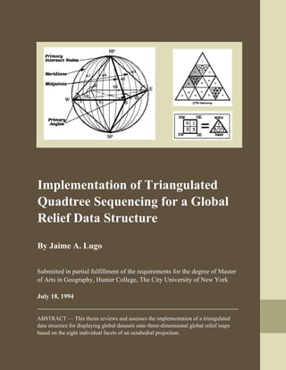
  • 51. CHAPTER6 Future Applications of the Triangulated Quadtree Structure 6.1: Conditions and Data Reg,uirements The elevation dataset, ETOP05 is available on CD-ROM from the National Geophysical Data Center, NOAA; a full description is found in Appendix C: ETOP05 Documentation. After geographically referencing the ETOP05 dataset to a set of latitude/ longitude coordinates, it may be used to locate each node on the tessellation structure. Note that, since elevation data are irregularly spread, they will produce irregularly shaped triangle facets. This problem calls for more complex algorithms than if the nodes were fitted to the surface of a perfect sphere. A perfect sphere is used because it permits the application of a simple isohedral tesse3llation, such as the one already developed by Dutton (1984). To optimize the model's data structure, the elevation data was stored on the TQS structure - using a quaternary tessellation similar to the QTM structure. A quadtree structure is again recommended because it is a hierarchical database that fits the requirements for a global data structure (Tobler and Chen, 1986). The next question is then how to retrieve elevation data from a raster-based quadtree structure and reference it to each node on the vector-oriented triangular tessellation. This can be solved either with Morton Sequencing (Cebrian et. al., 1985; Lauzon et al., 1985; Burrough, 1986), or with the Triangulated Quadtree Structure (TQS). Each quadrant level on the quadtree is given a binary digit based on the quadtree level and its relative location along the coordinate plane. Morton Sequencing then allows the computer to read the actual quadtree's location directly from the binary string. 43
  • 52. 6.2: The Application Process The application process that portrays the finalized data structure onto a three- dimensional graphical interface - called a Three-Dimensional Planetary Relief Model - is now introduced. The first step is to fit an isolateral octahedron inside a perfect sphere (Figure 6.1). The points where the octahedron touches the sphere along its great circles are called the Primary Intersect Nodes, or PINs, for short. These PINs will then constitute the octahedron's six (6) cardinal points in Fig. 18 (N, E, S, W, NP, SP). These PINs correspond to the o0 , 90°, 180°, 90°W meridians, the north pole (NP) and the south pole (SP) (Laurini and Thompson, 1992, pp. 246-7, Figure 6.22). SP Figure 6.1: Primary Intersect Nodes (PINs), Midpoints, and Primary Angles. , • •.,;,,.~ X, ~ , .-. ,.?. ,•,:.-.-X•?. ... ' • , X ?.',,:-• 44
  • 53. Once all pins are connected to the nodes representing the poles (NP, SP), the first level of the octahedral sphere is complete. To reduce storage and search procedures, each node will be automatically georeferenced to the elevation database. It is thus possible to use a Triangulated Irregular Network (TIN) to visualize the octahedral nodes, especially since a tessellated triangle inherently contains topologically oriented data (Dutton, 1988). The steps involved below will produce each successive tessellation level: 1. Split all arcs at their midpoints. 2. Place a georeferenced node at each ofthe new midpoints. 3. Elevate (or lower) the midpoint nodesfrom the octahedron's center, based on the corresponding elevationfor each node. 4. The arcs and nodes belonging to polygon areas oflow reliefare left intact. Areas with high relief will be tagged as further subdivision areas. Low and high relief values are computed using statistical elevation variance (spread ofpoints awayfrom the mean). 5. Save all P/Ns and newly elevated nodes under a new tessellation level. 6. Repeat process until desired tessellation level is achieved. This procedure, once completed, will be capable of tessellating the octahedron to almost any level of tessellation, up to the resolution of the dataset. Once the source code has been developed, tested and implemented, output becomes the next problem to overcome. Hardware will limit the output's quality to an n-dimensional virtual projection on the monitor. The model will need further modification to display only those areas directly facing the user. This may be solved by fitting the octahedral skeleton into a TIN structure, and transform it using any of various "watershed analysis" algorithms. In addition, the user must be able to select those areas he/she wishes to display. Since the dataset is georeferenced using individual quadrants, the user may select any area of the globe, provided that it all belongs within a specific quadrant at the corresponding tessellation level. The user delimits the map extent based on the east and west coordinates 45
  • 54. of the desired octant, along with a choice between the northern and southern hemispheres. These corners will be the map's ground control points. For final display, the desired area may eventually be transformed from a three- dimensional structure to either 1) a two-dimensional digital elevation model (DEM), or 2) a one-dimensional map projection. For a two-dimensional DEM, Cebrian et. al.,(1985) proposed that "digital elevation models be integrated into the linear quadtree GIS by using Morton numbers as addresses for cell elevation data in a one-dimensional array or file," (Cebrian, 1985, p. 58). These dimensional transformations may serve as both the display methods and testing tools for determining the accuracy of the model. On the other hand, to produce a one-dimensional map projection, the ground control points may be used to statistically transform the three-dimensional model to a one- dimensional map. This statistical method is known as rubber sheeting (Clarke, 1990, p. 147). Although this technique adds a large degree oferror by stretching the map extent into a flat surface, it produces aesthetically pleasing maps for any part of the world at a scale limited only by the tessellation levels and resolution of the data. The dataset must also be large enough for a true global approximation, although it may still be tessellated to any resolution desired. If the dataset is too small, it is then recommended that the data analysis be performed on individual octants. 6.3: Future Applications Future applications involve substituting the global relief dataset with other types of ordinal data, such as population density, crime distribution, income, spread of disease, temperature, and so forth. If the desired dataset is not sequentially ordered, it must be modified and fitted to the planetary model, such that it can be hierarchically stored. 46
  • 55. CHAPTER 7 Conclusion, Summary & Importance In conclusion, the Triangulated Quadtree Structure addressing algorithm successfully linked the land portion of the ETOP05 dataset to the Interrupted Collignon Equal Area Projection. Therefore, the proposed planetary relief geographic information system is now a feasible model for the application global spatial data. A 2.5-dimensional elevation model was developed using a triangular tessellation to achieve any resolution desired, the first step on developing an isohedral quadtree structure for the storage of elevation data was presented, and a set of grid points were georeferenced into a triangular coordinate grid. Each chapter reviewed the application of square- triangle-based grids, algorithms, triangular tessellations, and quadtrees. The accuracy and precision of the TQS addressing numbers increased with every tessellation, until each address represented each elevation point up to the resolution of the original dataset. Once the georeferenced data is stored in the triangulated quadtree structure, areas with little reliefwill be left intact, while areas with high relief are further subdivided to provide higher resolutions in those areas. The result has been a model that fitted the Earth's surface onto the surface of a map projection that is easily transformed into a paper octahedron. This accomplishment will eventually lead to a three-dimensional model capable of providing a three-dimensional image of the globe, two-dimensional digital elevation models of medium- to small scale areas, or one- dimensional map projections given the desired level of tessellation, map scale and a coordinate range. Furthermore, the Earth's elevation was the original data type proposed (and used) to define the surface ofthe geodesic octahedron, it is not the only attribute applicable to this model. Other attributes may be statistically fitted to the planetary model include population density, income, meteorological data, incidence of a particular disease, and others. In other 47
  • 56. words, this model could be viewed as a three-dimensional choropleth map for the entire world. Other global datasets include biodiversity distribution and soil types (Csillag, 1994). On the other hand, while this method offers simplicity and geolocational precision, it lacks the ability to measure scale throughout the octahedron's surface. As the levels of tessellation change, so does the length of every triangular segment, meaning that scale continues to change throughout the globe's surface and becomes impossible to measure (Dutton, 1989b). In other words, while a coordinate may tell the user where an object is, it fails to inform the actual size of this object. Thus, despite this weakness in scale measurement, the recent acquisition of the necessary technology to achieve the stated goals makes the proposed application likely to be ready in the near future. Since squares began their incursion and conquest of the cartographic world, people have taken for granted that a coordinate system must be a discrete, rather than continuous, set of points. Therefore, most spherical projections are subjected to inaccuracies and precision problems developing from trying to fit a circle into a square. This is precisely the type of error that the proposed global relief geographic information systems was designed to address. 48
  • 57. REFERENCES Abel, D. J. (1984). "A B+-Tree Structure for Large Quadtrees." Computer Vision, Graphics and Image Processing, v. 27, pp. 1-18. Burrough, P. A. (1986). Principles of Geo~hical Information Systems For Land Resources Assessment. New York: Clarendon Press. Cebrian, Juan A. James E. Mower, and David M. Mark (1985). "Analysis and Display of Digital Elevation Models Within a Quadtree-Based Geographic Information System." Proceedings Auto-Carto 7, Falls Church, VA: ASPRS/ACSM, pp. 55-64. Chen, Zi-Tan and Donna Peuquet (1985). "Quadtree Spatial Spectra Guide: A Fast Spatial Heuristic Search in a Large GIS." Proceedings Auto-Carto 7, Falls Church, VA: ASPRS/ACSM. Clarke, K. C. (1990) Analytical and Computer Cartography. New Jersey: Prentice Hall, pp. 15, 147. Clarke, K. C. (1994). Interview. New .York: Department of Geology and Geography, Hunter College of the City University of New York. Csillag, Ferenc (1993). "Variations and Hierarchies: Toward Linking and Integrating Structures." NCGIA: 2nd International Conference/Workshop on Integrating Geographic Information Syst~ins and Environmental Modeling. Breckenridge, Colorado, September 1993. Dutton, Geoffrey. (1984). "Geodesic Modelling of Planetary Relief." Cartographica, v21, Numbers. 2 & 3, pp. 188-207. Dutton, Geoffrey (1988). "Modeling Locational Uncertainty via Hierarchical Tessellation." ed. Goodchild Michael and Sucharita Gopal. Accuracy of Spatial Databases. New York: Taylor & Francis, pp. 123-140. Dutton, Geoffrey (1989a). "Computational Aspects of Quaternary Triangular Meshes." Prime Park, MS: Prime Computer, Inc. (unpublished). Dutton, Geoffrey (1989b). "The Fallacy of Coordinates." Prime Park, MS: Prime Computer, Inc. (unpublished). Dutton, Geoffrey (1989c). "Glossary. of Basic, Obscure and Invented Geonomic Terms."Prime Park, MS: Prime Computer, Inc. (unpublished). Dutton, Geoffrey (1989d). "Zenithial Orthotriangular Projection." Spatial Effects. Prime Park, MS: Prime Computer, Inc. (unpublished). 49
  • 58. Dutton, Geoffrey (1991). "Improving Spatial Analysis in GIS Environments." Proceedings Auto-Carta 10, 1991, pp. 168-185. Goodchild, Michael (1988). "The Issue Of Accuracy In Spatial Databases." Building Databasesfor Global Science, Mounsey, H., and Tomlinson, R. (editors). London: Taylor & Francis, pp. 31-48. Hedley, Justin (1992). "3-D Migration via McClellan Transformations on Hexagonal Grids." Geophysics, v57, no. 8, pp. 1048-1053. Ibbs, T. J. and A. Stevens (1987). "Quadtree Storage of Vector Data." Presented at GIS- LP'87, Lisbon, September 14-18. Klette, Reinhard (1985). "The m-Dimensional Grid Point Space;'' Computer Vision, Graphics and Image Processing, v30, pp. 1-12. Koffman, Elliot B. and Frank L. Friedman (1990). Problem Solvini and Strnctured Proifammini in FORTRAN 77. New York: Addison-Wesley Publishing Company, Inc. Laurini R. and D. Thompson (1992). Fundamentals of Spatial Information Systems. New York: Academic Press Ltd. Lauzon, J., D. Mark, L. Kikuchi, and A. Guevara (1985). "Two-Dimensional Run- Encoding for Quadtree Representation." Computer Vision, Graphics and Image Processing, v30, pp. 56-69. Lillesand and Kieffer (1987). Remote Sensini and Imaie Interpretation. New York: John Wiley & Sons. Mark, David M. and Jean Paul Lauzon (1985). "Approaches for Quadtree-based Geographic Informati9n Systems at Continental and Global S9ales." Proceedings Auto-Carto 7, Falls Church, VA: ASPRS/ACSM, pp. 355- 364. The Towson State University Manual of GIS (1990). Department of Geography, Towson State University, pp. 1-13. Martin, Johannes (1982). "Organization of Geographical Data with Quad Trees and Least Squares Approximation." Proceedings, IEEE Computer Society Conference on Pattern Recognition and Image Processing. Las Vegas, Nevada. Morton, G. M. (1966). "A Computer Oriented Geodetic Data Base, and a New Technique in File Sequencing." IBM Canada Ltd. Peucker, T. K. Fowler, R. J., Little, J.J., and Mark, D. M. (1986). Digital Representation of Three-djmensjonal Surfaces by Trianiulated Irre~ular Networks (TIN). Technical Report Number 10, United States Office of Navel Research, Geography Programs. 50
  • 59. Peucker, Thomas K., et al (1978). "The Triangulated Irregular Network." Proceedings of the Digital Terrain Models Symposium of the American Society for Photogrammetry!American Congress on Surveying and Mapping. St. Louis, Missouri, USA, pp. 516-540. Peuquet, D. J. (1984). "A Conceptual Framework and Comparison of Spatial Data Models." Cartographica 21, 4(1984), 66-113. Peuquet, Donna J. ·and Duane F. Marble (1990). Introductory Readings in Geographic Infonnation Systems. New York: Taylor & Francis. Pham, S. (1986). "On the boundary of Digital Straight Line Segments." Proceedings, Computer Graphics, Tokyo, 1986, in Advanced Computer Graphics (T. L. Kunni, Ed.), pp. 79-109, Springer-Verlag, Tokyo. Pham, S. (1987). "Equations of digital straight lines," in Proceedings Computer Graphics, Tokyo, 1987 (T. L. Kunni, Ed.), pp. 221-248, Springer-Verlag, Tokyo. Rogers, C. A. (1984). Packin~ and Coverin~. Boston: Cambridge University Press. Rosenfeld, A. (1974). "Digital Straight Line Segments." IEEE Transactions, Computing, C-23, pp. 1264-1269. Samet, Hanan (1990a). Design and Analysis of Spatial Data Structures. New York: Addison-Wesley Publishing Company. Samet, Hanan (1990b). Applications of Spatial Data Strnctures. New York: Addison- Wesley Publishing Company. Samet, Hanan and Robert Webber (1985). "Storing a Collection of Polygons Using Quadtrees." ACM Transactions on Graphics, Vol. 4, pp. 182-222. Snyder, J. P. and P. M. Voxland (1989). An Album of Map Projections. Reston, VA: Department of the Interior, U.S. Geological Survey, Denver, CO. Tobler, Waldo and Zi-tan Chen (1986). "A Quadtree for Global Information Storage." Geographical Analysis, v18(4), pp. 360-371. Tsai, Victor J. D. and Alan p. Vonderohe (1993). "Delaunay Tetrahedral Data Modelling For 3-D GIS Applications." Proceedings, GIS!LIS'93, Minneapolis, MN. Walker, Susan S. "An Introduction to Geographic Information System Terminology." Hunter College, Department ofGeology and Geography, GEOG 790, Independent Research Project, December 22, 1987. 51
  • 60. Wu, Li-De (1982). "On the Chain Code of a Line." IEEE Trans. Pattern Analysis, Machine Intelligence. PAMI-4(3), pp. 347-353. Wuthrich C. A., and P. Stucki (1991). "An Algorithmic Comparison Between Square- and Hexagonal-Based Grids." Computer Vision, Graphics and Image Processing: Graphical Models and Image Processing. v53(4), pp. 324-339. 52
  • 61. APPENDIX A: C Source Code The following is a listing of the enclosed C source code files. Each file contains a description header, which provides a briefintroduction to each file, author(s), and functions call~d. Each file was printed in a special format, which prints two file pages into one page. File Name No, of Pa~es 1. Collignon.c 2 2. Main.c 1 3. Get_TQS.c 3 4. Write_Etopo5.c 2 5. Swap.c 1 53
  • 62. I* ************************************************************ *I /* Collignon.c REVISED TO DEAL WITH ONE OCTANT AND SCALED */ /* Function to transform a point to the Collignon Projection. •; /* The Collignon Projection is a pseudocylindrical, equal-area •; /* projection. Meridians are equally spaced straight lines •; /* converging at the North Pole, while parallels are unequally */ /* spaced straight lines, farthers apart near the North Pole, •; ;• closest near the South Pole, and perpendicular to the •; /* central meridian. Scale is true along latitudes 15deg5l'N. •; I* ************************************************************ */ finclude •extern.h" tinclude <math.h> #define PI 3.141592654 #define R 6378137 tdefine S 0.00000005 POINT /* Radius of the Earth */ /*scale= 1:50,000,000 */ collignon(Point) O; POINT Point; double sqrt_of_pi, two_pi_over_360, r_times_s, temp, lambda_sub double mod_x, mod__y, rotate, Scos30, Ssin30; int i; float before x; POINT project; two_pi over 360 =PI/ 180.0; sqrt_of_pi ~ pow(PI, 0.5); r_times_s = (double) R * s; Scos30 = xrange • 0.866025403; Ssin30 = xrange * 0.5; /* Assign the octant*/ if (Point.octant== 0) else l Point.octant= 2; if (Point.y > 0.0) l Point.octant= 4; I else~ if (Point.x < 90.) Point.octant= 3; if (Point.x < O.) Point.octant= 2; if (Point.x < -90.) Point.octant= 1; Point.octant= 5; if (Point.x < 90.) Point.octant= 8; if (Point.x < 0.) • Point.octant= 7; if (Point.x < -90.) Point.octant= 6; switch (Point.octant) case 1: central meridian -135; case 2: case 3: case 4: case 5: case 6: case 7: case B: lat lo= 0.0; lat-hi= 90.0; long lo= -180.0; long-hi= -90.0; break; central meridian= -45; lat lo~ 0.0; lat-hi= 90.0; long lo= -90.0; long-hi= 0.0; break; central meridian= 45; lat lo~ 0.0; lat-hi= 90.0; long lo= 0.0; long-hi= 90.0; break; central meridian= 135; lat lo~ o.o; lat-hi= 90.0; long lo= 90.0; long-hi= 180.0; break; central meridian= 135; lat lo ~ -90.0; lat-hi= 0.0; long lo= 90.0; long-hi = 180. O; break; central meridian= -135; lat lo~ -90.0; lat-hi= 0.0; long lo= -180.0; long-hi= -90.0; break; central meridian= -45; lat lo~ -90.0; lat-hi= 0.0; long lo= -90.0; long-hi= 0.0; break; central meridian= 45; lat lo~ -90.0; lat-hi= 0.0; long lo= 0.0; long-hi= 90.0; break; /* Deal with the rotation of the central meridian*/ lambda_sub_O = two_pi over_360 * central_meridian; if ((Point.x - centraI meridian) > 180.0) Point.x -= 360:o; else if ((Point.x - central_meridian) <= -180.0)
  • 63. f_p1; temp); Point.x += 360.0; /* Convert to radians*/ project.x = Point.x • two_pi_over_360; project.y = Point.y * two_pi_over_360; project.octant= Point.octant; project.elev= Point.elev; 1• * For southern hemisphere invert •1 if (Point.octant> 4) I project.y *= -1.0; I /• Collignon transformations•/ temp= pow((l.O - sin((double) project.y)), 0.5); project.x = 2.0 * r_times_s * (project.x - lambda_sub_O) •temp/ sqrt_o project.y = cos(30. * two_pi_over_360) * sqrt_of_pi * r_times_s * (1.0 - 1• • For southern hemisphere, reflect about axis of central meridian •1 if (Point.octant> 4) I project.x •= -1.0; I return (project);
  • 64. ,.....•...•...•....•..•..••....•.......•....•.., /* Main.c: */ /* - Read the ETOP05 dataset from its */ /* file into a structure. */ I* - Author: Keith C. Clarke */ I* - Last edited on 7-12-94. */ /******************************•***************/ tinclude <math.h> tinclude <stdio.h> linclude •extern.h" ldefine INPOT FILE "/home/popocatepetl/kclarke/world/etopo5/world.lan• main() - l void POINT FILE read erdas(); Point, collignon(); *fp; fp = fopen(INPOT_FILE, "r"); (void) read erdas(fp); (void) fclose(fp);
  • 65. /************************************************/ /* Get TQS.c: /* - - Author: Jaime Lugo /* - Last modified 07-12-94 /* - Contains functions: /* 1. Get TQS () I* 2. Tessellate 0 *I */ */ */ *I *I /************************************************/ #include <stdio.h> tinclude <math.h> tinclude <ctype.h> linclude "header.h" tinclude •extern.h" tdefine FALSE 0 tdefine TRUE 1 1·····················································1/* FUNCTION Get TQS(): */ /* - Calcuiates xrange, yrange for all octants. */ /* - Calls Function Tessellate(), which gets */ /* the TQS address for the erdas (x,y) point. */ /*****************************************************/ POINT Get TQS (Point) - POINT Point; POINT int int double collignon(), Setup; tqs; Tessellate(); xrange, yrange; /* get x-range value for whole octant*/ setup.x = -90.0; setup.y = o.o; Setup.octant= O; Setup = collignon(Setup); xrange = Setup.x; if (xrange < 0.0) xrange *= -1.0; xrange *= 2.0; /* Original xrange = 0.565248 */ /* get y-range value for whole octant*/ Setup.x = -45.0; Setup.y = 90.0; Setup.octant = .O; Setup= collignon(Setup); yrange = Setup.y; /* Original yrange = 0.489519 */ /* printf("n Original xrange = f", xrange); */ /* printf("n Original yrange = fnn•, yrange); */ /* Transform Point.x and Point.y Point = collignon(Point); /* printf("x,y After Collignon: /* printf("gets placed in octant into a Collignon coordinate. */ (f f) •, Point.x,Point.y); */ dnn", Point.octant); */ /* Get the QTM address for that point. */ Point.qtm = Tessellate(Point, xrange, yrange); /* printf("Tessellate() returns [X] in Hex notation.nn",tqs); */ return (Point); I /******************************************************/ /* FUNCTION Tessellate(): */ I* - Ftn tessellates each triangular octant up */ /* to the maximum depth specified. */ /* - MAXDEPTH has been assigned 12 recursions. */ I* - Finally, ftn returns a variable address */ /* up to 24-bits long (3 bytes) */ /******************************************************/ int Tessellate(Point, POINT xrange, yrange) Point; double xrange, yrange; POINT int short double Testyt; depth, new qtm, qtm~ MAXOEPTH end loop, do shift; before x, midpt y, cos 180, sin-180, cos-240, sin-240; Test_J>t = Point; - cos 240 = 0.9973288; sin-240 = 0.0730431; cos-180 = 0.9984972; sin-180 = 0.0548037; qtm- = 00; new qtm = 00; do shift = TRUE; midpt_y = (0.5 • yrange); 12; /* Temp storage for (x,y) */ /* counts depth level */ /* stores qtm triangle number*/ /* stores shifted QTM address*/ /* Maximum depth*/ /*flag*/ /*flag*/ /* midpoint of y-axis*/ I* cos 180 = cos(PI) /* sin-180 = sin(PI) /* stores the final qtm address in hex /* stores qtm address just assigned /* bit-shift if "do shift• is true /*****************************************************/ /* TESSELLATION LOOP: Body of function Tessellate() */ /* Tessellate only to the max depth for the dataset: */ 1·····················································1for (depth= O; depth< MAXDEPTH; depth++) { end loop= FALSE; /* -Check whether MAXOEPTH has been reached. */ if (depth== (MAXDEPTH - 1)) do shift= FALSE; /**********************************************/ /* if point falls in qtm triangle one= qtm.1 */ /**********************************************/ if ((Test_pt.y > midpt_y) && (Test_J>t.y <= yrange)) { /* Assign point to triangle #1 and shift left */ /* while the tessellation hasn't reached MAXDEPTH. */ new qtm = 1; /* printf("Ol "); */ qtm = (new_qtm I qtm); /*bit-parser*/ /* ... OR ... */ *I *I */ *I *I