fast fractal image compression

1. fractal and fractional
Article
Image Compression Using Fractal Functions
Olga Svynchuk 1 , Oleg Barabash 1, Joanna Nikodem 2, Roman Kochan 2 and Oleksandr Laptiev 3,*
Citation: Svynchuk, O.; Barabash, O.;
Nikodem, J.; Kochan, R.; Laptiev, O.
Image Compression Using Fractal
Functions. Fractal Fract. 2021, 5, 31.
https://doi.org/10.3390/
fractalfract5020031
Academic Editors: Carlo Cattani,
Svitlana Kuznichenko and
Mikolaj Karpinski
Received: 15 February 2021
Accepted: 9 April 2021
Published: 14 April 2021
Publisher’s Note: MDPI stays neutral
with regard to jurisdictional claims in
published maps and institutional affil-
iations.
Copyright: © 2021 by the authors.
Licensee MDPI, Basel, Switzerland.
This article is an open access article
distributed under the terms and
conditions of the Creative Commons
Attribution (CC BY) license (https://
creativecommons.org/licenses/by/
4.0/).
1 Department of Automation of Heat and Power Engineering Processes, National Technical University of
Ukraine “Igor Sikorsky Kyiv Polytechnic Institute”, 37 Peremohy Ave., 03056 Kyiv, Ukraine;
7011990@ukr.net (O.S.); bar64@ukr.net (O.B.)
2 Department of Computer Science and Automatics, University of Bielsko-Biala, 2 Willowa Str.,
43-309 Bielsko-Biala, Poland; jnikodem@ath.bielsko.pl (J.N.); rkochan@ath.bielsko.pl (R.K.)
3 Department of Information and Cybersecurity Systems, State University of Telecommunications,
7 Solomenska Str., 03110 Kyiv, Ukraine
* Correspondence: alaptev64@ukr.net; Tel.: +380-674348001
Abstract: The rapid growth of geographic information technologies in the field of processing and
analysis of spatial data has led to a significant increase in the role of geographic information systems
in various fields of human activity. However, solving complex problems requires the use of large
amounts of spatial data, efficient storage of data on on-board recording media and their transmission
via communication channels. This leads to the need to create new effective methods of compression
and data transmission of remote sensing of the Earth. The possibility of using fractal functions for
image processing, which were transmitted via the satellite radio channel of a spacecraft, is considered.
The information obtained by such a system is presented in the form of aerospace images that need
to be processed and analyzed in order to obtain information about the objects that are displayed.
An algorithm for constructing image encoding–decoding using a class of continuous functions that
depend on a finite set of parameters and have fractal properties is investigated. The mathematical
model used in fractal image compression is called a system of iterative functions. The encoding
process is time consuming because it performs a large number of transformations and mathematical
calculations. However, due to this, a high degree of image compression is achieved. This class of
functions has an interesting property—knowing the initial sets of numbers, we can easily calculate
the value of the function, but when the values of the function are known, it is very difficult to return
the initial set of values, because there are a huge number of such combinations. Therefore, in order to
de-encode the image, it is necessary to know fractal codes that will help to restore the raster image.
Keywords: fractal; fractal function; fractal properties; self-similarity; fractal compression; iterated
function system; affine transformations
1. Introduction
Remote sensing of the Earth (REE) is the observation of our planet and the determina-
tion of the properties of objects on the earth’s surface, obtained with the help of imaging
devices installed on aircraft and artificial satellites of the Earth (Figure 1). The obtained
data are aerospace images of the observed part of the earth’s surface in digital form in the
form of raster images (Figures 2 and 3). These data are subject to further detailed analysis,
namely, the determination of quantitative characteristics of the object under study, which
are necessary to predict the development of a phenomenon or process. The processing and
interpretation of remote sensing data is closely related to digital image processing. Remote
sensing allows one to obtain from space high-quality images of the earth’s surface, which
help to solve practical problems in various fields of human activity. However, the amount
of this graphical information is very large and needs to be compressed when transmitting
data over communication channels and then used in geographic information systems.
Today, fractal methods are often used to transfer images from satellites to the ground,
which help to give a better picture. The main feature of these methods is the property of
Fractal Fract. 2021, 5, 31. https://doi.org/10.3390/fractalfract5020031 https://www.mdpi.com/journal/fractalfract

2. Fractal Fract. 2021, 5, 31 2 of 14
self-similarity of the image. Such methods provide large compression ratios. However, they
need significant development while taking into account many criteria (speed, compression
ratio, quality during decompression). They can be considered a real alternative to JPEG for
many classes of images used in everyday life.
Figure 1. Remote sensing of the Earth.
Figure 2. Fires on the planet Earth, 2020.
Fractal image compression (fractal transformation, fractal encoding) is a lossy image
compression algorithm based on the iterated function system to images [1,2]. The encoding
algorithm is encoded [3]. The concept of the fractal method was first introduced in 1990
by the British mathematician Michael Barnsley [4]. It consists of the fact that in the image
it is necessary to find separate self-similar fragments which are repeated many times. He
proved a class of theorems that allowed for the effective compression of images. In [5],
Arno Jacquin described a new method of fractal encoding, in which the image is divided
into domain and rank blocks, which cover the entire image. This approach became the
basis for the creation of new fractal encoding methods used today. Jacquin’s method was
perfected by Yuval Fisher [6] and other scientists.

3. Fractal Fract. 2021, 5, 31 3 of 14
Figure 3. Hurricane Laura, USA, 2020.
A large number of scientific papers are devoted to the study of the effectiveness of
the fractal image compression method [7–22]. For example, in [7] the algorithm of fractal
compression of images using space-sensitive hashing is considered. Various methods
are proposed in [8–13] aimed at reducing the volume of domain blocks, which makes it
possible to reduce the encoding time of the search. In [8], a discrete cosine transform was
used to classify all domain blocks into a number of classes, in [9] R-trees were used for this
purpose, and in [10] a self-organized neural network was used. In [11,12], scientists use a
genetic algorithm to search for optimal domains. In [13], the search is limited by the degree
of information entropy of the domains. In [14–22], the variants of optimization and increase
in fractal encoding speed and possibilities of their practical application are analyzed.
Today, the topic of fractal compression algorithms is still being actively studied.
The aim of our research is to model the class of fractal functions, study their properties
and establish the possibility of their application for an efficient algorithm for encoding
images that are presented in digital form.
2. Materials and Methods
Fractal encoding is a mathematical process for encoding rasters into a set of mathe-
matical data that reproduces the fractal properties of a given image. This encoding is based
on the fact that all natural objects have a lot of similar information in the form of repetitive
patterns. They are called fractals. Fractal decoding is a reverse process in which a system
of fractal codes is converted into a raster [14].
The concept of fractal was proposed by the French-American mathematician Benoit
Mandelbrot. In 1977, he published “Fractal Geometry of Nature”, describing repeti-
tive drawings from everyday life [23]. According to him, many geometric figures con-
sist of smaller figures, which when being enlarged repeat accurately a larger figure
(Figures 4 and 5). After conducting research, he also found that fractals have chaotic
behavior, a fractional infinite dimension (how completely a fractal fills a space when magni-
fied to smaller details), and can be described mathematically using simple algorithms [24].
It is known that many geographical objects have fractal properties—contours of coasts
and oceans, rivers, mountain gorges, and state borders where they are drawn by natural
contours [24].

4. Fractal Fract. 2021, 5, 31 4 of 14
Figure 4. Koch snowflake.
Figure 5. Sierpinski’s triangle.
For the constructive task of such fractal objects and their analytical research today
in mathematics, various systems of representation and the encoding of real numbers are
widely applied: with the finite and infinite, constant and variable alphabet, with natural
and the whole negative, rational and irrational bases, etc. These are s-s and non-s-s, Q-
representations, chain fractions, real numbers in the series Cantor, Lurot, Engel, Sylvester,
Ostrogradsky–Sierpinski–Pierce, etc [25–28]. The creation of a new encoding system for
the fractional part of a real number significantly expands the range of such objects, which
are relatively simply formally described and studied.
In our work, we use an encoding system with a finite alphabet to build a new math-
ematical model that will be used in fractal image compression. The model is based on a
continuous class of continuous functions that depend on a finite set of parameters and
have fractal properties.
Let A5 = {0, 1, 2, 3, 4} be the alphabet of the five-digit numeral system, L ≡ A5 ×
A5 × A5 × . . . A5 × . . . be a space of the sequences of elements of the alphabet and let
Q∗
5 = qij
, i ∈ A5, j ∈ N be an infinite stochastic matrix with positive elements qij 0
and the following properties:
Q∗
5 = qij
=






q01 q02 . . . q0j . . .
q11 q12 . . . q1j . . .
q21 q22 . . . q2j . . .
q31 q32 . . . q3j . . .
q41 q42 . . . q4j . . .






,
1. q0j + q1j + q2j + q3j + q4j = 1, ∀j ∈ N (stochasticity);
2.
∞
∏
j=1
max
q0j, q1j, q2j, q3j, q4j = 0 (continuity).

5. Fractal Fract. 2021, 5, 31 5 of 14
The known theorem [25] states that for any x ∈ [0; 1] there exists a sequence (αk) ∈ L
such that
x = βα11 +
∞
∑
k=2
βαkk
k−1
∏
j=1
qαj j
!
= ∆
Q∗
5
α1α2...αk..., (1)
where β0j = 0, βij ≡ q0j + q1j + . . . + qi−1,j = βi−1,j + qi−1,j, i ∈ {1, 2, 3, 4}, j ∈ N.
The representation of the number x in the form of series (1) is called Q∗
5-expansion
while the symbolic notation x = ∆
Q∗
5
α1α2...αk... is called Q∗
5-representation, and a number
αk = αk(x) is called j-th digit in the representation of x.
If all the columns of the matrix qij
are identical, i.e., qij = qi for any j ∈ N, then
Q∗
5-representation is called Q5-representation. If qi = 1
5 is for all i ∈ A5, then the Q5-
representation is a classic a five-digit representation.
Each irrational number has a unique representation, but some rational numbers
have two representations. These are numbers with the representations ∆
Q∗
5
α1α2...αm(0)
=
∆
Q∗
5
α1α2...αm−1[αm−1](4)
. By agreement, we use only one of two representations of a rational
number containing period (0). Then, we have the uniqueness of the Q∗
5-representation of a
number.
The concepts of cylinder and Hausdorff–Besicovitch dimension are important for
image geometry. We will revisit them [25].
Definition 1. A set of all numbers x ∈ [0; 1] that have Q∗
5-images with the first digits of
c1, c2, . . . , cm, respectively, is called a cylinder of rank m ∆
Q∗
5
s1s2...sm with base c1, c2, . . . , cm.
The cylinders have the following properties:
(1) Cylinders of rank m are a union of cylinders of rank m + 1, i.e.,
∆
Q∗
5
c1c2...cm = ∆
Q∗
5
c1c2...cm(0)
∪ ∆
Q∗
5
c1c2...cm(1)
∪ ∆
Q∗
5
c1c2...cm(2)
∪ ∆
Q∗
5
c1c2...cm(3)
∪ ∆
Q∗
5
c1c2...cm(4)
;
(2) A cylinder ∆
Q∗
5
s1s2...sm is a segment with the endpoints
a = ∆
Q∗
5
s1s2...sm(0)
= βc11 +
m
∑
k=2
βckk
k−1
∏
j=1
qcj j
!
, b = ∆
Q∗
5
s1s2...sm(4)
= a +
m
∏
i=1
qcii;
(3) Basic metric ratio:
∆
Q∗
5
s1s2...sm(i)
∆
Q∗
5
s1s2...sm
= qi,m+1 = const;
(4) max∆
Q∗
5
s1s2...smi = min∆
Q∗
5
s1s2...sm[i+1]
, i = 0, 1, 2, 3;
(5) For any sequence (cn) ∈ L, the equation holds:
∞
∩
m=1
∆
Q∗
5
s1s2...sm = ∆
Q∗
5
s1s2...sm... ≡ x ∈ [0; 1].
Let (M, ρ) be a metric space, E a bounded subset of M and d(E) denote the diameter
of the set E. Let ΦM be a family of subsets of the space M such that for an arbitrary set
E ⊂ M and, for each number ε 0, there exists an at most countable ε-covering {Ej} of E
Ej ∈ ΦM, d Ej
≤ ε
. Let α be a positive number.

6. Fractal Fract. 2021, 5, 31 6 of 14
Definition 2. The α-dimensional Hausdorff measure of a bounded set E of a metric space (M, ρ) is
defined by
Hα(E) = lim
ε→0
inf
d(Ej)≤ε
(
∑
j
dα
Ej
)#
= lim
ε→0
mα
ε (E),
where the infimum is taken over all at most countable ε -coverings
Ej of E, Ej ∈ ΦM.
Definition 3. The positive number
α0(E) = sup{α : Hα(E) = ∞} = inf{α : Hα(E) = 0}
is called the Hausdorff–Besicovitch dimension of the set E.
Using Q∗
5-representation of numbers, denote the function by the equality:
f (x) = γα1(x)1 + γα2(x)2gα1(x)1 + γα3(x)3gα2(x)2gα1(x)1 + . . . =
= γα1(x)1 +
∞
∑
k=2
γαk(x)k
k−1
∏
j=1
gαj(x)j
!
≡ ∆
G∗
5
α1(x)α2(x)...αk(x)...
(2)
where (gn) = (g0n, g1n, g2n, g3n, g4n), n ∈ N is a sequence of vectors such that:
g0n = εn+2
4 , g1n = −εn
4 , g2n = 0, g3n = −εn
4 , g4n = εn+2
4 ,
γ0n = 0, γ1n = εn+2
4 , γ2n = 1
2 = γ3n, γ4n = 2−εn
4 ,
where γi+1,n = γin + gin, i ∈ N,
(3)
(εn) is a sequence of positive real numbers with 0 ≤ εn ≤ 1.
Function properties [29]:
(1) The function is continuous on [0; 1] and acquires all its values from [0; 1];
(2) The function has no intervals of monotonicity, except for intervals of constancy, if
εn 6= 0 is satisfied for an infinite set of values of n;
(3) is a function of limited variation if
∞
∑
k=1
εk ∞;
(4) is a singular Cantor-type function with a Hausdorff–Besicovitch fractal dimension
log5 4;
(5) the graph of the function is symmetric about point
1
2 ; 1
2
.
3. Results
We describe the method of fractal encoding of images using this class of nonmonotonic
singular functions. The image is placed in a single square. We define two vectors Q and G
such that:
Q =
q0j, q1j, q2j, q3j, q4j , qij 0, q0j + q1j + q2j + q3j + q4j = 1, , j ∈ N,
G = {g0k, g1k, g2k, g3k, g4k}, gik 0, g0k + g1k + g2k + g3k + g4k = 1, k ∈ N.
The first vector divides our image along the abscissa axis into five Q-cylinders (rank
areas) that do not intersect (Figure 6), the length of q0j, q1j, q2j, q3j, q4j respectively. The
second vector on the y-axis specifies a set of G-cylinders that can overlap (Figure 7), the
length of g0k, g1k, g2k, q3k, q4k each, respectively.

7. Fractal Fract. 2021, 5, 31 7 of 14
Figure 6. Q-cylinders of the 1st and 2nd rank.
Figure 7. G-cylinders of the 1st and 2nd rank.
We take two identical images of 1 × 1 size. The first image is divided into Q-cylinders,
and the second image is divided into G-cylinders (they describe similar parts and are used
in constructed decoded images). For each method of search of Q-cylinders, the nearest G-
cylinder for which the distributed features can be approximated by the distribution of a rank
area is selected. For the best approach to the G-cylinders, use the official conversion, which
helps to change the brightness and contrast. If the desired approximation is not achieved,
each cylinder of the rank area again extends to the appearance of the corresponding parts
and the process is repeated. The numbers of the Q- and G-cylinders that were used in the
encoding process and helped to obtain the desired results, together with the coefficients of
affine transformations, are written to the file. These results will then be used in decoding.
Therefore, in the original image there is a search for self-similar areas, which are then
taken as the basic elements of the fractal image. The latter is approximated by fractal
transformations, and then we obtain an image in the form of Formula (2), which reflects
the transformation.
T0n(x, y) = (q0nx; g0n),
Tmn(x, y) =
qmnx +
m−1
∑
i=0
qin; gmny +
m−1
∑
i=0
gin
, n ∈ N, m = 1, 2, 3, 4.
Theorem 1. The iterated function system defines a single set F such that F =
4
∪
i=0
Tin(F), n ∈
N [30].
Tin is a compression image, so the {T0n, T1n, T2n, T3n, T4n} family is an iterated function
system. We show that the set F is a graph of a function continuous on [0; 1]. We give a

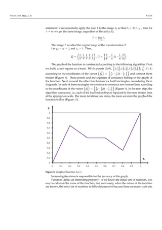
8. Fractal Fract. 2021, 5, 31 8 of 14
geometric interpretation of the construction of this set. Let the graph of the function F0(x)
be broken, connecting series points:
(0; 0), (q01; g01),
1
∑
i=0
qi1;
1
∑
i=0
gi1
,
2
∑
i=0
qi1;
2
∑
i=0
gi1
,
3
∑
i=0
qi1;
3
∑
i=0
gi1
,
4
∑
i=0
qi1;
4
∑
i=0
gi1
= (1; 1).
Graph of the function F1(x) is broken, connecting series points:
(0; 0), (q01q02; g01g02),
q01
1
∑
i=0
qi2; g01
1
∑
i=0
gi2
,
q01
2
∑
i=0
qi2; g01
2
∑
i=0
gi2
,
q01
3
∑
i=0
qi2; g01
3
∑
i=0
gi2
,
q01
4
∑
i=0
qi2; g01
4
∑
i=0
qi2
= (q01; g01);
(q01 + q11q02; g01 + g11g02),
q01 + q11
1
∑
i=0
qi2; g01 + g11
1
∑
i=0
gi2
,
q01 + q11
2
∑
i=0
qi2; g01 + g11
2
∑
i=0
gi2
,
q01 + q11
3
∑
i=0
qi2; g01 + g11
3
∑
i=0
gi2
,
q01 + q11
4
∑
i=0
qi2; g01 + g11
4
∑
i=0
qi2
=
1
∑
i=0
qi1;
1
∑
i=0
gi1
;
2
∑
i=0
qi1 + q31q02;
2
∑
i=0
gi1 + g31g02
,
2
∑
i=0
qi1 + q31
1
∑
i=0
qi2;
2
∑
i=0
gi1 + g31
1
∑
i=0
gi2
,
2
∑
i=0
qi1 + q31
2
∑
i=0
qi2;
2
∑
i=0
gi1 + g31
2
∑
i=0
gi2
,
2
∑
i=0
qi1 + q31
3
∑
i=0
qi2;
2
∑
i=0
gi1 + g31
3
∑
i=0
gi2
,
2
∑
i=0
qi1 + q31
4
∑
i=0
qi2;
2
∑
i=0
qi1 + g31
4
∑
i=0
qi2
=
3
∑
i=0
qi1;
3
∑
i=0
gi1
;
3
∑
i=0
qi1 + q41q02;
3
∑
i=0
gi1 + g41g02
,
3
∑
i=0
qi1 + q41
1
∑
i=0
qi2;
3
∑
i=0
gi1 + g41
1
∑
i=0
gi2
,
3
∑
i=0
qi1 + q41
2
∑
i=0
qi2;
3
∑
i=0
gi1 + g41
2
∑
i=0
gi2
,
3
∑
i=0
qi1 + q41
3
∑
i=0
qi2;
3
∑
i=0
gi1 + g41
3
∑
i=0
gi2
,
3
∑
i=0
qi1 + q41
4
∑
i=0
qi2;
3
∑
i=0
qi1 + g41
4
∑
i=0
qi2
= (1; 1),
i.e., F1(x) =
4
∪
i=0
Ti(F0(x)). These points are uniquely determined by the vectors Q and G,
and they belong to the interior of the square [0; 1] × [0; 1]. We say that the transformation
T is performed over the segments of the broken F0(x). With each of the segments of the
obtained broken F1(x), which are not segments of constancy, we do the same (we perform
the transformation T on them). Continuing this process, we obtain a functional sequence
(Fn(x)) such that:
Fn(x) = T(Fn−1(x)) =
4
∪
i=0
Ti(Fn−1(x)).
Thus, according to Banach’s theorem (the theorem was formulated and proved in 1922
by Stefan Banach and is one of the most classical and fundamental theorems of functional
analysis), there is a class of mappings—these are compressive mappings. A well-known

9. Fractal Fract. 2021, 5, 31 9 of 14
statement: if we repeatedly apply the map T to the image F0 so that Fi = T(Fi−1), then for
i → ∞ we get the same image, regardless of the initial F0:
F = lim
i→∞
Fi.
The image F is called the original image of the transformation T.
Let qij = qi = 1
5 and εn = 1. Then,
Q =
1
5
;
1
5
;
1
5
;
1
5
;
1
5
, G =
3
4
; −
1
4
; 0; −
1
4
;
3
4
.
The graph of the function is constructed according to the following algorithm. First,
we build a unit square as a basis. We fix points (0; 0),
1
5 ; 3
4
, 2
5 ; 2
4
, 3
5 ; 2
4
,
4
5 ; 1
4
, (1; 1)
according to the coordinates of the vector
→
g1
=
n
3
4 ; −1
4 ; 0; −1
4 ; 3
4
o
and connect them
broken (Figure 8). These points and the segment of constancy belong to the graph of
the function. Next, around the other four broken we build rectangles, considering them
diagonals. In each of these rectangles we continue to construct new broken lines according
to the coordinates of the vector
→
g2
=
n
3
4 ; −1
4 ; 0; −1
4 ; 3
4
o
(Figure 9). In the next step, the
algorithm is repeated, i.e., each of the four broken lines is replaced by five new broken lines
at the appropriate scale. The more iterations you make, the more accurate the graph of the
function will be (Figure 10).
Figure 8. Graph of function F0(x).
Increasing iterations is responsible for the accuracy of the graph.
Function (2) has an interesting property—if we know the initial sets of numbers, it is
easy to calculate the value of the function, but, conversely, when the values of the function
are known, the initial set of numbers is difficult to recover because there are many such sets.

10. Fractal Fract. 2021, 5, 31 10 of 14
Figure 9. Graph of function F1(x).
Figure 10. Graph of function F15(x).
Another special property of this function is the manifestation of self-similar properties
of the graph of the function depending on the parameter at intervals where the function
is not constant, i.e., the graph of the function Γf = {(x, f (x)), x ∈ [0, 1]} is a self-similar
set and
Γ = ∪
i∈A5, i6=2
ϕi(Γ), where ϕk(Γ) 6= ϕp(Γ), k 6= p,
ϕi :
x0 = 1
5 x + i
5 ,
y0 = gi1y + γi1
.
This allows for encoding information faster, thus increasing the efficiency of data
transmissions through communication channels.
The process of encoding information requires a lot of calculations. Large volumes
of iterations are performed to search for self-similar fragments in the image. Therefore,
compressing a single image takes a long time. In this case, the more iterations there are to
make, the more accurate the result will be.

11. Fractal Fract. 2021, 5, 31 11 of 14
Decoding a fractal image is also an iterative process, although it takes little time, as
all such objects are searched for in the encoding process. All you need to do is refine the
fractal codes by transforming them into the original image. However, if you do not know
the image encoding algorithm, the decoding process will be very cumbersome and time
consuming.
Here are some examples of fractal encoding with given initial sets of digits for a given
image f:
1. For Q-cylinders, the digits 0 and 1 are allowed, i.e., the image will be divided into
cylinders ∆0, ∆1, ∆00, ∆01, ∆10, ∆11, . . .. Then, for the second identical image, as a result
of affine transformations, the brightness distribution will contain G-cylinders with
numbers 0 and 1, i.e., the image of the set C1 ≡ C[Q∗
5; {0, 1}] is the segment
0; 3
4
(Figure 11);
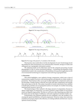
2. For Q-cylinders, the digits 1 and 3 are allowed, i.e., the image will be divided into
cylinders ∆1, ∆3, ∆11, ∆13, ∆31, ∆33, . . .. Then, for the second identical image, as a result
of affine transformations, the brightness distribution will contain G-cylinders with
numbers 1 and 3, i.e., the digits of the set C2 ≡ C[Q∗
5; {1, 3}] are a set of Cantor type
C3 ≡ C[G∗
5 ; {1, 3}] (it is a set of not deleted points; it is possible to define the relation
of this set to unit interval through the general length of the removed subintervals)
(Figure 12);
3. For Q-cylinders, the digits 1,2 and 3 are allowed, i.e., the image will be divided into
cylinders ∆1, ∆2, ∆3, ∆11, ∆12, ∆13, ∆21, ∆22, ∆23, ∆31, ∆32, ∆33, . . .. Then, for the second
identical image, as a result of affine transformations, the brightness distribution will
contain G-cylinders with digits 1,2 and 3, i.e., the image C4 ≡ C[Q∗
5; {1, 2, 3}] is the
set E = C3 ∪ M (Figure 13), where C3 is a set of Cantor type and M is a discrete subset
of the set of five-rational numbers:
M =
n
y : y = ∆
G∗
5
α1α2...αm−12(0)
, αi ∈ {1, 3}, m ∈ N
o
;
4. For Q-cylinders, the digits 0 and 4 or 1 and 3 are allowed. Then, for the second
identical image, as a result of affine transformations, the brightness distribution will
contain G-cylinders with digits 1,2,3,4, if the digits 0 and 4 or 1 and 3 are allowed
for Q-cylinders, then the image of the set of Cantor type C5 ≡ C[G∗
5 ; Vn] (Figure 14),
where
Vn =
{0, 4}, i f n = 1(mod 3),
{1, 3}, i f n 6= 1(mod 3),
is a set of Cantor type of Lebesgue zero measure.
Figure 11. The image of the plural C1.

12. Fractal Fract. 2021, 5, 31 12 of 14
Figure 12. The image of the plural C2.
Figure 13. The image of the plural C4.
Figure 14. The image of the plural C5: G-cylinders of the 3rd rank.
This function class model allows for the development of a new fractal image encod-
ing method for data transmission over communication channels, storage on media and
subsequent use in geographic information systems.
The obtained results can be effectively used for the computer processing of aerial
photographs in GIS of various functional purposes. A promising development of this
mathematical model is the consideration of the problems of its practical application in GIS
of environmental monitoring for compression and archiving of geospatial data.
4. Discussion
This article highlights a new method of image compression, which uses a class of
nonmonotonic singular functions with fractal properties and depends on a finite number of
parameters. These features allow you to get excellent digital data compression ratios and
fast decoding. Another feature is that the size of the data after compression will actually
take up less space in the file. This makes it possible to transfer information from satellites
to Earth faster and then use it in geospatial systems, for example, for weather forecasting,
studying Earth resources, and so on.
The disadvantage of this method is the large amount of computation, because to
obtain a high degree of compression, you need to perform a large number of conversions,
which can degrade image quality. The data we will receive after unpacking may differ from
the initial ones, but the degree of difference will not be significant with their further use.
Unfortunately, the proposed methods do not completely solve the problem of in-
creasing the speed and efficiency of fractal compression. However, today, more and more
scientists are trying to improve the efficiency of existing methods and find new ways to
optimize fractal encoding.

13. Fractal Fract. 2021, 5, 31 13 of 14
5. Conclusions
Mathematical models of the effective use of fractal functions for compression (encod-
ing) of raster images are covered. There are already a large number of existing models using
functions with a complex local structure, but they also need to be improved. Functions
with fractal properties, unlike conventional functions, help to efficiently encode data and
solve complex problems in various areas of human activity. Such functions are given by
a recursive formula. Their generation takes a long time, which provides a high degree
of compression, but is time consuming. Unpacking the image is easier, because the main
work has already been done during encoding and it remains only with the help of known
fractal codes to return the raster image. The obtained results allow one to create a suffi-
ciently reliable mathematical support for the process of compression of various graphic
information and to improve existing methods.
We see prospects for further research in constructing a family of functions with fractal
properties, using different systems of encoding real numbers, and their application to create
reliable and advanced methods of encoding spatial data, their storage, processing and
representation. This will create a single information space and provide ample opportunities
for systematic analysis of information for effective environmental quality management and
ensuring the safety of life.
Author Contributions: Conceptualization, O.S. and O.L.; methodology, O.S., O.L. and O.B.; valida-
tion, O.B. and O.L.; formal analysis, J.N. and R.K.; investigation, J.N. and R.K.; writing—original
draft preparation, O.B. and R.K.; writing—review and editing, O.S. and O.L. All authors have read
and agreed to the published version of the manuscript.
Funding: This research received no external funding.
Institutional Review Board Statement: Not applicable.
Informed Consent Statement: Not applicable.
Acknowledgments: The authors would like to thank the editor and the referees for his/her careful
reading and valuable comments.
Conflicts of Interest: The authors declare that there is no conflict of interest.
References
1. Barnsley, М.; Anson, L. Fractal image compression. World PC 1992, 10, 52–58.
2. Selmon, D. Compression of Data, Images and Sounds; Technosphere: Moscow, Russia, 2004; p. 368.
3. Vatolin, D.; Ratushniak, A.; Smyrnov, М.; Yukin, V. Data Compression Methods; Dialogue–MIPI: Moscow, Russia, 2002; p. 381.
4. Barnsley, M.F.; Sloan, A.D.; Iterated Systems, Inc. Methods and Apparatus for Image Compression by Iterated Function System.
U.S. Patent 4,941,193, 10 July 1990.
5. Jacquin, A. Image encoding based on a fractal theory of iterated contractive image transformations. IEEE Trans. Image Process.
1992, 1, 18–30. [CrossRef] [PubMed]
6. Fisher, Y.; Jacobs, E.W.; Boss, R.D. Fractal image compression using iterated transform. Nosc Tech. Rep. 1991, 1408, 1122–1128.
7. Vynokurov, S. An efficient fractal image compression algorithm using spatially sensitive hashing. Open Educ. 2006, 4, 62–70.
8. Vatolin, D. Using DKT to accelerate fractal image compression. Programming 1999, 3, 51–57.
9. Kominek, J. Algorithm for Fast Fractal Image Compression. Proc. Spiedigit. Video Compress. Algor. Technol. 1995, 2419, 296–305.
10. Welstead, S. Self-Organizing Neural Network Domain Classification for Fractal Image Encoding. In Proceedings of the IASTED
International Conference “Artificial Intelligence and Soft Computing”, Banff, AB, Canada, 27 July–1 August 1997; pp. 248–251.
11. Vences, L.; Rudomin, I. Genetic Algorithms for Fractal Image and Image Sequence Compression; Institute of Technology, University of
Monterrey: San Pedro Garza García, Mexico, 1997; p. 10.
12. Xi, L.; Zhang, L. A Study of Fractal Image Compression Based on an Improved Genetic Algorithm. Int. J. Nonlinear Sci. 2007, 3,
116–124.
13. Hassaballah, M.; Makky, M.M.; Mahdy, Y.B. A Fast Fractal Image Compression Method Based Entropy. Electron. Lett. Comput. Vis.
Image Anal. 2005, 5, 30–40. [CrossRef]
14. Zubko, R. Compression of images by fractal method. East. Eur. J. Adv. Technol. 2014, 6, 23–28.
15. Maidaniuk, V.; Lishchuk, О.; Korol, D. Aspects of optimizing the speed of fractal image compression. Optoelectron. Inf. Energy
Technol. 2017, 1, 24–32.
16. Podchashynskyi, Y.; Khaustovych, О. Research of methods of fractal compression of video images with measuring information
transmitted by computer networks. Bull. Zhstu. Ser. Tech. Sci. 2018, 1, 149–154.

14. Fractal Fract. 2021, 5, 31 14 of 14
17. Barabash, O.; Laptiev, O.; Tkachev, V.; Maystrov, O.; Krasikov, O.; Polovinkin, I. The Indirect method of obtaining Estimates of the
Parameters of Radio Signals of covert means of obtaining Information. Int. J. Emerg. Trends Eng. Res. (IJETER) 2020, 8, 4133–4139.
[CrossRef]
18. Barabash, O.; Laptiev, O.; Kovtun, O.; Leshchenko, O.; Dukhnovska, K.; Biehun, A. The Method dynavic TF-IDF. Int. J. Emerg.
Trends Eng. Res. (IJETER) 2020, 8, 5713–5718.
19. Rakushev, M.; Permiakov, O.; Tarasenko, S.; Kovbasiuk, S.; Kravchenko, Y.; Lavrinchuk, O. Numerical Method of Integration
on the Basis of Multidimensional Differential-Taylor Transformations. In Proceedings of the 2019 IEEE International Scientific-
Practical Conference Problems of Infocommunications, Science and Technology (PIC ST), Kyiv, Ukraine, 8–11 October 2019; pp.
675–678.
20. Kravchenko, Y.; Leshchenko, O.; Dakhno, N.; Trush, O.; Makhovych, O. Evaluating the effectiveness of cloud services. In
Proceedings of the 2019 IEEE International Conference on Advanced Trends in Information Theory (ATIT), Kyiv, Ukraine, 18–20
December 2019; pp. 120–124.
21. Yevseiev, S.; Korolyov, R.; Tkachov, A.; Laptiev, O.; Opirskyy, I.; Soloviova, O. Modification of the algorithm (OFM) S-box, which
provides increasing crypto resistance in the post-quantum period. Int. J. Adv. Trends Comput. Sci. Eng. (IJATCSE) 2020, 9,
8725–8729.
22. Savchenko, V.; Laptiev, O.; Kolos, O.; Lisnevskyi, R.; Ivannikova, V.; Ablazov, I. Hidden Transmitter Localization Accuracy Model
Based on Multi-Position Range Measurement. In Proceedings of the 2020 IEEE 2nd International Conference on Advanced Trends
in Information Theory (IEEE ATIT 2020), Kyiv, Ukraine, 25–27 November 2020; pp. 246–251.
23. Mandelbrot, B. Fractals: Form, Chance, and Dimension; W. H. Freeman and Company: San Francisco, CA, USA, 1977; p. 352.
24. Mandelbrot, B. Fractal Geometry of Nature; W.H. Freeman: San Francisco, CA, USA, 1982.
25. Pratsiovytyi, M. Fractal Approach in Singular Distribution Studies; NPU MP Draghomanova: Kyiv, Ukraine, 1998; p. 296.
26. Zhykharieva, J.; Pratsiovytyi, М. Representation of numbers by means of the Luroth series: The basics of the metric theory. Nauk.
Chasopys. Nats. Ped. Univ. Dragomanova, Ser. 1 Fiz. Mat. Nauk. 2008, 9, 200–211.
27. Baranovskyi, О.; Pratsiovytyi, М.; Torbin, H. Ostrogradsky–Sierpinski–Pierce series and their applications. In Academy Book
Production; Naukova Dumka: Kyiv, Ukraine, 2013; p. 268.
28. Pratsiovytyi, М. Non-Cantor images of real numbers as trivial recodings of Cantor numbers. Collect. Work. Inst. Math. Natl. Acad.
Sci. Ukr. 2017, 14, 167–188.
29. Pratsiovytyi, М.; Svynchuk, O. Spread of values of a Cantor-type fractal continuous nonmonotone function. J. Math. Sci. 2019,
240, 342–357. [CrossRef]
30. Falconer, K.J. Fractal geometry. Mathematical Foundations and Applications, 2nd ed.; Wiley: Chichester, UK, 2003; p. 337.