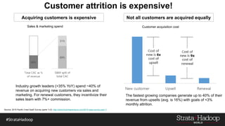
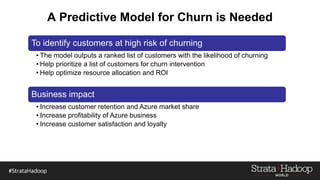
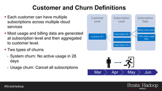
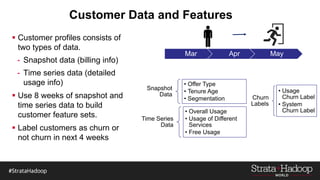
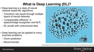
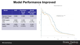
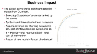
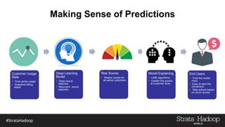
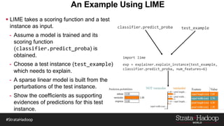
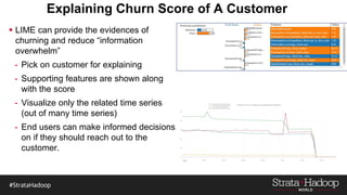
Predicting Azure Churn with
Deep Learning and Explaining
Predictions with LIME
Feng Zhu (Speaker)
Chao Zhong
Shijing Fang
Ryan Bouchard
Val Fontama (Speaker)
 Azure customers and churn
 Customer data and features
 Current ML pipelines and challenges
 Apply deep learning to improve model performance
 Explain model predictions using LIME
Azure Customers and Churn
Customer attrition is expensive!
Industry growth leaders (>35% YoY) spend ~40% of
revenue on acquiring new customers via sales and
marketing. For renewal customers, they incentivize their
sales team with 7%+ commission.
The fastest growing companies generate up to 40% of their
revenue from upsells (avg. is 16%) with goals of <3%
monthly attrition.
Not all customers are acquired equallyAcquiring customers is expensive
Sales & marketing spend Customer acquisition cost
Source: 2015 Pacific Crest SaaS Survey (parts 1+2): http://www.forentrepreneurs.com/2015-saas-survey-part-1/
A Predictive Model for Churn is Needed
To identify customers at high risk of churning
• The model outputs a ranked list of customers with the likelihood of churning
• Help prioritize a list of customers for churn intervention
• Help optimize resource allocation and ROI
Business impact
• Increase customer retention and Azure market share
• Increase profitability of Azure business
• Increase customer satisfaction and loyalty
Customer Features and ML Pipelines
Customer and Churn Definitions
Subscription
Data
Subscription
Level
Customer
Level
Customer ID 1
Subscription ID 1
Billing status data
Time series usage
data…
Subscription ID n
 Each customer can have multiple
subscriptions across multiple cloud
services
 Most usage and billing data are generated
at subscription level and then aggregated
to customer level.
 Two types of churns
- System churn: No active usage in 28
days
- Usage churn: Cancel all subscriptions
Mar Apr May Jun
Mar Apr May
Customer Data and Features
Snapshot
Data
• Offer Type
• Tenure Age
• Segmentation
Time Series
Data
• Overall Usage
• Usage of Different
Services
• Free Usage
Churn
Labels
• Usage
Churn Label
• System
Churn Label
 Customer profiles consists of
two types of data.
- Snapshot data (billing info)
- Time series data (detailed
usage info)
 Use 8 weeks of snapshot and
time series data to build
customer feature sets.
 Label customers as churn or
not churn in next 4 weeks
Feature Extraction from Time Series Data
Time Series
(20+)
• FreeUsage
• Usage of Cloud Services
• …
Extraction
Functions
(20+)
• Min Max Mean SD Median
• Number of Zero Values
• Slope
• Sum of Last Interval Values
• …
Extracted
Features
(400+)
• FreeUsage.min
• TotalUnits.max
• …
…
Customer ID 1
Churn V1 ML Pipeline
Customer
Data
• Time series
usage
• Snapshot billing
status
Feature
Engineering
• Extract features
from time series
• Combine all
features together
Random
Forest Model
• Classification
model
• 400+ features
Churn Risk
Scores
• Weekly scores for
all active customers
End Users
• Take actions
based on
prediction scores
1.“Feature explosion?” – As we increase # of time series, features extracted from time series
will grow exponentially.
1
2
3
3. “Should I trust model/scores?” - If end users do not trust a model or a prediction, they will
not use it
2. “Squeeze more juice?” – Can we further improve the model performance?
Churn V2 ML Pipeline
Customer Usage
Data
• Time series usage
• Snapshot billing
status
Deep Learning
Model
• Deep neural
networks
• Recurrent neural
networks
Risk Scores
• Weekly scores for all
active customers
Model Explaining
• LIME algorithms
• Explain the scores
at customer level
End Users
• Trust the model
more
• Easy to start the
conversion
• Take actions based
on churn scores
1.Deep learning model – 1) “automated” feature engineering 2) boosts prediction accuracy
1 2
2. LIME – An interface to explain model and predictions to end users
Deep Learning Models
What is Deep Learning (DL)?
 Deep learning is a class of neural
network based ML algorithms
- Transform raw inputs through multiple
layers of neural networks
- “unreasonably effective” in
speech/image recognition and NLP.
- DL excels with unstructured data
 Deep learning can be applied to many
business problems.
- Churn prediction
- Recommender
https://blogs.microsoft.com/next/2016/01/25/microsoft-releases-cntk-its-open-source-deep-learning-toolkit-on-git
Overview of DL Model Architecture
DNN Layer 1
DNN Layer 2
DNN Layer 3
DNN Layer 4
DNN Layer 5
RNN Layer 1
RNN Layer 2
Output Layer
Static Feature
Input
Time Series Input
Merge Layers
DNN Layer 6
 The model is a “hybrid” model consisting of
two types of neural networks.
- Deep neural networks (DNN) layers
- Takes static features as input
- Fully connected MLP with add-ons
- Recurrent neural networks (RNN) layers
- Takes time series as input
- Long Short Term Memory
(LSTM) networks
“In Deep Learning, Architecture Engineering is the
New Feature Engineering.”
DNN Layers (Left Path)
Output Layer
 Five identical DNN layers are stacked to
transform static features.
- Input dimension of DNN layer 1 equals
input dimension of static feature input
- DNN 2-5 have the same input and output
dimensions
- Batch normalization layer is for faster
convergence and “gradient vanishing”
mitigation
- Highway-like structure is to mitigate
“gradient vanishing” and improve accuracy
- The output of DNN layers is the merged
output from each layer
DNN Layer 1
…
DNN Layer 5
Dense Layer
Batch Normalization
Activation Layer
Merge Layer (concat)
Static Feature Input
RNN Layers (Right Path)
h1 h2 … h5
…
…
…
LSTM Layer 1
Time Series Input
LSTM Layer 2
x1 x2 … x56
 Two identical RNN (LSTM) layers are
stacked to transform time series data.
- The input dimension is 18*56. (18 time
series and 56 time steps).
- Each LSTM layer has 128*56 hidden
states. (128 hidden nodes and 56 time
steps)
- Highway-like structure is also added to
mitigate “gradient vanishing” and improve
accuracy
- The final output of RNN layers is the
merged states from the last time step.
Model Performance Improved
Model AUC Precision-
Recall
AUC
Recall
(@Precision
=0.562)
Random Forest
(V1 model)
0.836 0.325 0.283
DNN Layers
only
0.854
(+1.8%)
0.352
(+2.7%)
0.32
(+3.7%)
DNN + RNN
Layers
0.863
(+2.7%)
0.383
(+5.8%)
0.343
(+6%)
Business Impact
 The payout curve shows significant potential
margin from DL model.
- Select top X percent of customer ranked by
the scores
- Apply churn intervention to these customers
- Assume revenue per churning customer is
$m, cost of intervention per customer is $n
- Y = Payout = total revenue saved – total
cost of intervention
- Payout of new model - Payout of old model
Explaining Model Predictions Using LIME
Customer Usage
Data
• Time series usage
• Snapshot billing
status
Deep Learning
Model
• Deep neural
networks
• Recurrent neural
networks
Risk Scores
• Weekly scores for
all active customers
Model Explaining
• LIME algorithms
• Explain the scores
at customer level
End Users
• Trust the model
more
• Easy to start the
conversion
• Take actions based
on churn scores
LIME Algorithm
 LIME is an interface between scores and
end users.
- Local Interpretable Model-agnostic
Explanations
- Use a simple model to approximate the
scoring logic of a black-box classifier
- Fit the original classifier locally using
sparse linear models through sampling
for local exploration
An Example Using LIME
 LIME takes a scoring function and a test
instance as input.
- Assume a model is trained and its
scoring function
(classifier.predict_proba) is
obtained.
- Choose a test instance (test_example)
which needs to explain.
- A sparse linear model is built from the
perturbations of the test instance.
- Show the coefficients as supporting
evidences of predictions for this test
instance.
Explaining Churn Score of A Customer
 LIME can provide the evidences of
churning and reduce “information
overwhelm”
- Pick on customer for explaining
- Supporting features are shown along
with the score
- Visualize only the related time series
(out of many time series)
- End users can make informed decisions
on if they should reach out to the
customer.
Summary
Lessons Learned and Future Plans
Lessons learned
- “In Deep Learning, Architecture Engineering is the New Feature
Engineering.”
- Quantify the business value to motivate stakeholders
- Making sense of predictions helps operationalize the model.
Future Plans
- Explore other network architectures for faster training and higher accuracy
- Incorporate reinforcement learning to recommend the best churn
intervention action
Thanks! Questions?

Predicting Azure Churn with Deep Learning and Explaining Predictions with LIME

  • 1.
    Predicting Azure Churnwith Deep Learning and Explaining Predictions with LIME Feng Zhu (Speaker) Chao Zhong Shijing Fang Ryan Bouchard Val Fontama (Speaker)
  • 2.
     Azure customersand churn  Customer data and features  Current ML pipelines and challenges  Apply deep learning to improve model performance  Explain model predictions using LIME
  • 3.
  • 4.
    Customer attrition isexpensive! Industry growth leaders (>35% YoY) spend ~40% of revenue on acquiring new customers via sales and marketing. For renewal customers, they incentivize their sales team with 7%+ commission. The fastest growing companies generate up to 40% of their revenue from upsells (avg. is 16%) with goals of <3% monthly attrition. Not all customers are acquired equallyAcquiring customers is expensive Sales & marketing spend Customer acquisition cost Source: 2015 Pacific Crest SaaS Survey (parts 1+2): http://www.forentrepreneurs.com/2015-saas-survey-part-1/
  • 5.
    A Predictive Modelfor Churn is Needed To identify customers at high risk of churning • The model outputs a ranked list of customers with the likelihood of churning • Help prioritize a list of customers for churn intervention • Help optimize resource allocation and ROI Business impact • Increase customer retention and Azure market share • Increase profitability of Azure business • Increase customer satisfaction and loyalty
  • 6.
  • 7.
    Customer and ChurnDefinitions Subscription Data Subscription Level Customer Level Customer ID 1 Subscription ID 1 Billing status data Time series usage data… Subscription ID n  Each customer can have multiple subscriptions across multiple cloud services  Most usage and billing data are generated at subscription level and then aggregated to customer level.  Two types of churns - System churn: No active usage in 28 days - Usage churn: Cancel all subscriptions Mar Apr May Jun
  • 8.
    Mar Apr May CustomerData and Features Snapshot Data • Offer Type • Tenure Age • Segmentation Time Series Data • Overall Usage • Usage of Different Services • Free Usage Churn Labels • Usage Churn Label • System Churn Label  Customer profiles consists of two types of data. - Snapshot data (billing info) - Time series data (detailed usage info)  Use 8 weeks of snapshot and time series data to build customer feature sets.  Label customers as churn or not churn in next 4 weeks
  • 9.
    Feature Extraction fromTime Series Data Time Series (20+) • FreeUsage • Usage of Cloud Services • … Extraction Functions (20+) • Min Max Mean SD Median • Number of Zero Values • Slope • Sum of Last Interval Values • … Extracted Features (400+) • FreeUsage.min • TotalUnits.max • … … Customer ID 1
  • 10.
    Churn V1 MLPipeline Customer Data • Time series usage • Snapshot billing status Feature Engineering • Extract features from time series • Combine all features together Random Forest Model • Classification model • 400+ features Churn Risk Scores • Weekly scores for all active customers End Users • Take actions based on prediction scores 1.“Feature explosion?” – As we increase # of time series, features extracted from time series will grow exponentially. 1 2 3 3. “Should I trust model/scores?” - If end users do not trust a model or a prediction, they will not use it 2. “Squeeze more juice?” – Can we further improve the model performance?
  • 11.
    Churn V2 MLPipeline Customer Usage Data • Time series usage • Snapshot billing status Deep Learning Model • Deep neural networks • Recurrent neural networks Risk Scores • Weekly scores for all active customers Model Explaining • LIME algorithms • Explain the scores at customer level End Users • Trust the model more • Easy to start the conversion • Take actions based on churn scores 1.Deep learning model – 1) “automated” feature engineering 2) boosts prediction accuracy 1 2 2. LIME – An interface to explain model and predictions to end users
  • 12.
  • 13.
    What is DeepLearning (DL)?  Deep learning is a class of neural network based ML algorithms - Transform raw inputs through multiple layers of neural networks - “unreasonably effective” in speech/image recognition and NLP. - DL excels with unstructured data  Deep learning can be applied to many business problems. - Churn prediction - Recommender https://blogs.microsoft.com/next/2016/01/25/microsoft-releases-cntk-its-open-source-deep-learning-toolkit-on-git
  • 14.
    Overview of DLModel Architecture DNN Layer 1 DNN Layer 2 DNN Layer 3 DNN Layer 4 DNN Layer 5 RNN Layer 1 RNN Layer 2 Output Layer Static Feature Input Time Series Input Merge Layers DNN Layer 6  The model is a “hybrid” model consisting of two types of neural networks. - Deep neural networks (DNN) layers - Takes static features as input - Fully connected MLP with add-ons - Recurrent neural networks (RNN) layers - Takes time series as input - Long Short Term Memory (LSTM) networks “In Deep Learning, Architecture Engineering is the New Feature Engineering.”
  • 15.
    DNN Layers (LeftPath) Output Layer  Five identical DNN layers are stacked to transform static features. - Input dimension of DNN layer 1 equals input dimension of static feature input - DNN 2-5 have the same input and output dimensions - Batch normalization layer is for faster convergence and “gradient vanishing” mitigation - Highway-like structure is to mitigate “gradient vanishing” and improve accuracy - The output of DNN layers is the merged output from each layer DNN Layer 1 … DNN Layer 5 Dense Layer Batch Normalization Activation Layer Merge Layer (concat) Static Feature Input
  • 16.
    RNN Layers (RightPath) h1 h2 … h5 … … … LSTM Layer 1 Time Series Input LSTM Layer 2 x1 x2 … x56  Two identical RNN (LSTM) layers are stacked to transform time series data. - The input dimension is 18*56. (18 time series and 56 time steps). - Each LSTM layer has 128*56 hidden states. (128 hidden nodes and 56 time steps) - Highway-like structure is also added to mitigate “gradient vanishing” and improve accuracy - The final output of RNN layers is the merged states from the last time step.
  • 17.
    Model Performance Improved ModelAUC Precision- Recall AUC Recall (@Precision =0.562) Random Forest (V1 model) 0.836 0.325 0.283 DNN Layers only 0.854 (+1.8%) 0.352 (+2.7%) 0.32 (+3.7%) DNN + RNN Layers 0.863 (+2.7%) 0.383 (+5.8%) 0.343 (+6%)
  • 18.
    Business Impact  Thepayout curve shows significant potential margin from DL model. - Select top X percent of customer ranked by the scores - Apply churn intervention to these customers - Assume revenue per churning customer is $m, cost of intervention per customer is $n - Y = Payout = total revenue saved – total cost of intervention - Payout of new model - Payout of old model
  • 19.
  • 20.
    Customer Usage Data • Timeseries usage • Snapshot billing status Deep Learning Model • Deep neural networks • Recurrent neural networks Risk Scores • Weekly scores for all active customers Model Explaining • LIME algorithms • Explain the scores at customer level End Users • Trust the model more • Easy to start the conversion • Take actions based on churn scores
  • 21.
    LIME Algorithm  LIMEis an interface between scores and end users. - Local Interpretable Model-agnostic Explanations - Use a simple model to approximate the scoring logic of a black-box classifier - Fit the original classifier locally using sparse linear models through sampling for local exploration
  • 22.
    An Example UsingLIME  LIME takes a scoring function and a test instance as input. - Assume a model is trained and its scoring function (classifier.predict_proba) is obtained. - Choose a test instance (test_example) which needs to explain. - A sparse linear model is built from the perturbations of the test instance. - Show the coefficients as supporting evidences of predictions for this test instance.
  • 23.
    Explaining Churn Scoreof A Customer  LIME can provide the evidences of churning and reduce “information overwhelm” - Pick on customer for explaining - Supporting features are shown along with the score - Visualize only the related time series (out of many time series) - End users can make informed decisions on if they should reach out to the customer.
  • 24.
  • 25.
    Lessons Learned andFuture Plans Lessons learned - “In Deep Learning, Architecture Engineering is the New Feature Engineering.” - Quantify the business value to motivate stakeholders - Making sense of predictions helps operationalize the model. Future Plans - Explore other network architectures for faster training and higher accuracy - Incorporate reinforcement learning to recommend the best churn intervention action
  • 26.

Editor's Notes

  • #4 Before we move to the deep learning and LIME part, review the v1 churn model
  • #12 Customer usage for churned customers and non-churn customers are different How to characterize the time series so that the machine learning algorithm can see the difference – through features extraction. Simple to complex features Generate superset of features
  • #14 Two new compoments DL can boost model performance by automatically extracting complex features, regular feature engineering cannot LIME can explain predictions to the end users.
  • #16 DL is the theme of conference. It has proved to be very successful in the field of image and NLP Recently, we also see its penetration in business problems.
  • #17 Recall that two types of data for customer profiling We built two paths of data transformation for two type of input data:1 For left path: 5 stacked DNN layers. For right path: 2 stacked RNN layers. No theory for building the “best” architecture = do not know the “best” features. 6. “Trial and error” is needed to find an architecture with satisfactory performance and training time.
  • #18 5 DNN layers are identical. Take one layer as an example Dense + activation layer = MLP Simply stacking a group of MLP is not working because of “gradient vanishing” issue. Batch normalization and highway are to mitigate “gradient vanishing” Output of all DNN layers are merged at the end
  • #19 RNN layers forms the right path. 2 RNN layers are identical and can be stacked together RNN takes sequential data as input and out another sequential data from hidden states. Stacking RNN: hidden states can be connected Select the last steps of LSTM and then merge with the output of DNN
  • #20  Trained two DL models, one with RNN and the other without RNN. RNN can improve the performance further. Compared to the baseline v1 model, significant increase across all performance metrics.
  • #21 Showing accuracy metrics is not enough…Justify the business value of your model! Need to quantify the business impact due to the increased accuracy. Plotting the payout curve can help. Explain the process
  • #22 Let’s review what we have done so far Trained a fancier model -> showed the improved accuracy and impact -> deployed the model -> output scores. But the model has not started to generate values until sales teams take actions based on the model output.
  • #23 Let’s review what we have done so far Trained a fancier model -> showed the improved accuracy and impact -> deployed the model -> output scores. But the model is still “up in the air” until end users take actions. Big question from end users: Can you tell me why the score is high or low for this customers? They need more info to understand the customer and start the conversation.
  • #24 LIME means … Ideas are from the group led by Prof. Guestrin in UW. (Will give a talk tomorrow on the other side of Expo room) We do not know how a black-box classifier works exactly. But we can use a simple model to approximate its scoring logic locally. The simple model serves as an explainer.
  • #25 Quickly go through an example using LIME Need two input: a scoring function and a test instance On the backend, the LIME will sample data and build linear model automatically An example output using Iris: Choose a test case with high probability to be versicolor 3 supporting evidences vs 1 non-supporting evidence
  • #26 Pick up one customer and explain Showed the supporting evidences But they are still not easy to interpret Added one more step, visualize the time series from which…
  • #28 Review what we covered in this session Shared how we built DL models, “no free lunch” Step out of ML world and think from end user perspectives. Fill the gap of the last mile between the models and end users. That is why you should do ... and do …