1. Articles
https://doi.org/10.1038/s41550-019-0933-6
1
NASA Goddard Space Flight Center, Greenbelt, MD, USA. 2
American University, Washington, DC, USA. 3
KTH Royal Institute of Technology, Stockholm,
Sweden. 4
Southwest Research Institute, San Antonio, TX, USA. *e-mail: lucas.paganini@nasa.gov
G
alileo observations showed that Europa’s mottled landscape
consists of chaotic terrains with pits, domes, platforms, irreg-
ular uplifts and lobate features1,2
. Analysis of these features,
along with radio doppler data, suggested that Europa contains a layer
of water, a silicate mantle and a metallic core3–6
. The water layer, pre-
sumed to be a thin ice sheet (~5–20 km thick) covering a putative
global ocean (~60–160 km deep), has strong implications for the dis-
covery of biosignatures beyond Earth, where the buoyant icy shell
would insulate the underlying ocean, potentially allowing it to survive
a hostile surrounding environment for geological timescales, and pre-
cluding penetration of harmful radiation below depths of ~1 m (ref. 7
).
Over the past few decades, theoretical modelling and remote
observations have revealed diverse dynamic processes that modify
Europa’s icy surface and shape its atmosphere. Jovian plasma, solar
radiation and meteoritic impacts influence the Europan environ-
ment not only by modifying the surface composition (for example,
through radiolysis) but also by populating Europa’s tenuous atmo-
sphere, where strong energetic radiation and thermal desorption
feed the atmosphere with particles stripped from its surface. These
exogenic processes yield substantial quantities of water, along with
atomic/molecular oxygen and hydrogen, and alkali metals8–11
.
Theoretical models12,13
estimate that exogenic sources of the most
abundant surface species (H2O, O2 and H2) populate the atmosphere
at rates of ~1026
–1027
molecules s–1
. Plumes, on the other hand, act
as endogenic mechanisms14
—probably driven by tidal flexing—that
sporadically feed Europa’s atmosphere with particles from the global
ocean, or intermediate liquid pockets, at rates (>1028
molecules s–1
)
that can surpass those from exogenic effects.
Estimates of water vapour on Europa (either from exogenic or
endogenic sources) have relied strongly on modelling efforts, yet
confirmation from observational data has been lacking. In 2012,
ultraviolet observations15
with the Hubble Space Telescope (HST)
found simultaneous auroral emission features of hydrogen and
oxygen in the southern hemisphere, at abundances greater than
1029
molecules s–1
, which exceeds the values expected from exo-
genic effects by factors of 100–1000. This was the first successful
detection and characterization of plume content on Europa. These
spectroscopic measurements of plume-like H and O emissions,
however, have not yet been confirmed despite numerous attempts,
making detection of these features an elusive endeavour. Recent
transit imaging16
and reanalysis of Galileo magnetic and plasma
field data have served as independent assessments of plume activ-
ity17,18
. However, the intrinsic characteristics of these observations
preclude direct determination of water.
In 2016, we began an observing programme aimed at charac-
terizing the chemical composition of Europa’s atmosphere—par-
ticularly water vapour—with the near-infrared spectrograph
(NIRSPEC) at the 10-m Keck Observatory. The key advantage of
observations at infrared wavelengths is the ability to measure H2O
(not H and O), thereby providing a direct and independent assess-
ment of water vapour in Europa’s atmosphere (see Supplementary
Fig. 1). In the nearly collisionless environment, solar excitation of
molecules (water and organics) results in the emission of infra-
red photons through decay to the ground vibrational state, either
directly (resonant fluorescence) or through branching into inter-
mediate vibrational levels (non-resonant fluorescence), allowing
these signatures to be detected using high-resolution spectroscopy.
We targeted radiative excitation of water molecules via solar excita-
tion in the 2–5.5-μm wavelength range, along with organics such as
ethane, methanol, methane, hydrogen cyanide, formaldehyde and
ammonia (depending on the instrument configuration). Our survey
consisted of 17 observations, spanning dates from February 2016
to May 2017 (see Tables 1 and 2 for details). Multiple visits were
needed to provide full longitudinal sampling and temporal coverage
to probe the possible cadence of water vapour activity, and included
some back-to-back observations of particular regions after a single
orbital period (3.55 d). We obtained disk-averaged measurements
of Europa, as defined by the instrument slit of 0.4′′ width (or 0.7′′,
depending on the night’s ‘seeing’) and spatial extract of ~1′′ along
the north–south or east–west direction.
Of the 17 observations, our results on 16 dates indicated no
detection of atmospheric emission features within sensitivity lim-
its, thus establishing a rather quiescent state. The sensitive upper
limits for water outgassing indicated column densities as low as
A measurement of water vapour amid a largely
quiescent environment on Europa
L. Paganini 1,2
*, G. L. Villanueva1
, L. Roth 3
, A. M. Mandell1
, T. A. Hurford1
, K. D. Retherford4
and M. J. Mumma 1
Previous investigations proved the existence of local density enhancements in Europa’s atmosphere, advancing the idea of a
possible origination from water plumes. These measurement strategies, however, were sensitive either to total absorption or
atomic emissions, which limited the ability to assess the water content. Here we present direct searches for water vapour on
Europa spanning dates from February 2016 to May 2017 with the Keck Observatory. Our global survey at infrared wavelengths
resulted in non-detections on 16 out of 17 dates, with upper limits below the water abundances inferred from previous esti-
mates. On one date (26 April 2016) we measured 2,095 ± 658 tonnes of water vapour at Europa’s leading hemisphere. We
suggest that the outgassing of water vapour on Europa occurs at lower levels than previously estimated, with only rare localized
events of stronger activity.
Nature Astronomy | www.nature.com/natureastronomy
2. Articles Nature Astronomy
1.3 × 10¹⁹
H2O m–2
and 2.6 × 10¹⁹
H2O m–2
(3σ) in 2016 and 2017,
respectively. One measurement, however, yielded an indication of
spectral emission suggesting the presence of water vapour on 26
April 2016 (Fig. 1), at sub-observer longitude of ~140° ± 40° (lead-
ing hemisphere), when Europa was near apocentre (true anomaly
~159–176°). The signal-to-noise ratio (SNR) of the retrieved H2O
spectrum (3.1σ) prevents us from establishing a definitive detec-
tion, yet co-addition of several spectral water lines and cross-cor-
relation analysis of the observed spectra provide further statistical
significance, corroborating the presumed water activity. Details of
the data analysis and statistical approaches can be found in the ‘Data
analysis’ section of the Methods. In Fig. 1, we show results from
observations on similar longitudes during orbits that were contem-
porary with the detection date, before (12 and 19 April) and after
(29 April), suggesting that the presence of water vapour on 26 April
2016 was an isolated event. Supplementary Figs. 2, 3, 7 and 8 show
the results from the entire observing campaign during 2016 and
2017. The measurement of water output on 26 April 2016 corre-
sponds to a mean column density of (1.4 ± 0.4) × 1019
H2O m–2
, total-
ling (7.0 ± 2.2) × 1031
molecules in the field of view subtended by our
observations on that date (~1,491 × 3,420 km2
).
With regard to other volatiles, we did not detect methanol nor eth-
aneatupperlimits(3σ)of1.9 × 1018
CH3OH m–2
and3.0 × 1017
C2H6 m–2
(that is, mixing ratios of <14.3% CH3OH and <2.2% C2H6 relative to
water on 26 April 2016). Although not restrictive, these upper limits
provide context to expected column densities resulting from plumes
and/or sputtering (1013
–1016
CH3OH m–2
and 1014
–1018
C2H6 m–2
,
based on theoretical models19
). The chosen instrument configuration
precluded us from obtaining measurements of other trace species
(mainly, HCN, CH4, NH3 and H2CO) on 26 April 2016.
Is the observed water vapour a consequence of endogenic
(plume-driven) activity or exogenic effects (sputtering, sublimation,
impacts)? We favour the first interpretation. Theoretical mod-
els provide differing results regarding the predicted water yields
from exogenic processes, with some studies estimating water col-
umn densities of ~1016
H2O m–2
(refs. 11,13,20
), while others predict
~1018
–1019
H2O m–2
(refs. 19,21
). Using this information—and not-
ing the dissimilar predictions—we identify opposing views to the
possible origin of the observed water vapour: (1) an interpretation
that suggests our water measurement (of ~1.4 × 10¹⁹
H2O m–2
) sur-
passes the mass volume expected from exogenic sources by at least
three orders of magnitude (implying an endogenic source) versus
(2) the contrasting view that the detected water levels could result
from exogenic effects. Most of these models indicate that the higher
yields are expected on Europa’s trailing hemisphere12
, yet our mea-
surement of water vapour occurred during observations of the lead-
ing hemisphere (see sub-observer longitudes in Table 2). Moreover,
most of our observations resulted in non-detections at upper lim-
its of ~1019
H2O m–2
, both on the trailing and leading hemispheres
(Fig. 2), so if one assumes that exogenic sources produce water
vapour at somewhat constant rates, we should have measured
water vapour more than once. Similarly, if one considers the
expected production rates using a simple plume model, we esti-
mate a total water production rate of (7.9 ± 2.5) × 1028
molecules s–1
(~ 2,360 ± 748 kg s–1
; see the subsection ‘Calculation of column den-
sity and production rates’ in Methods), which is at least a factor of
ten larger than global values expected from sputtering and desorp-
tion of the icy water surface12
of ~1026
–1027
molecules s–1
. Therefore,
considering that our ground-based observations are sensitive to
somewhat large amounts of water vapour rates (~1028
molecules s–1
),
the 26 April data suggest that the water vapour measured in 2016
resulted from a singular, localized event that increased the water
abundance to detectable limits (of a few 1019
H2O m–2
), as would be
the case of endogenic activity19
.
Table 1 | Atmospheric conditions during observations
Observation date and time (ut)a
RHb
(%) Windb
(mph) Mean seeing (DIMM)b
Airmassc
PWV1c
(mm) PWV2d
(mm)
3 February 2016 11:31 20 10 0.96 1.1 1.2 0.9–1.1
3 February 2016 13:14 21 0 0.96 1.1 1.0 0.9–1.1
5 February 2016 13:48 4 1 0.60 1.2 0.6 0.6–0.7
10 February 2016 11:55 18 22 0.78 1.1 0.7 1.1–1.5
12 February 2016 11:09 11 20 0.51 1.0 0.7 0.6–0.8
12 February 2016 14:17 12 15 0.51 1.4 0.6 0.6–0.8
19 February 2016 10:52 12 0 0.51 1.0 0.6 0.7–0.9
27 February 2016 11:06 5 14 0.51 1.1 0.8 0.7–0.9
12 April 2016 06:29 14 15 0.74 1.0 0.7 0.8–1.0
19 April 2016 07:46 16 3 0.55 1.1 1.2 0.9–1.1
26 April 2016 05:32 9 0 0.52 1.0 0.8 0.7–0.9
29 April 2016 08:10 6 13 0.72 1.1 1.5 1.0–1.5
11 February 2017 11:48 18 50 n/a 1.2 4.8 3.5–4.5
17 February 2017 10:47 13 11 0.49 1.5 1.4 1.0–1.2
05 March 2017 11:10 11 20 0.52 1.1 3.4 3.5–4.5
12 March 2017 10:22 30 0 n/a 1.1 3.7 4.0–6.0
15 March 2017 7:50a
26 0 0.69 1.7 2.8 3.0–4.0
19 March 2017 11:47 35 24 0.77 1.1 3.8 2.5–3.5
22 March 2017 13:29 8 6 0.59 1.4 1.6 1.8–2.2
07 May 2017 13:29 18 0 0.71 1.2 2.0 1.3–1.8
a
These values represent the midpoint of data acquisition. b
Relative humidity (RH), wind and mean seeing obtained from Maunakea Weather Center (MKWC) (http://mkwc.ifa.hawaii.edu/current/seeing/
index.cgi). c
Airmass and precipitable water vapour (PWV1) obtained from our retrieval algorithm. d
Predicted precipitable water vapour (PWV2) obtained from MKWC’s archive forecast data (http://mkwc.
ifa.hawaii.edu/forecast/mko/archive/index.cgi).
Nature Astronomy | www.nature.com/natureastronomy
3. ArticlesNature Astronomy
Once in the atmosphere, the fate of the released water mol-
ecules will depend on the solar radiation, the Jovian plasma field
and Europa’s gravitational field, leading to one (or more) of the
following mechanisms: excitation, ionization, dissociation, return
(freeze out) and/or escape. Most water molecules will return to
the surface and freeze out, due to Europa’s large escape velocity
of 2,000 m s–1
and a high sticking coefficient. It is estimated that
~42–86% of the material ejected from all exogenic and endogenic
sources returns to the surface, with models22
showing a total erosion
rate of ~0.0147 μm yr–1
. A small fraction of the plume water will be
dissociated into OH, H, O and/or H2. Electron impact dissociation,
likely to be the dominant dissociative mechanism23
, will dissociate
~1% of water or less24
. This estimate assumes a residence time of
water molecules in the atmosphere of hundreds of seconds (~887 s,
as defined by ballistic trajectories: t ≈ 2v/g, where v is the mean
molecular speed of ~ 583 m s–1
at 273 K, and g is Europa’s gravity of
1.315 m s–2
), and an electron impact dissociation rate23
on the order
of ~10–5
s–1
. HST was able to detect such a small (electron-excited)
population of H and O in December 201215
.
To put our global observations in context, we compare our most
sensitive H2O data at different Europan longitudes with HST indi-
rect estimates of water in 201215
and 201416
(see Fig. 2). We stress
that these measurements sampled different physical mechanisms,
given that previous techniques with HST were sensitive either to
total absorption or atomic emissions. With that in mind, the HST
measurements of auroral emission15
estimated a total water content
of (13 ± 3) × 1031
molecules near ~180° W, while the transit obser-
vations16
led to estimates on three different dates near ~270° W,
with values ranging (4–25) × 1031
molecules and a median value of
18 × 1031
molecules. Our infrared observations indicate upper limits
for water vapour of ~6 × 1031
at similar longitudes (that is, a factor of
2–3 lower amount of water vapour on the trailing hemisphere, using
data on 19 and 27 February 2016). Even though the positions of
active areas differ significantly—especially with the transit observa-
tions (~270° W longitude)—and the time of acquisition was differ-
ent, the HST rates of water release agree with Keck measurements
((7.0 ± 2.2) × 1031
H2O molecules) within 2σ uncertainties.
Observations at different orbital positions with respect to Jupiter
(true anomaly) allowed the study of tidal effects on the presumed
activity (see Supplementary Fig. 11). The H2O detection on 26 April
2016 by Keck and the 2012 H and O detection by HST15
occurred
near Europa’s apocentre (contrary to the HST transit observations16;
see Supplementary Fig. 4). Plume activity may be expected at certain
orbital locations if tidal cycles force active geology, and this hypoth-
esis has been foundational when attempting predictions of locus and
variation in plume activity. For instance, on Enceladus, eruptions of
plume material have been linked to tidal stresses25,
and observations
from Cassini’s Visible and Infrared Mapping Spectrometer (VIMS)
verified that tidal activity varies on an orbital timescale26
, with max-
ima near the apocentre. As mentioned already, our infrared survey
of Europa provided uniform measurements at different orbital posi-
tions, yielding temporal coverage appropriate to constrain the acti-
vation of plumes driven by tidal effects, yet results suggest no direct
evidence of repeated activity within sensitivity limits in our survey.
The latter is in line with theoretical analysis27
of hypothetical active
fractures under tidal stress that suggested no correlation between
large-scale plume activity and source location; this indicates that
the presence of active, large fractures is unlikely on Europa, in
contrast to Enceladus’s ‘tiger stripes’. Moreover, analysis of possible
source regions was hampered by the existing surface resolution
Table 2 | Results from our infrared observations including the 16 non-detections (upper limits, 3σ) and the water detection on 26
April 2016
Observation date and
time (ut)a
Time on
source
(min)
Spatial
resolution
(km2
per pixel)
Spectral
extract
(pixels)
Slit Sub-observer
longitude (° W)
TA (°) Europa
diameter
(″)
Total water
molecules
(× 1032
)b
Total water
molecules
(σ × 1032
)
3 February 2016 11:31 61 662 × 482 15 NS 17–24 347–354 0.9 <2.05 0.68
3 February 2016 13:14 97 662 × 481 15 EW 24–35 354–5 0.9 <1.60 0.53
5 February 2016 13:48 100 658 × 479 15 NS 230–240 201–204 0.9 <0.93 0.31
10 February 2016 11:55 164 653 × 475 15 NS 9–26 344–1 0.9 <1.14 0.38
12 February 2016 11:09 124 650 × 473 25 NS 209–222 184–198 1.0 <1.12 0.37
12 February 2016 14:17 64 650 × 473 25 EW 222–229 198–205 1.0 <1.09 0.36
19 February 2016 10:52 152 643 × 468 15 NS 198–215 178–196 1.0 <0.62 0.21
27 February 2016 11:06 132 639 × 465 15 NS 291–306 277–292 1.0 <0.58 0.19c
12 April 2016 06:29 105 661 × 481 15 NS 158–171 174–188 0.9 <0.76 0.25
19 April 2016 07:46 60 672 × 489 15 NS 154–160 174–181 0.9 <1.07 0.36
26 April 2016 05:32 148 684 × 497 15 NS 134–150 159–176 0.9 0.70 0.22
29 April 2016 08:10 24 690 × 502 15 NS 90–94 115–120 0.8 <1.50 0.50
11 February 2017 11:48 88 690 × 502 15 NS 257–268 19–28 0.9 <1.50 0.50
17 February 2017 10:47 32 692 × 503 15 NS 346–359 268–272 0.9 <2.30 0.77
5 March 2017 11:10 70 664 × 483 15 NS 170–175 186–191 100–105 117–120 0.9 <1.64 0.55
12 March 2017 10:22 161 655 × 476 15 NS 157–174 92–109 0.9 <1.22 0.41
15 March 2017 07:50a
46 652 × 474 15 NS 91–100 30–39 0.9 <6.99 2.33d
19 March 2017 11:47 52 648 × 471 15 NS 154–159 93–98 1.0 <1.88 0.63
22 March 2017 13:29 55 646 × 469 15 NS 105–110 48–54 1.0 <2.18 0.73
7 May 2017 13:29 92 657 × 477 15 NS 61–70 32–42 0.9 <1.21 0.40
a
All observations were taken using a KL filter (~2.9 μm), except 15 March 2017, which used an M-band filter (~5.5 μm). NS, north–south; EW, east–west; TA, true anomaly. b
Assumed rotational temperature:
50 K. Column density is Ncol (molecules m−2
) = total water/(spatial resolution × spectral extract × 106
). c
Most sensitive observation. d
Least sensitive observation.
Nature Astronomy | www.nature.com/natureastronomy
4. Articles Nature Astronomy
(~1 km per pixel, from the Galileo regional mapping campaign),
leading to limited information resulting from active geology.
Could the observed water vapour be linked to a subsurface ocean?
At present, the most direct evidence that suggests a subsurface ocean
exists on Europa was the detection of an induced magnetic field28
.
This field is likely to be produced in an electrically conductive near-
surface region (for example, a global ocean of salty water). Moreover,
geologic features have served as an indicator of the subsurface liq-
uid water ocean5
. Replication of Europa’s terrain (ridges, pits, spots)
suggests a thickness of the whole icy shell of a few kilometres up
to 40 km, formed by an elastic lithosphere of <2 km and a ductile
convecting layer from 4 to >20 km thick5
. If one considers an ice
layer ~5–20 km deep, we predict that an active vent would require
an effective area with diameter of ~120–480 m to expel 2,095 tonnes
of water vapour (see details in the subsection ‘Estimates of vent
properties’ in Methods). These values should be taken as first-order
estimates, given that we considered the ideal case scenario where
the vent was described as a cylinder. In reality, we do not know the
actual structure of Europan vent systems. Questions remain as to
whether the observed activity might originate from intermediate
liquid pockets closer to the surface, as well as to what mechanisms
are responsible for the sporadic detections. Theoretical studies have
indicated that, at low stresses and strains, ice will deform in an elas-
tic (recoverable) manner. However, at relatively large strains, the ice
would undergo irrecoverable deformation. At low temperatures this
deformation will be accomplished by brittle failure, while at higher
temperatures the result will be ductile creep29
. Hence, the observed
water vapour could issue from water pockets in the icy layer that act
as pressurized chambers whose enclosed vapour escapes to space
through narrow fissures, cracks, dikes, diapirs or a combination
of all these. Decay of radioactive nuclei and tides30
could increase
heat and internal pressure in the subsurface environment to a point
where short-lived break-ups occur, similar to water-driven mecha-
nisms like the inferred pressure chambers on Enceladus31
. Other
possible source mechanisms for such water vapour activity include
hydraulic flows32
, cryovolcanic eruptions33
and/or vertical fracture
channels along the icy sheet covering the subsurface ocean27
.
Theoretical approaches have provided valuable information
about the Europan environment, yet observational astronomy has
gathered limited details of exospheric water and other organics,
including the expected temporal variability based on model predic-
tions19
. The results of our IR survey set global (upper) limits to the
expected water vapour from exogenic sources and suggest that the
tentative detection of water vapour resulted from a sporadic event,
likely to be due to endogenic (plume-driven) activity. In fact, all
individual detection strategies and wavelength regimes used to date
have provided independent assessments that together convey the
idea that observed features on Europa are transient and likely to be
a result of plume activity (as suggested by the large number of non-
detections in our survey and recent follow-up auroral observations
with HST). However, these conclusions are strongly driven—and
hampered—by the sensitivity limits of current ground and space-
based facilities, making the detection of lower activity levels and
proper characterization of Europa’s atmosphere a complex endeav-
our with current technology. Considering these limitations, the
research presented herein has developed our understanding of water
vapour on Europa. Still, improved strategies from the ground should
pursue follow-up observations in the 2.9-μm region with upgraded
instrumentation featuring low noise detectors and higher sensitivity
to spectral lines, as well as regularly scheduled time-serial searches
for water rotational lines and organics with the Atacama Large
Millimeter/submillimeter Array. In the mid-2020s, the 30-m-class
telescopes (for example, the Thirty Meter Telescope and Extremely
Large Telescope) will provide the sensitivity and angular resolution
needed to better characterize Europa, overcoming current limita-
tions of ~10-m-class ground-based facilities in the infrared.
From space, the access to fundamental bands of water and carbon
dioxide with space assets such as the James Webb Space Telescope
SNR = 3.1SNR = 0.7
–5
0
5
10
15
Fluxdensity(relative)
SNR = 0.6
26 April 201619 April 2016 29 April 2016
–1.0 –0.5 0 0.5 1.0
Wavenumber (cm–1
)
–5
0
5
10
15
Fluxdensity(relative)
–1.0 –0.5 0 0.5 1.0
Wavenumber (cm–1
)
–5
0
5
10
15
Fluxdensity(relative)
–1.0 –0.5 0 0.5 1.0
Wavenumber (cm–1
)
Tentative water detection
–1.0 –0.5 0 0.5 1.0
Wavenumber (cm–1
)
–1.0
–0.5
0
0.5
1.0
Linearcorrelation
–1.0 –0.5 0 0.5 1.0
Wavenumber (cm–1
)
–1.0
–0.5
0
0.5
1.0
Linearcorrelation
–0.5 0 0.5 1.0
Wavenumber (cm–1
)
–1.0
–0.5
0
0.5
1.0
Linearcorrelation
–1.0
12 April 2016
–5
0
5
10
15Fluxdensity(relative)
–1.0 –0.5 0 0.5 1.0
Wavenumber (cm–1
)
–1.0
–0.5
0
0.5
1.0
Linearcorrelation
–1.0 –0.5 0 0.5 1.0
Wavenumber (cm–1
)
SNR = 1.8
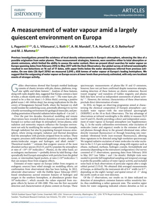
Fig. 1 | Spectra of co-added water lines in April 2016. Observations of similar longitudes during orbits that were contemporary with the detection
date, before (12 and 19 April) and after (29 April), suggest that the presence of water vapour on 26 April 2016 was an isolated event. Top: the light
blue line shows the co-added fluorescence model of the seven most significant water lines, the dark blue and red lines indicate the expected position of
Europan and terrestrial water, and the grey shaded area shows ±1σ uncertainties. Bottom: computation of the linear Pearson correlation coefficient of
a fluorescence water model and the corresponding co-added residuals. Results from all dates can be found in Supplementary Figs. 7 and 8. The central
wavenumber corresponds to the Doppler-corrected line centre of the seven most significant spectral H2O lines.
Nature Astronomy | www.nature.com/natureastronomy
5. ArticlesNature Astronomy
(JWST) (expected to be operational in the early 2020s) might permit
even more sensitive observations of water release at infrared wave-
lengths that could help to better understand the moon’s activity and
quiescent state. The JWST instruments (for example, NIRSpec inte-
gral field unit) will deliver spatial resolution on the order of 0.1′′
(~340 km) at wavelengths near 3 μm that can yield better abundance
constraints at low altitudes; in these regions, some hydrocarbons
such as ethylene, methanol and hydrogen cyanide are expected to
increase by an order of magnitude from night-to-day, while other
species like methane, acetylene and ethane might show little rela-
tive change in column densities19
. In ~2030, two major astronomi-
cal facilities, Europa Clipper and the JUpiter ICy moons Explorer
(JUICE) mission, will provide giant leaps in our understanding of
Europa and other Jovian moons. Featuring unparalleled sensitivity
and spatial resolution, these in situ observations will obtain a closer
assessmentofactiveprocessesthatshapetheatmosphere.Ultimately,
the study of fresh material released from potentially active vents
promises to further unlock the secrets of Europa, especially tantaliz-
ing in light of the existence of subsurface aqueous environments on
Europa and other ocean worlds in our Solar System.
Methods
Observing technique and strategy. Keck/NIRSPEC is a cross-dispersed echelle
grating spectrometer, which features high sensitivity and high spectral resolving
power. The cross-dispersed capability permits sampling of multiple spectral
orders, facilitating the simultaneous detection of several molecules with high
spectral resolving power (RP = λ/∆λ ≈ 25,000 with our slit configuration, where λ
is wavelength), and allowing the measurement of individual line intensities. The
high resolving power also reduces spectral confusion in crowded regions, while
improving sensitivity by reducing background emission per resolution element.
Our observing strategy involved nodding the telescope in a four-step sequence
‘ABBA’ to cancel background emissions (where A and B represent relative positions
of Europa 12′′ apart along the instrument’s slit). The data reduction and analysis
of the acquired spectral frames included flat fielding, removal of pixels affected by
high dark current and/or cosmic-ray hits, spatial and spectral rectification, and
spatial registration of individual A and B beams. The technique and data analysis
have been extensively discussed elsewhere34–37
. This is a well-established technique
that we have used effectively in the detection of water and organics in planetary
atmospheres, exoplanets and small bodies. Therefore, we applied the same concepts
from one sub-field to another sub-field in the search for water on Europa.
The analysis featured certain algorithms tailored to Europa’s high-resolution
spectral data. After combining the A and B beams from the (processed) difference
frames, which further assists in removing any residual background emission, we
extract spectra by summing 5 pixels (equal to ~1′′, or 3,250 km) in the spatial
direction and either 3 (0.4′′ ≈ 1,500 km) or 5 pixels (0.7′′ ≈ 2,500 km) for each
row in the spectral direction depending on the slit width. This yields nearly disk-
averaged measurements given Europa’s diameter of ~1′′. This strategy permitted
us to cover about 10–20° in longitude per setting (time-dependent sub-observer
W longitudes are shown in Table 2); however, the actual coverage was a factor of
~4 larger due to the slit width and its projection on Europa’s disk. Supplementary
Figs. 2 and 3 show the time-dependent longitude on the upper part of the figures,
with a colour-coded identification on each date. The shaded red areas represent the
actual slit coverage. Calibration of data was obtained through observations of flux
standard stars with the 0.720′′ × 24′′ slit configuration. We used BS4471, BS5384,
BS3982 in 2016; and BS3903, BS5685, BS4689 in 2017. For further details regarding
flux calibration, please see the Supplementary Information.
In 2016, our strategy was to measure activity during Europa’s orbit near the
apocentre and pericentre to study the possible role of tidal effects on the presumed
activity, but we also performed observations at other true anomalies (Supplementary
Fig. 4). Weather conditions outside the dome were characterized by temperatures
slightly above freezing. Image quality (seeing) was very good, as described by the
observing characteristics in Table 1: seeing DIMM <1′′, RH < 21%, wind speed < 22
mph, and low precipitable water vapour (PWV) < 1.5 mm in 2016. In 2017, we
revisited some areas of interest based on the analysis of 2016 data, and also performed
observations during eclipse and transit; however, the observing conditions in 2017
were somewhat hampered by higher humidity and PWV (up to 4.8 mm).
Data analysis. Despite the large distances between the Sun and the Jovian system,
solar radiation is an efficient excitation mechanism at relatively large heliocentric
distances—even beyond 6 au (ref. 38
)—allowing high-resolution spectroscopy
to strategically sense water through non-resonance fluorescence at infrared
wavelengths (so-called hot-band emission39
). We targeted water lines (and
organics) characterized by favourable transmission (Doppler shifted from their
terrestrial counterparts) and low contamination from reflected solar absorption
lines, which permitted sensitive measurements in the infrared.
We focused on two spectral regions: near ~2.9 μm and ~5.5 μm. The first
region allowed us to measure (hot-band) water lines resulting from (ν1 + ν3) – ν1,
(ν1 + ν2 + ν3) – (ν1 + ν2), 2ν1 – ν3, and (2ν1 + ν3) – 2ν1 at ~2.9 μm, using NIRSPEC’s
KL1 and KL2 settings. The intrinsic characteristics of the KL1 setting allowed us
to search for CH3OH and C2H6, while the KL2 setting permitted searches for CH4,
NH3, NH2, HCN and H2CO. In this Article, we report upper limits for CH3OH
and C2H6 relative to the tentative water detection on 26 April 2016, but defer the
analysis on other dates to a future publication. The second region (at ~5.5 μm)
allowed the characterization of water through the ν3 – ν2, ν1 – ν2 and (ν2 + ν3) – 2ν2
bands, using the M-wide setting; however, these observations had inferior
sensitivity due to the changing sky conditions compared with those at ~2.9 μm, so
we favoured results from observations at shorter wavelengths when available.
Analysis of Europa data accounted for intrinsic characteristics at the time of
observations, such as heliocentric distance and orbital velocity of Europa (the Swings
effect), geocentric distance and velocity (Doppler shift), and albedo (estimated).
Once the spectra were calibrated, the core of our analysis was defined by a two-
stage approach applied uniformly to the entire dataset, to minimize systematics
and human error. Calibrated spectra contained information from molecular lines
of Europa’s atmosphere and continuum, and they can be characterized by at least
four well-defined components: (1) Europa’s continuum (reflected sunlight with
Fraunhofer lines at the corresponding heliocentric velocity and geocentric velocity),
(2) signatures from the terrestrial atmosphere, (3) instrument systematics and (4)
possible Europan molecular lines (for instance, resulting from fluorescence emission).
360 270 180 90 0
Longitude (° W)
3.0
2.0
1.0
2,000
4,000
6,000
H2OWeight(tonnes)
8,000
TotalH2Omolecules(×1032
)
19 February 10 February26 April27 February
HST/STIS (auroral)
HST/STIS (transit)
Keck/NIRSPEC (this work)
Trailing hemisphere Leading hemisphere
7 May
Fig. 2 | Most sensitive estimates of water versus longitudinal coverage. Global observations of water vapour can be put in perspective to previous
localized estimates15,16
. Our results show a rather quiescent state at most longitudes, with upper limits (unfilled black circles) of ~5.8 × 1031
H2O molecules
(minimum), ~8.8 × 1031
H2O molecules (median). The tentative detection of water (filled black circle) on 26 April 2016 indicates plume content of
(7.0 ± 2.2) × 1031
H2O molecules (2,095 tonnes). Horizontal lines indicate longitudinal coverage (given by the field of view), while vertical lines represent
±1σ uncertainties. We show the median value resulting from the three measurements using transit observations16
(green triangle) and the total range
of ±1σ uncertainties (vertical line), as well as the auroral H and O results15
(blue square). The sensitivity can be hampered by factors such as the sky
conditions and (short) time on source. Supplementary Figs. 2 and 3 show an extended version with results from the complete survey.
Nature Astronomy | www.nature.com/natureastronomy
6. Articles Nature Astronomy
The first stage of analysis employed the Levenberg–Marquardt least-squares
fitting method to identify features 1–3, using synthetic modelling and noise
analysis in the calibrated data. The fitting method is an iterative process until
errors are minimized. To identify and isolate reflected solar features, we used a
model for a disk-averaged solar spectrum that combines data from the spaceborne
Atmospheric Chemistry Experiment (ACE)40
and a purely theoretical model41
.
The Atmospheric Chemistry Experiment spectrum features very high resolving
power (R ≈ 1 × 10⁵
from 750–6,000 cm−1
); this model is then normalized to
Europa’s continuum in the combined spectrum (Supplementary Fig. 5 shows the
continuum flux levels) and fitted with a transmittance function synthesized for the
terrestrial atmosphere using the line-by-line radiative transfer model (LBLRTM42
),
which incorporates the HITRAN-2012 molecular database43
. This standard data
processing is able to retrieve the properties of the sky on each individual observing
night (for example, the precipitable water vapour in Table 1), through synthetic
modelling and fitting of the Earth’s atmospheric conditions.
Removal of spectral fringing was performed on the residual spectra through
Lomb-normalized periodogram analysis, from which we obtained the parameters
(period, amplitude and phase) of the two strongest periodic features44
. Next, we
multiplied each synthetic periodic signal by the atmospheric transmittance and
subtracted the product function from the residual spectra pixel by pixel. After
fringe removal, noise analysis allowed us to identify systematics introduced by
standard noise in our data, that is, errors resulting from unmodelled instrument
harmonics and inaccuracies in terrestrial models. We developed different
algorithms to reduce the standard noise by means of fast Fourier transform and
wavelet analyses; however, we identified potential biasing of the data and opted for
the leaner, and less invasive, approach of just removing the two strongest periodic
features. Ultimately, our strategy sought to avoid any data processing that would
alter or artificially enhance the spectra, and produce false positives.
In our methodology, the term residual refers to an observed spectrum whose
components 1–3, described above, have been subtracted. In the second stage
analysis, we used the residuals to retrieve abundances of Europan molecular
species, using the Levenberg–Marquardt least-squares fitting method (mpfitfun
function in Interactive Data Language, IDL), which fits a fluorescence water
model35
to the Europan spectrum (residuals) at a given rotational temperature.
For a stronger statistical analysis, the mpfitfun fits all possible (water) lines from
the residuals simultaneously. Through this methodology, mpfitfun yields the
estimate of total molecules (and column density) from the measured flux (S) and a
goodness-of-fit (F). The stochastic noise (Nstoch) is the photon noise of the spectrum
(at each pixel), being typically largest at the position of sky emission lines. The
1σ uncertainty (or noise N) we use in our plots and calculations is a photon noise
that is corrected by a factor F, so N = NstochF. In other words, the fitting algorithm
characterizes noise with a factor F that indicates the amplitude of the actual noise
component compared with the expected stochastic (photon-limited) noise. The
statistics of noise estimates presented in this paper account for the larger error in
our data (that is, the standard noise), thereby providing a more accurate estimate
of SNRs. The SNR is the model signal (S) from the retrieval process, divided by the
stochastic error (noise) times the goodness-of-fit (or, SNR = S/[NstochF]).
The fitting approach (in the second stage) allowed us to identify the spectral
position of molecular lines (using our custom fluorescence models), and
permitted the co-addition of the seven most significant spectral lines for each
molecule45
. In this context, the term significant spectral lines refers to lines with
the highest fluorescence efficiency within the sampled wavelengths (for example,
Supplementary Fig. 6 shows the seven most significant water lines from the 26 April
2016 data that were used to create the co-added spectrum in Fig. 1). Line co-adding
used windows of ±1 cm−1
from the Doppler-corrected line centre. Ultimately, this
led to improvements in the SNR, and permitted both the evaluation of statistical
significance of spectral lines in the residuals (at the expected position) and a
comparison to the synthetic data using fluorescence models (for example, Fig. 1).
The final step in assessing a spectroscopic detection was to determine the
significance level of the signal using a cross-correlation method between the residuals
and the retrieved water model. For the cross-correlation, we used the IDL’s correlate
routine, which computed the linear Pearson correlation coefficient of the two vectors
(that is, the integrated H2O model spectrum of the seven most significative lines and
the corresponding co-added NIRSPEC spectra), where the retrieved model serves
as a robust filtering method to recognize the water fingerprint. The correlation
values range from −1 to 1, with 1 indicating perfect correlation and 0 indicating no
correlation between the two vectors. The co-added spectra and cross-correlation
analysis of 2016 and 2017 data are shown in Supplementary Figs. 7 and 8, respectively.
The correlation method of the 26 April data yielded a value of ~0.55 at the line centre.
Statistical analysis and the impact of noise. Potential false positives <3σ can be
seen throughout the parameter space at correlations <0.4, resulting from aliases
generated by the correlation function of the model spectrum and the standard
noise. To test the significance of our results, characterize noise, and understand
its impact on the resulting analysis, we modelled 105
synthetic noise spectra
and applied the same analytical strategies used on the analysis of Europan data.
We created synthetic noise spectra following these steps: (1) calculate standard
deviation from the NIRSPEC spectra (for example, using residuals on 26 April
2016), (2) create random noise using IDL’s randomn function (with seeds from
1 to 105
), and (3) multiply (random) noise by the standard deviation. From these
simulations, we obtained the SNR and the corresponding correlations at the
expected (water) line positions for each synthetic noise spectra. This methodology
allowed us to test the analysis algorithm and prove if the noise calculation was
accurate by fitting Gaussian curves to the resulting histograms (using the IDL’s
histogauss routine; Supplementary Fig. 9). The latter yielded the 1σ (68%), 2σ
(95%) and 3σ (99.7%) confidence values from these noise simulations.
We obtained two key conclusions from this statistical analysis of simulated
noise. First, we observed that the number of cases with |SNR| ≥ 3 was 335, thus
confirming a probability of 0.33% in 105
samples (that is, 3σ). Such estimate is
in line with our calculation of SNR and validates the 3.1σ detection on 26 April
2016. And, second, the analysis indicated that the correlation level at 3σ was ~0.4,
shown in correlation plots (green gradients in Fig. 1, Supplementary Figs. 7 and
8). Based on these findings, we observed that the number of cases with |SNR| ≥ 3
and correlation ≥ 0.5 was 1 in 25,000 (or, 0.004% probability), making the tentative
detection of water on Europa (26 April 2016) a statistically stronger case (3.9σ).
Based on these results, all of the following conditions were required to claim
a tentative detection: (1) the least-squares fitting of Europa data and fluorescence
model was consistent with a detection at ≥3σ, (2) both co-added spectra of
Europan lines and synthetic model match, and (3) correlation analysis of Europan
spectra and synthetic model was larger than 0.4.
Calculation of column density and production rates. To measure column
densities (molecules m−2
), we used a well-established formalism:
Ncol ¼
4πΔ2
Flines
gAFOV
ð1Þ
where we identify spectral positions of each ro-vibrational transition within the
sampled area (using least square fitting), allowing us to measure the fluxes at
expected line positions, Flines (W m−2
, at the top of the atmosphere corrected for
telluric transmittance at the Doppler-shifted position of the line), the geocentric
distance ∆ (m), g is the fluorescence efficiency or g-factor (W molecule−1
) for
individual molecular lines derived from our custom quantum mechanical
fluorescence models at a given rotational temperature (for these calculations,
we used three rotational temperatures (20 K, 50 K and 80 K) that are expected
in expanding outgassing based on observations of expanding gases in analog—
cometary—atmospheres), and AFOV (m2
) is the area sampled by our field of view
(3 × 5 pixels, or 5 × 5 pixels). Total molecules are obtained by multiplying Ncol by AFOV.
Similarly, production rates (molecule s−1
) are obtained using the total molecules
observed divided by the particle lifetime in the plume using the following formula:
Q ¼
NcolAFOV
t
ð2Þ
where t is the particle lifetime in the plume. The lifetime is defined by a residence
time of water particles in the plume of 887 s, as defined by ballistic trajectories:
t ≈ 2 v/g, v is particle speed of 583 m s–1
, using v =
ffiffiffiffiffiffiffiffiffiffiffiffiffiffiffiffi
3RT=M
p
I
, where R is the ideal
gas constant (8.314 kg m2
s–2
mol K). Table 2 provides the resulting measurements
of total water molecules resulting from our survey, and are displayed in
Supplementary Figs. 7 and 8. Supplementary Table 1 shows the resulting water
constraints at rotational temperatures of 20 K, 50 K and 80 K.
Estimates of vent properties. To first order, our tentative measurement of water
vapour can provide an estimate of vent properties using a simple vent model
with the following assumptions: (1) the gas behaves ideally, allowing us to define
its behavior with the ideal gas law; (2) water vapour escapes from a reservoir to space
through a vent with cylindrical shape; (3) the vent output consists of water vapour
only. Using a range of possible plume temperatures (−10, 0 and 10 °C), we predict
the plume vent would require an effective area of 0.01–0.18 km2
, or a diameter of
~120–480 m, to expel 7.0 × 1031
H2O molecules (2,095 tonnes) through an ice layer
~5–20 km deep (see Supplementary Fig. 10). We note that the vent system could
in reality be characterized by intricate networks of canals (as opposed to a perfect
cylinder), but the modelling of these features is outside the scope of this paper. We
describe the mathematical formalisms next. Our vent model uses the ideal gas law:
PV ¼ nRT ð3Þ
where P is pressure (atm), V is volume (m3
), R is 8.2 × 10⁻⁵
m3
atm K−1
mol−1
, T is
temperature (K) and n is number of moles of gas (mol). We define:
n ¼ QT=A ð4Þ
where QT is the total molecules (7 × 1031
molecules), and A is Avogadro’s constant
(6.022140857 × 10²³
molecules mol−1
). We define the vent chamber as a cylinder,
whose volume V (m3
) = area (m2
) × length (m), with area = π × radius2
. Therefore,
the vent’s area can be defined as:
Area ¼
nRT
P ´ length
ð5Þ
with units: area (m2
), n (mol), R (m3
atm K−1
mol−1
), T (K), P (atm) and length (m).
There are special correlation equations for the gas–liquid saturation properties
Nature Astronomy | www.nature.com/natureastronomy