
Recommended
Recommended
More Related Content
What's hot
What's hot (20)
Similar to Langevin theory of Paramagnetism
Similar to Langevin theory of Paramagnetism (20)
Recently uploaded
Recently uploaded (20)
Langevin theory of Paramagnetism
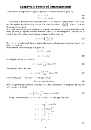
- 1. Langevin’s Theory of Paramagnetism The potential energy of the magnetic dipole in the external field is given by U = −→µB. −→ B (1) U = −µBB cos θ (2) According to Maxwell-Boltzmann statistics, at an absolute temperature T, the num- ber of magnetic dipoles having energy U is proportional to exp −U kBT . Where, kB is the Boltzmann’s constant. In a bulk material magnetic dipoles are oriented in random directions, therefore, con- tribution from all dipoles oriented between θ and θ + dθ with respect to the direction of applied filed −→ B per unit volume having energy U and is given by dn = Cexp −U kBT dΩ (3) Here, dΩ is the solid angle between two hollow cones of semi-vertex angles θ and θ + dθ, with c, a constant. By definition, the solid angle Ω is given by Ω = 2π(1 − cos θ) dΩ = 2π sin θdθ (4) from Eq.(3) and Eq.(4), we have dn = Cexp −U kBT 2π sin θdθ (5) Using Eq.(2) in (5), we have dn = Cexp µBB cos θ kBT 2π sin θdθ (6) substituting µBB kBT = x and 2πC = A in Eq.(6), we get dn = Aexp(x cos θ) sin θdθ (7) If we, integrate Eq.(7) between the limits (0, π), the total number of magnetic dipoles per unit volume is given by n = π 0 dn = π 0 Aexp(x cos θ) sin θdθ (8) Using the substitution cos θ = u, i.e. sin θdθ = −du in Eq.(8), we have n = −A −1 +1 exp(ux)du n = −A exp(ux) x −1 +1 n = −A e−x − e+x x n = A x (e+x − e−x ) (9) 1
- 2. n = 2A x sinh x (10) Now, the magnetization due to contribution of dn magnetic dipoles parallel to the field is given by the component µB cos θ. Whereas, the components perpendicular to the field cancels one another the, by symmetry. M = π 0 µB cos θdn (11) using Eq.(7) in Eq.(11), we have M = µBA π 0 cos θexp(x cos θ) sin θdθ Now use the substitution cos θ = u, i.e. sin θdθ = −du in Eq. 8, we have M = −µBA −1 +1 uexu du M = −µBA u ex u x − exu x du −1 +1 M = µBA u ex u x − exu x2 +1 −1 M = µBA ex u x u − 1 x +1 −1 M = µBA x ex 1 − 1 x − e−x −1 − 1 x M = µBA x ex + e−x − 1 x ex − e−x M = µBA x cos hx − sinh x x M = µBA x sinh x cothx − 1 x (12) Using Eq.(19) in Eq.(12), we obtain M = nµB coth x − 1 x M = nµBL(x) where L(x) = coth x − 1 x is known as Langevin’s function. For small values of x, the series expansion of L(x) reduce to L(x) = coth x − 1 x (13) L(x) ≈ x 3 Then the magnetization of the paramagnetic material is given by M = nµB x 3 µBB kBT = x (14) 2
- 3. M = nµ2 BB 3kBT (15) Also, we know that M is very small for pramagnetic materials. Hence the magnetic induction can be expressed as B = µ0(M + H) ≈ µ0H Then Eq.(15) takes the form M = nµ2 Bµ0H 3kBT (16) Hence, the magnetic susceptibility for a paramagnetic substances is given by χ = M H = nµ2 Bµ0 3kBT (17) In above Eq.(17), few important results can be pointed out from expression for the magnetic susceptibility • Magnetic susceptibility of the paramagnetic materials are positive. • Magnetic susceptibility varies inversely with temperature, i.e. χ ∝ 1 T (18) This is known as Curie’s law. • Magnetic susceptibility has no explicit dependence on B. n = 2A x sinh x (19) References [1] Solid state physics, Neil Ashcroft, Mermin, Brooks Cole, (1976). [2] www.google.com [3] www.arxiv.org 3