Assessing the relative importance of a variable in a heuristic model

1. International Journal of Statistics and Probability; Vol. 4, No. 2; 2015
ISSN 1927-7032 E-ISSN 1927-7040
Published by Canadian Center of Science and Education
123
Assessing Relative Importance Using RSP Scoring to Generate
Variable Importance Factor (VIF)
Daniel Koh1
1
School of Business, SIM University, Singapore
Correspondence: Daniel Koh, School of Business, SIM University, 461 Clementi Road, 599 491, Singapore. Tel:
65-6248-9746. E-mail: danielkoh005@unisim.edu.sg
Received: March 17, 2015 Accepted: April 8, 2015 Online Published: April 27, 2015
doi:10.5539/ijsp.v4n2p123 URL: http://dx.doi.org/10.5539/ijsp.v4n2p123
Abstract
Previous research has shown that the construction of VIF is challenging. Some researchers have sought to use
orderly contribution of R2
(coefficient of determination) as measurement for relative importance of variable in a
model, while others have sought the standardized parameter estimates b (beta) instead. These contributions have
been proven to be very valuable to the literature. However, there is a lack of study in combining key properties
of variable importance into one composite score. For example, an intuitive understanding of variable importance
is by scoring reliability, significance and power (RSP) of it in the model. Thereafter the RSP scores can be
aggregated together to form a composite score that reflects VIF. In this paper, the author seeks to prove the
usefulness of the DS methodology. DS stands for Driver‟s Score and is defined as the relative, practical
importance of a variable based on RSP scoring. An industry data was used to generate DS for practical example
in this paper. This DS is then translated into a 2x6 matrix where level of importance (LxI) is generated. The final
outcome of this paper is to discuss the use of RSP scoring methodology, theoretical and practical use of DS and
the possible future research that entails this paper. DS methodology is new to the existing literature.
Keywords: variable importance, decomposition of variances, RSP Scoring, multiple linear regression
1. Introduction
In recent history, much effort has been given to the study of variable importance factor (VIF). Researchers have
approached this topic in several manners: taking the increase of R2
– coefficient of determination - as the
usefulness of the regressors (Darlington, 1968), squared standardized coefficients and products of standardized
coefficients with marginal correlations (Hoffman, 1960; Hooker & Yule, 1906), LMG method of using sequential
sums of squares from the linear model (Lindeman, Merenda, & Gold, 1980), conditional variable importance for
Random Forest (Strobl, Boulesteix, Kneib, Augustin, & Zeileis, 2008), the averaging method of variance
decomposition (Kruskal, 1987; Chevan & Sutherland, 1991) and proportional marginal variance decomposition.
However, most of the studies are founded on one dimension. Several authors which include Ehrenberg (1990),
Stufken (1992), and Christensen (1992) have dismissed the usefulness and benefits of relative importance
measure. The premise of this dismissal was that the decomposition of coefficient of determination is too
simplistic and it is difficult to tease out relative importance among correlated variables which could potentially
“double count” in the model. In this paper, the focus is in the independent measurement of relative importance
and the discussion on teasing out interrelatedness between independent variables is deferred.
The decomposition of coefficient of determination becomes a powerful tool when complementary scorings are
given to improve accuracy in understanding relative importance of variables. Hence, this paper seeks to suggest
a new method to assess relative importance of variable by considering reliability, significance and power, to the
end that the final composite scores reflect the intuitive, practical understanding of relative importance better.
Reliability is defined here as the invert of the sum of residual errors between the predicted and actual values.
Significance is defined here as the heterogeneity of groupings with homogeneity in within-group distances or
maximized distances between predicted values with expected mean of dependent variable and minimized
distances between predicted values with actual values. Power is defined here as the positivity of the slope of the
estimates, with greater or steeper slope leading to greater power. The intention is to develop a score that not only
accounts for variance decomposition, but also practical meaningfulness and accuracy in utilizing a variable. It
also accounts for the goodness of a predictor by scoring the standardized parameter estimates of the variable in

2. www.ccsenet.org/ijsp International Journal of Statistics and Probability Vol. 4, No. 2; 2015
124
the model. The DS scoring methodology is new to our existing literature today.
2. Residual Errors as First Property
One aspect of a good predictor is its minimized residual error values, which then contribute to a strong
coefficient of determination, R2
. When residual errors are minimized, the chance of making mispredictions
becomes lesser, leading to greater reliability for the predictor. A practical example would be the reliability of age
in understanding income earnings. Between the independent variable age and gender, age is chosen to be the
better predictor for income earnings because gender may not contribute as much between-group residual errors
as compared to the sum of squares of model (SSM) for age. This is particularly true when a meritocratic society
promotes merit for work experiences, of which only age most likely correlates positively with it strongly,
regardless of gender type. Intuitively, the concept of reliability lies on the confidence of which one can get when
the model is put to test. The scores can be decomposed into respondent level, whereby each respondent is given
three scores for RSP, leading up to the final scoring of DS.
Hence, the first function of DS is the invert of residual errors, which is first expressed in the following
mathematical expression for multiple linear regression:
ŷ = 𝑎0 + 𝑎1 𝑥1 + 𝑎2 𝑥2 + … + 𝑎 𝑛 𝑥 𝑛 + 𝜀
(1)
where 𝑥 ∈ ℝ denotes the regressor, 𝑦̂ ∈ ℝ denotes the dependent variable, 𝑎 denotes the parameter
estimate and 𝜀 denotes the error term of the model.
A series of x is fitted into the model, generating a series of predicted values, ŷ. The residual for this model - 𝜁 -
is then expressed as the absolute difference between the actual values of the dependent variable which is denoted
by 𝑦 and the predicted values 𝑦̂.
𝜁 = |𝑦 − ŷ|
(2)
The residual is then inverted to form common directionality with two other functions of the RSP framework.
𝜌 =
1
𝜁
=
1
|𝑦 − ŷ|
(3)
The residual is then fitted onto the Gaussian‟s cumulative distribution function - Φ(𝜌) - , assuming that the
variable is independent and identically distributed (I.I.D) under the Normal distribution, 𝑋 ~ 𝑁(0,1):
Φ(𝜌) =
1
𝜍√2𝜋
∫ 𝑒−(𝜌−𝜇 𝜌)
2
/ 2𝜍 𝜌
2
𝑑𝜌
𝜌
min 𝜌
(4)
where 𝜌 denotes the inverse of residual error, 𝜇 𝜌 denotes the mean of the residual errors, 𝜍𝜌 denotes the
standard deviation of the residual error.
The first function of DS is improved when 𝜍2
𝜌 is decreased: reliability increases when data are less sparsely
distributed. This cumulative distribution function serves as a score for reliability on the observation or
respondent level. The use of the magnitude of 𝑅2
contributions to assess relative importance was similarly
proposed by Hoffman (1960) and later defended by Pratt (1987).
3. F-Ratios of the Residual Errors as Second Property
While the residual errors are expected to be minimized, the significance of the residual errors is expected to be
maximized. The motivation behind this property is to obtain scores that reflect variable‟s distinctiveness among
inter-groups through a study of variance ratio. For example, if a variable 𝜆 has unique and distinctive 𝜅
groupings in understanding income earning levels of a country, the F-Ratios due to 𝜆 should be greater as
compared to those that have more homogenous groupings.
The residual error in the first function is preferred over observations because the variance of residual errors
(variance study of residual errors) is expected to reflect distinctiveness between groups better if they are truly

3. www.ccsenet.org/ijsp International Journal of Statistics and Probability Vol. 4, No. 2; 2015
125
distinctive and unique than the observation values themselves. For example, when income is predicted using Age,
the error between 𝜅 groupings in 𝜆 should have distinctive noises. This “distinctive noises” should
characterize their identity as unique groupings in the model. This is true for variables that are categorical, which
will partition the data into kth groupings. Hence, the second function of DS has an inverse relationship with the
first function of DS.
The second function of DS - 𝜌 - is expressed in the following mathematical expression for a linear regression
model:
𝐹𝜌 =
𝑉𝑎𝑟𝑖𝑎𝑛𝑐𝑒𝑠 𝑑𝑢𝑒 𝑡𝑜 𝑀𝑜𝑑𝑒𝑙
𝑉𝑎𝑟𝑖𝑎𝑛𝑐𝑒𝑠 𝑑𝑢𝑒 𝑡𝑜 𝑅𝑒𝑠𝑖𝑑𝑢𝑎𝑙
(5)
𝐹𝜌 =
∑(𝑦̂ − 𝑦̅)2
(𝐾 − 1)
∑(𝑦 − 𝑦̂)2
(𝑁 − 𝐾)
(6)
𝐹𝜌 =
∑(𝑦̂ − 𝑦̅)2
∑(𝑦 − 𝑦̂)2
(
𝑁 − 𝐾
𝐾 − 1
*
(7)
where 𝐾 is the number of groupings, 𝑦̂ denotes predicted value of 𝑦, and 𝑦̅ denotes the average value of 𝑦,
N denotes the sample size.
The F-Ratios are then fitted into Fisher‟s CDF, which is the integral of the PDF of F-distribution, assuming that
the variables are independent and identically distributed (I.I.D) under the Fisher‟s distribution:
ΦFρ(Fρ,𝐾−1,𝑁−𝐾) = ∫
(
𝐾−1
𝑁−𝐾
)
𝐾−1
2
Fρ
K−1
2
− 1
(1+
K−1
N−K
Fρ)
−
N−1
2
[
*
1
2
(𝑁−𝐾)+!*
1
2
(𝐾−1)+!
*
1
2
(𝑁−𝐾)++*
1
2
(𝐾−1)+− 1
]
Fρ
0
(8)
Φϱ = 1 − ∫
(
𝐾 − 1
𝑁 − 𝐾
)
𝐾−1
2
Fρ
K−1
2
− 1
(1 +
K − 1
N − K
Fρ)
−
N−1
2
[
*
1
2
(𝑁 − 𝐾)+ ! *
1
2
(𝐾 − 1)+ !
*
1
2
(𝑁 − 𝐾)+ + *
1
2
(𝐾 − 1)+ − 1
]
Fρ
0
(9)
As F-ratio 𝐹𝜌 considers residual errors 𝜁, the Fisher‟s CDF ΦFρ(𝑥,𝐾−1,𝑁−𝐾) is reversed (1 − ΦFρ(Fρ,𝐾−1,𝑁−𝐾))
to generate significance score Φϱ, with greater residual errors leading to lower probability values.
This arrangement allows the decomposition of F-Ratios to the observation level, where each observation is
assigned an F-Ratio value. This cumulative distribution function which follows the Fisher‟s Distribution serves
as a score for Significance on the observation or respondent level.
Significance is an important property in DS. If income earnings are to be understood by gender and dwelling
type of individuals, the latter variable provides greater noises in residual error as the separating groups in the
factor create more „noises‟ than the variable gender. Or the noises between age and gender are significantly
different as the residual errors due to variable Age may contain more noises than the variable gender. If the

4. www.ccsenet.org/ijsp International Journal of Statistics and Probability Vol. 4, No. 2; 2015
126
distributions of errors among groupings are similar under the F-distribution, then the factor is less significant for
use as the factor exhibits homogeneity in variances across all groups. Hence, the significance of a variable relies
on the distinctiveness of errors between groups in factors, with homogeneity for within groups, or greater
distances from sample mean, with lower distances from the model.
4. Standardized Regression Coefficients as Third Property
The third and final function of DS is the standardized parameter estimate of the regressor. This is commonly
known as the slope of the curve. In a linear regression, the slope of the curve is observed by the parameter
estimates of the variable 𝑎 of the model. However, the use of unstandardized slope of the curve is not
appropriate when scales of different variables are different. Hence, the power of regressors – or „steepness‟ – is
then observed by the standardized parameter estimate 𝑏 of the model. This standardized estimate reduces the
metrical scale to a common vector across all regressors. It is expressed through the following mathematical
expression:
𝑦̇̂ = 𝑏̇1 𝜃1 + 𝑏̇2 𝜃2 + … + 𝑏̇ 𝑚 𝜃 𝑚 + 𝜀
(10)
𝑏 𝑚
̇ = 𝑏 𝑚 (
𝜍𝑥 𝑚
𝜍 𝑦
)
(11)
𝜃𝑖 denotes the standardized values of the predictor 𝑥, 𝑦̇̂ denotes the predicted response variable from
standardized predictors, 𝑏̇ 𝑚 denotes the standardized regression coefficient, 𝑏 𝑚 denotes the unstandardized
regression coefficient, 𝜍𝑥 denotes the standard deviation of the predictor and 𝜍 𝑦 denotes the standard deviation
of the response variable.
The absolute standardized regression coefficient – |𝑏 𝑚
̇ | – is then converted into a ratio out of the sum of all
absolute standardized coefficients, with 𝑛 number of parameters in a model:
𝜂 𝑗 =
|𝑏𝑗
̇ |
∑ |𝑏𝑗
̇ |𝑚
𝑗=1
(12)
where 𝑚 denotes the total number of parameter estimates in the model, 𝑏𝑗
̇ denotes the parameter estimate of
interest.
While relative importance measure considers reliability and significance, power is still necessary for the
understanding of relative importance of a variable in the model. When a powerful variable has low reliability and
significance, a low DS score is expected. If reliability and significance scores are high, but power score is low,
the DS still remains effective as the consideration that arises from the combined importance of reliability and
significance outweigh the consideration for power. Intuitively, power or standardized regression coefficient is not
the sole consideration of relative importance of a variable in the model but a combination of reliability,
significance and power.
5. Driver’s Score (DS)
Driver‟s Score (DS) is an aggregated score of three properties: reliability, significance and power. It reflects the
relative importance of a variable in the model practically. At the observation level, the Drivers‟ Score (𝛿) is the
geometric mean of these three properties. The mathematical expression is expressed as:
𝛿 = √(
1
𝜍√2𝜋
∫ 𝑒−(𝜌−𝜇 𝜌)
2
/ 2𝜍 𝜌
2
𝑑𝜌
𝜌
min 𝜌
. (1 − ∫
(
𝐾−1
𝑁−𝐾
)
𝐾−1
2
Fρ
K−1
2
− 1
(1+
K−1
N−K
Fρ)
−
N−1
2
[
*
1
2
(𝑁−𝐾)+!*
1
2
(𝐾−1)+!
*
1
2
(𝑁−𝐾)++*
1
2
(𝐾−1)+− 1
]
Fρ
0
) .
|𝑏 𝑗̇ |
∑ |𝑏 𝑗̇ |𝑚
𝑗=1
)
3
(13)
As observed in the DS equation, the DS methodology is the cube-root of the ratio of three products to the sum of

5. www.ccsenet.org/ijsp International Journal of Statistics and Probability Vol. 4, No. 2; 2015
127
all absolute standardized regression coefficient estimates. It is a function of Reliability (Gaussian‟s CDF which
has an exponential function), Significance (Fisher‟s CDF which has a function of the hypergeometric function
for 𝐹𝜌 by Beta function for 𝐹𝜌) and the absolute standardized regression coefficient of the variable of interest
and an inverse function of the sum of all absolute standardized regression coefficient estimates. The decrease in
other absolute standardized parameter estimates increases DS. This understanding has an important and practical
value: the variable of interest in which it is positioned with other variables is influenced by the mix of the model.
When DS is low, either two of the three properties or all properties are low, resulting to weaker drivers‟ influence.
When DS is high, either two of the three properties or all properties are high, resulting to stronger drivers‟
influence. DS is bounded by a lower limit and an upper limit of 0 and 1 respectively.
At the regressor level, the Drivers‟ Score (DS) is the arithmetic mean of all the geometric mean of all three
properties at the observation level:
𝛿̅ =
∑
( √(
1
𝜍√2𝜋
∫ 𝑒−(𝜌−𝜇 𝜌)
2
/ 2𝜍 𝜌
2
𝑑𝜌
𝜌
min 𝜌 .
(
1− ∫
(
𝐾−1
𝑁−𝐾
)
𝐾−1
2
Fρ
K−1
2
− 1
(1+
K−1
N−K
Fρ)
−
N−1
2
[
*
1
2
(𝑁−𝐾)+!*
1
2
(𝐾−1)+!
*
1
2
(𝑁−𝐾)++*
1
2
(𝐾−1)+− 1
]
Fρ
0
)
.|𝑏 𝑗̇ |
)
3
)
∑ |𝑏 𝑗̇ |𝑚
𝑗=1 .𝑛
(14)
When DS at the regressor level is low, relative influence on the dependent variable in the model is low. When DS
at the regressor level is high, relative influence on the dependent variable in the model is high. DS is bounded by
a lower limit and an upper limit of 0 and 1 respectively.
6. Weighted Drivers’ Score (wDS)
The weighted Drivers‟ Score (wDS) is a composite score of three properties (RSP), being weighted individually
by their importance in the DS framework. For example, the score for reliability (R) is far more important than
the score for significance (S) and power (P). Hence, the R score is given heavier weights than the rest. The wDS
- 𝛿 𝑤 - can be expressed mathematically by assigning power to the properties:
𝛿 𝑤 =
(
1
𝜍√2𝜋
∫ 𝑒−(𝜌−𝜇 𝜌)
2
/ 2𝜍 𝜌
2
𝑑𝜌
𝜌
min 𝜌 )
w1
.
(
1− ∫
(
𝐾−1
𝑁−𝐾
)
𝐾−1
2
Fρ
K−1
2
− 1
(1+
K−1
N−K
Fρ)
−
N−1
2
[
*
1
2
(𝑁−𝐾)+!*
1
2
(𝐾−1)+!
*
1
2
(𝑁−𝐾)++*
1
2
(𝐾−1)+− 1
]
Fρ
0
)
𝑤2
. |𝑏 𝑗̇ |
𝑤3
(∑ |𝑏 𝑗̇ |𝑚
𝑗=1 )
𝑤3 ,
𝑤1 + 𝑤2 + 𝑤3 = 1 (15)
At the regressor level, the weighted Drivers‟ Score which is relative importance of a variable in the model after
adding weights is the arithmetic mean of all three properties at the observation level:
𝛿̅ 𝑤 =
∑
(
(
1
𝜍√2𝜋
∫ 𝑒−(𝜌−𝜇 𝜌)
2
/ 2𝜍 𝜌
2
𝑑𝜌
𝜌
min 𝜌 )
w1
.
(
1− ∫
(
𝐾−1
𝑁−𝐾
)
𝐾−1
2
Fρ
K−1
2
− 1
(1+
K−1
N−K
Fρ)
−
N−1
2
[
*
1
2
(𝑁−𝐾)+!*
1
2
(𝐾−1)+!
*
1
2
(𝑁−𝐾)++*
1
2
(𝐾−1)+− 1
]
Fρ
0
)
𝑤2
. |𝑏 𝑗̇ |
𝑤3
)
(∑ |𝑏 𝑗̇ |𝑚
𝑗=1 )
𝑤3
.𝑛
(16)
7. Application of DS
Using data from a Multinational Corporation (MNC) that is based in Singapore (Note 1), the spread of DS of 4
predictors and its‟ response variable are:

6. www.ccsenet.org/ijsp International Journal of Statistics and Probability Vol. 4, No. 2; 2015
128
Figure 1. DS of v1 to v4 on dependent variable
Based on insights that were gathered from professionals in the industry, v1 has the greatest impact or driving
force in understanding the dependent variable. This impact or driving force is understood under the framework
of the RSP model. To garner reliable, significant and powerful dependent variable, extra care must be given to
v1.
As it is observed from the chart above (Figure 1), the relationship between DS and its dependent variable takes
on the inverse exponential function. This would explicitly highlight that the observations of RSP is often the
inverse of the dependent variable. The tendency to mispredict is higher when dependent variable or its set of
products gets too complex. In this area, the DS model has intuitively performed well.
Figure 2. Scatter-plots of DS with Dependent Variable
The plots in figure 2 show the area under the curve, which represents the magnitude of DS. V1 has the largest
area under the curve.
8. VIF and Its Decomposition
The relative importance of 𝑗 variable - 𝛿̅ - is the arithmetic mean of summation of all 𝛿 in 𝑗 variable:
0
10
20
30
40
50
0.000 0.100 0.200 0.300 0.400 0.500 0.600 0.700
Driver's Scores
Driver's Scores with Dependent Variable
v1 v2 v3 v4
0
10
20
30
40
50
0.00
0.09
0.12
0.14
0.18
0.20
0.22
0.25
0.28
0.32
0.35
0.39
0.43
0.48
0.54
Driver's Scores (DS)
v1 DS
0
10
20
30
40
50
0.00
0.21
0.20
0.27
0.31
0.39
0.32
0.29
0.27
0.26
0.47
0.32
0.26
0.35
0.40
0.31
Driver's Scores (DS)
v2 DS
0
10
20
30
40
50
0.00
0.09
0.08
0.05
0.12
0.07
0.22
0.21
0.12
0.11
0.16
0.14
0.18
0.12
0.23
0.14
Driver's Scores (DS)
v3 DS
0
10
20
30
40
50
0.03
0.20
0.15
0.23
0.30
0.47
0.38
0.37
0.29
0.29
0.18
0.28
0.14
0.20
0.10
0.14
Driver's Scores (DS)
v4 DS

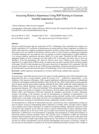
7. www.ccsenet.org/ijsp International Journal of Statistics and Probability Vol. 4, No. 2; 2015
129
𝛿𝑖,𝑗 = √Φ(𝜌 𝑖,𝑗). ΦFρ(Fρ,𝐾−1,𝑁−𝐾) . 𝜂 𝑗
3
(17)
𝛿̅𝑗 =
∑ 𝛿𝑖,𝑗
𝑛
𝑖=1
𝑛
(18)
Figure 3. VIF chart
As observed in the bar chart, the strongest relative importance of factor in the model is v1. This importance is
decomposed into its RSP properties, which is shown in the table below:
Table 1. Average RSP and DS Scores against Four Independent Variables
R S P DS
v1 0.5454 0.2148 0.3540 0.2867
v2 0.5481 0.3276 0.1830 0.2829
v3 0.5447 0.2067 0.0340 0.1363
v4 0.5364 0.1131 0.4290 0.2353
Mean 0.5437 0.2156 0.2500 0.2353
Note. The DS score is the geometric mean of all three RSP scores.
In this example, the use of the standardized parameter estimate – P - as the relative influence factor is misleading
as industry practitioners have clearly identified the importance of v1 rather than v4. This is also reflected in the
DS score. The other use of variance decomposition – R – is also misleading, as it identifies v2 as the factor that
has the strongest relative importance in the model instead of v1. The composite score of three properties clearly
show that variable importance does not solely rely on one aspect or dimension of importance considerations, but
three aspects: reliability, significance and power.
A 2x6 Variable Importance Matrix (VIM) describes the characteristics of DS. A low score is understood as a
score that is below 0.50. A high score is understood as a score that is above 0.50. For example, a mix of DS=0.90
(highest DS score in the model) and R=0.30 is characterized as the most important variable that has low
reliability. From the VIM table, this variable is known as an Unreliably Important variable.
Table 2. Variable Importance Matrix (VIM)
Less Important Most Important
Low Reliability Unreliably Trivial Unreliably Important
High Reliability Reliably Trivial Reliably Important
Low Significance Insignificantly Trivial
Insignificantly
Important
High Significance Significantly Trivial
Significantly
Important
Low Power Powerlessly Trivial
Powerlessly
Important
High Power Powerfully Trivial Powerfully Important
0.29 0.28
0.14
0.24
0
0.05
0.1
0.15
0.2
0.25
0.3
0.35
v1 v2 v3 v4
VIF based on DS scoring
VIF

8. www.ccsenet.org/ijsp International Journal of Statistics and Probability Vol. 4, No. 2; 2015
130
A classification by levels (CLASS) is used here:
If ALL RSP is low (i.e. 𝑅𝑆𝑃 < 0.50) ⇒ Level 4
If EITHER Two of RSP is low (i.e. 𝑅𝑃/𝑅𝑆/𝑆𝑃 < 0.50) ⇒ Level 3
If ONLY One of RSP is low (i.e. 𝑅/𝑆/𝑃 < 0.50) ⇒ Level 2
If NONE of RSP is low (i.e. 𝑅𝑆𝑃 ≥ 0.50) ⇒ Level 1
The CLASS logic is then combined with VIM to generate the final descriptive outcome of VIF for the variable
of interest. For example, v1 is classified as level 3 Importance (L3I) variable. However, DS can be improved if
the CLASS level improves from level 3 to level 1. Ideally, a good and strong driver for response variable is a
level 1 importance (L1I) variable. To achieve such a score, RSP scores that are below 0.50 should be given extra
attention. For example, v1 has high R score but low S and P scores. Hence, measures to create greater
distinctiveness and power could potentially improve the final DS score.
The benefit of this scoring methodology is 1) the flexibility to include categorical variables as a regressor, 2) the
ability to aggregate three important properties of variable from both the theoretical and practical aspects of
analytic, and 3) the simplicity at which an explanation could be given to laypeople.
Categorical variables are treated as dummy variables in the linear regression model and its‟ F-ratios are similarly
calculated by taking the sum of squared error due to model against the sum of squared error due to residual
errors. To assign power to the DS methodology, absolute standardized regression coefficients for each dummy
variable is assigned to each groupings in the factor. Hence, a metrical independent variable has one power
assignment in a factor while the categorical independent variable has multiple power assignments for different
groupings in a single factor.
Theoretically, so long as the variable is normally distributed and conforms to the chi-square distribution, the
usefulness of the DS methodology becomes essential for practical use. A single dimension of the DS
methodology may be taken to generate VIF measurement, but it does not represent the natural and intuitive
considerations of factor importance in practice. Practitioners often need a score that reflects reliability,
significance and power of the predictors and conclude the importance of it thereafter. DS helps to meet the needs
of those who wish to obtain a practical assessment of variable importance.
9. Limitations of DS
DS has several limitations. Firstly, DS takes the absolute standardized regression coefficients as a measurement
for power in a linear model. In cases where nonlinearity is observed, an alternative approach is needed to
substitute this third property of DS. Also, DS does not account for multi-dimensional explanation of variances in
a single vector space. This has implications when it comes to interrelatedness of predictors that could potentially
form interaction terms. When interaction terms are formed, the DS methodology is not able to tease out
interaction effects. Lastly, as categorical variables are converted into dummy variables in a model, the increase in
parameter estimates with constant set of sample size makes the model unstable. Hence, the DS methodology
becomes useful when only key factors that could potentially explain variances better are considered. These
limitations have an impact in practical use when the relationship between predictors and response variable
becomes too complex, resulting to multiple unknown „noises‟ within the model that could affect the whole DS
methodology. The use of DS should be jealously guarded by good and firm understanding of relationship
between variables and the intuitive approach in understanding practical relationships is essential in the DS
methodology.
10. Summary
Managers often ask what drivers or variables influence the outcome of success more significantly over the other
at the respondent level. For example, the main question that managers ask is the drivers which contribute to the
success of an event. Fundamentally, the drivers that contribute mostly to success of an event are obtained by the
correlation coefficient of the variables. However, this methodology falls apart when categorical variables are
used or the requirement to assess additional parameters is apparent. DS is designed to overcome this limitation
by decomposing the DS scores into its three properties – RSP. As the measurement for variable influence is seen
at the observation or respondent level, the aggregation of scores can finally add up to the variable influence
factor (VIF) measurement.
Cost-cutting measures that lead to improved profitability are also possible by using DS. Businesses can utilize
DS to determine which dimension or variable has the greatest importance and pitch marketing efforts on that
dimension with a targeted focus on respondents who have higher RSP scores. If the amount of sales leads is a

9. www.ccsenet.org/ijsp International Journal of Statistics and Probability Vol. 4, No. 2; 2015
131
stronger or more important factor in determining revenue and the higher RSP scores are found among the
entrepreneurs, then companies can focus their marketing effort on generating leads by targeting the entrepreneurs
first, then the others. Although it is fundamentally true that the outcome of revenue takes prerogative in
marketing effort, the precision of the outcome and the significance of it have a key role to play in understanding
variable importance. Targeted and focused marketing can generate income faster, which could then supplement
additional capital to target the rest of the populations using low-cost marketing efforts.
11. Future Research
Due to the limitation imposed by the DS methodology, more studies can be conducted to understand how
variance decomposition occurs in a multi-dimensional setting in a single vector space. Particularly, studies can
be conducted to examine independent variables that are correlated to each other and when these variables are
categorical, more can be done to examine interaction terms and how it decomposes to the RSP scorings. Finally,
more „real-world‟ data is needed to assess the DS methodology, particularly in RSP scorings. A survey of factor
importance can be distributed to industry practitioners to complement the findings of DS. The results from the
survey can validate the strength of RSP scoring methodology. While the RSP scoring and its DS methodology is
still at its conceptual stage, the use of it can bring many benefits to business practitioners and academic
researchers. In light of the possible use of DS, more industrial report can utilize this RSP scoring method to
generate analytic-based decision makings.
References
Chevan, A., & Sutherland, M. (1991). Hierarchical Partitioning. The American Statistician, 90-96.
http://dx.doi.org/10.2307/2684366
Christensen, R. (1992). Comment on "Hierarchical Partitioning," by A. Chevan and M. Sutherland. The
American Statistician , 74.
Darlington, R. (1968). Multiple Regression in Psychological Research and Practice. Psychological Bulletin ,
161-182. http://dx.doi.org/10.1037/h0025471
Ehrenberg, A. (1990). The Unimportance of Relative Importance. The American Statistician , 260.
Hoffman, P. (1960). The Paramophic Representation of Clinical Judgment. Psychological Bulletin , 116-131.
http://dx.doi.org/10.1037/h0047807
Hooker, R., & Yule, G. U. (1906). Note on Estimating the Relative Influence of Two Variables Upon a Third.
Journal of the Royal Statistical Society , 197-200. http://dx.doi.org/10.2307/2339552
Kruskal, W. (1987). Relative Importance by Averging Over Orderings. The American Statistician, 6-10.
Lindeman, R., Merenda, P., & Gold, R. (1980). Introduction to Bivariate and Multvariate Analysis. Glenview:
Scott, Foresman.
Pratt, J. W. (1987). Dividing the Indivisible: Using Simple Symmetry to Partition Variance Explained.
Proceedings of Second Tampere Conference in Statistics, eds. (pp. 245-260). Finland: T. Pukkila and S.
Puntamen.
Strobl, C., Boulesteix, A., Kneib, T., Augustin, T., & Zeileis, A. (2008). Conditional Variable Importance for
Random Forests. BMC Bioinformatics , 307. http://dx.doi.org/10.1186/1471-2105-9-307
Stufken, J. (1992). On Hierarchical Partitioning. The American Statistician , 70-71.
Note 1: With permission granted from the Multinational Corporation (MNC), under the condition of full
anonymity and non-disclosure.
Copyrights
Copyright for this article is retained by the author(s), with first publication rights granted to the journal.
This is an open-access article distributed under the terms and conditions of the Creative Commons Attribution
license (http://creativecommons.org/licenses/by/3.0/).