A cell consists of various molecules or substances.pdf
Prediction of Protein Solubility in Escherichia coli using Logistic regression
1. ARTICLE
Prediction of Protein Solubility in Escherichia coli
Using Logistic Regression
Armando A. Diaz, Emanuele Tomba, Reese Lennarson, Rex Richard,
Miguel J. Bagajewicz, Roger G. Harrison
School of Chemical, Biological and Materials Engineering, University of Oklahoma, 100 E.
Boyd St., Room T-335, Norman, Oklahoma 73019; telephone: 405-325-4367;
fax: 405-325-5813; e-mail: rharrison@ou.edu
Received 18 June 2009; revision received 18 August 2009; accepted 2 September 2009
Published online ? ? ? ? in Wiley InterScience (www.interscience.wiley.com). DOI 10.1002/bit.22537
ABSTRACT: In this article we present a new and more
accurate model for the prediction of the solubility of pro-
teins overexpressed in the bacterium Escherichia coli. The
model uses the statistical technique of logistic regression. To
build this model, 32 parameters that could potentially
correlate well with solubility were used. In addition, the
protein database was expanded compared to those used
previously. We tested several different implementations of
logistic regression with varied results. The best implementa-
tion, which is the one we report, exhibits excellent overall
prediction accuracies: 94% for the model and 87% by cross-
validation. For comparison, we also tested discriminant
analysis using the same parameters, and we obtained a less
accurate prediction (69% cross-validation accuracy for the
stepwise forward plus interactions model).
Biotechnol. Bioeng. 2009;9999: 1–10.
ß 2009 Wiley Periodicals, Inc.
KEYWORDS: protein solubility; logistic regression; discri-
minant analysis; inclusion bodies; Escherichia coli
Introduction
TheQ2
use of recombinant DNA technology to produce
proteins has been hindered by the formation of inclusion
bodies when overexpressed in Escherichia coli (Wilkinson
and Harrison, 1991). Inclusion bodies are dense, insoluble
protein aggregates that can be observed with the aid of an
electron microscope (Williams et al., 1982). The formation
of protein aggregates upon overexpression in E. coli is
problematic since the proteins from the aggregate must be
resolubilized and refolded, and then only a small fraction of the
initial protein is typically recovered (Singh and Panda, 2005).
To date, despite some efforts, highly consistent and
accurate prediction of protein solubility is not available.
Indeed, ab initio solubility prediction requires folding
prediction where interactions with the solvent and with
other proteins need to be considered. Some attempts to
obtain ab initio predictions of the folding of soluble proteins
(i.e., considering protein–water interactions) have been
made (Bradley et al., 2005; Klepeis and Floudas 1999; Klepeis
et al., 2003; Koskowski and Hartke, 2005; Scheraga, 1996).
Despite all these efforts, a tool for full and reliable ab initio
solubility predictions is not yet available. Jenkins (1998)
developed equations that describe the change of protein
solubility with changes in salt concentration, but these are
not ab initio predictions of protein solubility.
In the absence of good ab initio methods, and perhaps
helping their development, semi-empirical relationships
obtained from correlating parameters help predict protein
solubility with reasonable accuracy for proteins expressed in
E. coli at the normal growth temperature of 378C. For
example, discriminant analysis, a statistical modeling
technique, was first used by Wilkinson and Harrison
(1991) and later by Idicula-Thomas and Balaji (2005) and
has yielded some success.
Wilkinson and Harrison (1991) conducted a study using a
database of 81 proteins. Six parameters that were predicted
to help classify proteins as soluble or insoluble from
theoretical considerations were included in the model:
approximate charge average, cysteine fraction, proline
fraction, hydrophilicity index, total number of residues,
and turn-forming residue fraction. The prediction accuracy
was 81% for 27 soluble proteins and 91% for 54 insoluble
proteins. One potential problem with the database is that it
contained many proteins that were fusion partners, which
may have biased the model. Wilkinson and Harrison’s
discriminant model was later modified by Davis et al.
(1999), who found that the turn forming residues and the
approximate charge average were the only two parameters
that influenced the solubility of overexpressed proteins in E. coli.
Idicula-Thomas and Balaji (2005) performed discrimi-
nant analysis using a new set of parameters and a database of
170 proteins expressed in E. coli. In this model, the most
Correspondence to: R.G. Harrison
Additional Supporting Information may be found in the online version of this article.
ß 2009 Wiley Periodicals, Inc. Biotechnology and Bioengineering, Vol. 9999, No. 9999, 2009 1BIT-09-523.R1(22537)
2. important parameters were found to be the asparagine,
threonine, and tyrosine fraction, aliphatic index, and
dipeptide and tripeptide composition. When all the
variables were included in the classification function (except
dipeptide and tripeptide composition, which interfere with
the classification results), the cross-validation accuracy was
62% overall. In another study, Idicula-Thomas et al. (2006)
used a support vector machine learning algorithm to predict
the solubility of proteins expressed in E. coli. The parameters
used in the model were protein length, hydropathic index,
aliphatic index, instability index of the entire protein,
instability index of the N-terminus, net charge, single
residue fraction, and dipeptide fraction. The model was
developed on a training set of 128 proteins and then tested
for accuracy on a test set of 64 proteins. The overall accuracy
of prediction for the test set was 72%.
In the current study, logistic regression, which has not
been used previously for predicting protein solubility in
E. coli, is used. Compared to discriminant analysis, logistic
regression has the significant advantage that it does not
require normally distributed data. Also, an expanded
protein database and a more extensive set of parameters
than previously employed were used, with the parameters
being relatively straightforward to calculate. They are
outlined in Table I. In addition to all parameters of the
study from Wilkinson and Harrison (1991), 26 additional
parameters were added. Table I indicates which parameter
was used in previous models (Wilkinson and Harrison
denoted by W&H and Idicula-Thomas and Balaji, denoted
by IT&B). Another goal was to develop a model that, unlike
some others, can readily be used by others. Indeed, the
complete details of the models by Idicula-Thomas and Balaji
and by Idicula-Thomas et al., are not available.
We first discuss our protein database and the parameters
used to predict solubility. Next we review the models we
used, as well as the software. Finally we present our
methodology to establish the significance of parameters
followed by our results.
Methods
Protein Database
Literature searches were done to find studies where the
solubility or insolubility of a protein expressed in E. coli was
discovered, regardless of the focus of the article. Only
proteins expressed at 378C without fusion proteins or
chaperones were considered, and membrane proteins were
excluded (see Table S-I in the Supplementary Online
Material). Fusion proteins and the overexpression of
chaperones can make an insoluble protein soluble by
helping improve folding kinetics or changing its interactions
with solvent (Davis et al., 1999; Walter and Buchner, 2002).
This can give false positives, making an inherently insoluble
protein soluble. The temperature chosen is a common
temperature for much work done with E. coli, and it had to
be consistent because the temperature plays a factor in
protein folding in solubility. In determining the sequence of
each protein expressed, signal sequences that were not part
of the expressed protein were excluded due to their
hydrophobic nature. The signal sequence of a protein is a
short (5–60) stretch of amino acids, and these are found
in secretory proteins and transmembrane proteins. The
removal of these signal sequences does not affect the
prediction of protein solubility because at some point in
the folding pathway of these proteins, the signal sequence is
removed. The database contains a total of 160 insoluble
proteins and 52 soluble proteins. Of these 212 proteins, 52
were obtained from the dataset of Idicula-Thomas and Balaji
(2005).
The solubility or insolubility of the 212 proteins was
assigned as follows: Proteins that appeared almost entirely in
the inclusion body were classified as insoluble proteins.
Conversely if a significant amount of the protein appeared in
the soluble fraction, the protein was classified as soluble. The
significance of the expression of the protein in the soluble
fraction was determined by the SDS–PAGE when available.
Proteins that showed bands in the soluble lanes that were
more than faintly visible were identified as having a
Table I. Parameters used in this study.
Property Abbreviation Source
Molecular weight MW W&H
Cysteine fraction Cys W&H
Total number of hydrophobic residues Hydrophob. New
Largest number of contiguous
hydrophobic residues
Contig. hydrophob. New
Largest number of contiguous
hydrophilic residues
Contig. hydrophil. New
Aliphatic index Aliphat. IT&B
Proline fraction Pro W&H
a-Helix propensity a-Helix New
b-Sheet propensity b-Sheet New
Turn forming residue fraction Turn frac. W&H
a-Helix propensity/b-sheet propensity a-Helix/b-sheet New
Hydrophilicity index Hydrophil. W&H
Average pI pI New
Approximate charge average Charge avg. W&H
Alanine fraction Ala New
Arginine fraction Arg New
Asparagine fraction Asn IT&B
Aspartate fraction Asp New
Glutamate fraction Glu New
Glutamine fraction Gln New
Glycine fraction Gly New
Histidine fraction His New
Isoleucine fraction Iso New
Leucine fraction Leu New
Lysine fraction Lys New
Methionine fraction Met New
Phenylalanine fraction Phe New
Serine fraction Ser New
Threonine fraction Thr IT&B
Tyrosine fraction Tyr IT&B
Tryphophan fraction Tryp New
Valine fraction Val New
2 Biotechnology and Bioengineering, Vol. 9999, No. 9999, 2009
3. significant amount of protein in the soluble fraction. When
the SDS page was unavailable, the protein was classified
according to the qualitative information given that
described its expression in E. coli. The reason for assigning
the proteins this way was due to their overexpression in
E. coli. Overexpression causes conditions where even soluble
proteins will form inclusion bodies due to the cell becoming
overly crowded (Baneyx and Mujacic, 2004). Hence, when
proteins were expressed in significant amounts in both the
soluble fraction and inclusion bodies, it was assumed that
the inclusion bodies were formed due to overexpression and
that under normal expression the protein would fold
correctly and be soluble.
Parameters Used
Several parameters are used that potentially affect protein
folding and solubility. Protein folding describes the process
by which polypeptide interactions occur so that the shape of
the native protein is ultimately formed and is directly related
to solubility because an unfolded protein has more
hydrophobic amino acids exposed to the solvent (Murphy
and Tsai, 2006). Therefore, correct folding gives a protein a
much higher probability of being soluble in aqueous
solution because interactions between hydrophobic residue
and the solvent are minimized, when these residues are
within the protein interacting with other residues instead.
Before our data were analyzed with SAS, normalization of
the data was performed. In order to normalize the data, the
maximum value of each parameter was calculated (Table II).
The rationale for the use of each of the parameters is as
follows:
Molecular Weight
The molecular weight was added because it correlates better
with size than the number of residues. The molecular weight
of each protein was determined with aid of the pI/MW tool
from the Swiss Institute of Bioinformatics.
Cysteine Fraction
Disulfide linkages between cysteine residues are important
in protein folding because these bonds add stability to the
protein; if the wrong disulfide linkages are formed or cannot
form, the protein cannot find its native state and will
aggregate (Murphy and Tsai, 2006). For V-ATPase, an ATP-
dependent protein that is responsible for the translocation
of ions across membranes, it has been shown that the
formation of disulfide bridges is essential for the proper
folding and solubility of the protein (Thaker et al., 2007). An
important fact about E. coli is that when eukaryotic proteins
are expressed in E. coli, due to the reducing nature of E. coli’s
cytoplasm, these bonds cannot be formed (Wilkinson and
Harrison, 1991). The total number of cysteine (C) residues
found in a protein were added, and then this value was
divided by the total number of residues for a given protein.
Hydrophobicity-Related Parameters (Fraction of Total
Number of Hydrophobic Amino Acids and Fraction of
Largest Number of Contiguous Hydrophobic/Hydrophilic
Amino Acids)
The fraction of highest number of contiguous hydrophobic
and hydrophilic residues was used because a recent study as
a modification of a study by Dyson et al. (2004). Dyson et al.,
showed a pattern between the highest number of contiguous
hydrophobic residues and protein solubility: proteins with a
small number of contiguous hydrophobic residues were
found to be expressed in soluble form while those with a
high number were expressed as insoluble aggregates. This
was also addressed in an earlier study that also found that the
more concentrated hydrophobic residues were in a
sequence, the more likely the protein would form insoluble
aggregates (Schwartz et al., 2001). It has been shown that
long stretches of hydrophobic residues tend to be rejected
internally in proteins, meaning they are exposed to the
solvent (Dyson et al., 2004). These polar–nonpolar
Table II. Maximum value of parameters.
Parameter Maximum value
MW 577934
Cys 0.3279
Pro 0.1826
Turn frac. 0.4609
Contig. hydrophil. 0.2941
Charge avg. 0.3529
Hydrophil. 0.7435
Hydrophob. 0.7739
Contig. hydrophob. 0.122
Aliphat. 1.3281
a-Helix 1.1903
b-Sheet 0.4861
a-Helix/b-sheet 3.429
pI 12.01
Asn 0.1136
Thr 0.1311
Tyr 0.2632
Gly 0.2105
Ala 0.2
Val 0.1652
Iso 0.1263
Leu 0.1718
Met 0.0714
Lys 0.2105
Arg 0.2435
His 0.0949
Phe 0.0854
Tryp 0.0588
Ser 0.1311
Asp 0.1055
Glu 0.1301
Gln 0.1176
Diaz et al.: PredictionQ1
of Protein Solubility in E. coli 3
Biotechnology and Bioengineering
4. interactions will tend to make proteins aggregate. However,
it is noteworthy that some proteins accommodate long
stretches of hydrophobic residues in the folded core. For
instance, UDP N-acetylglucosamine enolpyruvyl transferase
successfully incorporates a 12-residue hydrophobic block in
its folded state (Dyson et al., 2004). These parameters were
calculated by finding the largest stretch of hydrophobic or
hydrophilic amino acid present in the protein, and then
these were divided by the total number of residues; amino
acids were classified hydrophobic or hydrophilic based in
the hydrophilicity index of all 20 amino acids (Hopp and
Woods, 1981).
Aliphatic Index
The aliphatic index was added following Idicula-Thomas
and Balaji (2005). This parameter is related to the mole
fraction of the amino acids alanine, valine, isoleucine, and
leucine. Proteins from thermophilic bacteria were found to
have an aliphatic index significantly higher than that of
ordinary proteins (Idicula-Thomas and Balaji, 2005), so it
can be used as a measure of thermal stability of proteins.
This parameter varies from the largest number of
contiguous hydrophobic amino acids because we are taking
the total number of aliphatic amino acids, whether they are
found contiguously or not, and only the aliphatic amino
acids (those whose R groups are hydrocarbons, e.g., methyl,
isopropyl, etc.) are taking into account. The aliphatic index
(AI) was calculated using the following equation (Idicula-
Thomas and Balaji, 2005):
AI ¼
ðnA þ 2:9nV þ 3:9ðnI þ nLÞÞ
ntot
(1)
where nA, nv, nI, nL, and ntot are the number of alanine,
valine, isoleucine, leucine, and total residues, respectively.
Secondary Structure-Related Properties (Proline
Fraction, a-Helix Propensity, b-Sheet Propensity,
Turn-Forming Residue Fraction, and a-Helix
Propensity/b-Sheet Propensity)
Forces that determine protein folding include hydrogen
bonding and nonbonded interactions (Dill, 1990; Klepeis
and Floudas, 1999) electrostatic interactions and formation
of disulfide bonds (Klepeis and Floudas, 1999; Murphy and
Tsai, 2006), torsional energy barriers across dihedral angles
and presence of proline residues in a protein (Klepeis and
Floudas, 1999). Hydrogen bonding interactions are involved
in alpha helices and beta sheet structures and other
interactions crucial to the formation of a protein in its
native state; however, these forces were thought not to be
dominant in protein folding (Dill, 1990). Studies have
shown that solvation contributions are significant forces in
stabilizing the native structure of proteins because of solvent
molecules that surround the protein in order to make a
hydration shell (Klepeis and Floudas, 1999). A recent study
showed that point mutations of residues that decrease alpha
helix propensity and increase beta sheet propensity in
apomyoglobin have been shown to cause protein aggrega-
tion (Vilasi et al., 2006). This indicated that alpha helices
may tend to favor solubility while beta sheets may tend to
favor aggregation. Another study supplied some support for
this hypothesis by showing that the regions of acylpho-
sphatase responsible for protein aggregation have high beta
sheet propensity (Chiti et al., 2002). Finally, studies of
secondary structure in inclusion bodies have shown high
content of beta sheets in inclusion with the beta sheet
content increasing with increasing temperature (Przybycien
et al., 1994). Since increased temperatures tend to cause
aggregation as well as cause beta sheet formation, it can be
inferred that the presence of beta sheets may favor
aggregation. The turn-forming residue fraction was found
by adding the total number of asparagines (N), aspartates
(D), glycines (G), serines (S), and prolines (P) and then
dividing the sum by the total number of residues in the
protein. These residues were chosen because they tend to be
found more frequently in turns (Chou and Fasman, 1978).
Alpha helical (Pace and Scholtz, 1998) and beta sheet
propensities (Street and Mayo, 1999) for each amino acid
were obtained from the literature. The average alpha helical
propensity for the protein was obtained by summing the
alpha helical propensities of all the amino acids in the
sequence and dividing by the total number of amino acids.
A similar procedure was used for beta sheet propensity.
Then, the former values were divided by the latter, in
order to create the parameter a-helix propensity/b-sheet
propensity.
Protein–Solvent Interaction Related Parameters
(Hydrophilicity Index, pI, and Approximate
Charge Average)
Electrostatic interactions are caused by the amino acid
residues which are charged at physiological pH (7.4), which
include positively charged lysine and arginine and negatively
charged aspartate and glutamate (Murphy and Tsai, 2006).
These interactions can help in protein folding and stability
by creating residue–solvent interactions at the protein
surface as well as residue–residue interactions within the
protein (Murphy and Tsai, 2006). The average hydro-
philicity index was found by summing the hydrophilicity
indices for all the amino acids and dividing by the total
number of amino acids (obtained from Hopp and Woods,
1981). The isoelectric point of each protein was determined
with aid of the pI/MW tool from the Swiss Institute of
Bioinformatics (ExPASy Proteomics Server, website address
http://ca.expasy.org). Finally, the charge average was found
by taking the absolute value of the sum of the difference
between the positively charged amino acids (K and R) and
the negatively charged residues (D and E) and dividing by
the total number of residues.
4 Biotechnology and Bioengineering, Vol. 9999, No. 9999, 2009
5. Alanine, Arginine, Asparagine, Aspartate, Glutamate,
Glutamine, Glycine, Histidine, Isoleucine, Leucine,
Lysine, Methionine, Phenylalanine, Serine, Threonine,
Tyrosine, Tryptophan, Valine Fractions
Threonine and tyrosine fractions were added because these
amino acids were found to affect the solubility of proteins in
E. coli in a previous discriminant analysis mode (Idicula-
Thomas and Balaji, 2005). Phenylalanine was found to
stabilize transmembrane domain interactions via GxxxG
motifs, which play a crucial role in the correct folding of
integral proteins (Unterreitmeier et al., 2007). The rest of the
amino acids were added to see if they could play some role
that was not yet foreseen. For each of these amino acids,
the fraction of each amino acid was obtained by dividing the
number of residues in the sequence by the total number of
residues.
Logistic Regression Model
Binomial logistic regression is a form of regression which is
used when the dependent variable is a dichotomy (it belongs
to one of two nonoverlapping sets) and the independent
variables are of any type (continuous or categorical, i.e.,
belonging to one or more categories without an intrinsic
ordering to the categories) (Hosmer and Lemeshow, 2000).
In our case, the dichotomy is soluble/insoluble and the
independent variables are the parameters. Thus, the goal is
to develop a model capable of separating data into these two
categories, depending on properties of proteins that could
affect positively or negatively the solubility. Thus, the linear
logistic regression model is the following:
log
pi
1 À pi
¼ a þ b1x1;i þ b2x2;i þ Á Á Á þ bnxn;i (2)
where pi is the probability for a datum to belong to one
group, n the number of characteristic parameters integrated
in the model, a an intercept constant, bj a coefficient for the
parameter j, and xj,i the value for the parameter j for datum i.
Thus, logistic regression provides the probability (pi) of a
certain protein to belong to one set or another. As stated
earlier, logistic regression does not require normally
distributed variables, it does not assume homoscedasticity
(random variables having the same finite variance) and, in
general, has less stringent requirements than ordinary least
square (OLS) regression. The parameters a and bj,i are
calculated using the maximum likelihood method and a set
of given proteins whose solubility and parameters are
known. When applied to proteins that are not part of the
database used to build the model, the corresponding data
plugged in Equation (1) produces a value of pi, the
probability of the protein of being soluble or not. This
probability value is then compared to the cut-off set in the
SPSS software. The cut-off, for this model, was generally set
at pi ¼ 0.5 in SPSS. If the pi-value of the protein was less than
0.5, then the protein belonged to one group. If the P-value
was larger than 0.5, then the protein belonged to the other
group. Cut-off values down to 0.2 were also used for one
case.
Discriminant Analysis Models
Discriminant analysis is a statistical test technique that
separates two distinct groups by means of a function called
the discriminant function. This function maximizes the
ratio of between class variance and minimizes the ratio of
within class variance. As in the case of logistic regression,
proteins are classified into two groups (soluble and
insoluble) and the same group of parameters are used.
For a two-group system the linear discriminant function is
of the following form:
CVi ¼ a þ l1x1;i þ l2x2;i þ Á Á Á þ lnxn;i (3)
where CVi is the canonical variable for a specific datum, xj,i
the value of parameter j for a specific datum i, a a constant,
lj the coefficient for parameter j, and n the number of
characteristic parameters in the model. Although the
constant a is in general not needed, it is reported back in
programs like SPSS, so we left it for completeness.
The coefficients for each parameter (lj) and the value of a
are determined by maximizing the ability to distinguish data
between groups. Discriminant analysis also provides a
reference value for the canonical variables, namely CVÃ
,
which is used later for classification. At the end, the
parameters with the higher coefficients are the ones that are
largely responsible for the discrimination between the two
groups. When applied to proteins that are not part of the
database used to build the model, the corresponding data
produces a value of CVi, which is compared to CVÃ
. The
protein is then determined to be soluble or insoluble
depending on whether CVi is larger or smaller than CVÃ
.
Models With Interaction Among Parameters
In any model, an interaction between two variables implies
that the effect of one of the variables is not constant over
the levels of the other (Hosmer and Lemeshow, 2000). We
created interaction variables by taking the arithmetic
product of pairs of original parameters (main effect
variables or two-way interactions).
In this case, the model equation used for logistic
regression is
log
pi
1 À pi
¼ a þ
Xn
j¼1
bjxj;i þ
Xn
k¼1
Xn
j¼1;j6¼k
gk;jxj;ixk;i (4)
where n is the number of significant parameters, and j and k
represent the parameters. Interactions between the same
parameter were not included, so j is not equal to k. For
Diaz et al.: PredictionQ1
of Protein Solubility in E. coli 5
Biotechnology and Bioengineering
6. discriminant analysis, the model equation is
CVi ¼ a þ
Xn
j¼1
ljxj;i þ
Xn
k¼1
Xn
j¼1;j6¼k
mk;jxj;ixk;i (5)
Software and Websites Used
SPSS 15.0 for Windows was utilized to build and evaluate all
the logistic regression and discriminant analysis models,
in particular to obtain models coefficients and classification
tables. Leave-one-out cross-validation for logistic regression
was programmed in Matlab 7.4.0, using the output from
SPSSQ3
. Microsoft Excel was also used extensively in creating
the protein database and calculating protein parameters.
The National Center of Biotechnology Information Data-
base (NCBI) was consulted to obtain amino acid sequences.
Methods for Establishing Significance
Full datasets were imported to SPSS from the database and
evaluated using the LOGISTIC REGRESSION or DISCRI-
MINANT ANALYSIS procedure. In order to classify our
proteins, we utilized both linear and quadratic models, using
different approaches to the construction of the models. For
each method, SPSS generates the output with all coefficients
estimates and with the significance of every variable. The
significance is the probability value of the null hypothesis
for each parameter. The null hypothesis is that a parameter
does not affect the distinction between groups, so high
probability values indicate that parameters have little
significance on classification. In addition, we tested two
different approaches to obtain model coefficients: Step
Backward and Step Forward. The intention here is to remove
from the model those parameters that are not significant,
that is, their contribution is negligible. We also explored
interactions between parameters. We describe these
approaches next:
Stepwise Forward
The stepwise forward method builds the model by adding a
variable one at a time on the basis of its significance. The
significance of each parameter is determined first by using
the likelihood ratio or Wald’s test for logistic regression
model and the F-value or Wilks’ lambda for discriminant
analysis. Then the parameter with the smallest significance is
chosen. If the parameter’s significance is smaller than
the threshold (0.1 in our case), the parameter is chosen to be
part of the model, otherwise it is disregarded and the
parameter with the next lowest significance is chosen. In
the next step, the procedure is repeated by calculating the
significance of the remaining parameters, when used
together with the already chosen parameters. Then, the
parameter with a smaller significance than the threshold of
0.1 is chosen. If no parameter can be added, then the
program stops; otherwise, this procedure continues until no
new parameter can be added. After adding a new parameter
to the model, the significance of all parameters chosen to be
in the model is calculated. If any parameter has a significance
that is above 0.1, our threshold, then the parameter is taken
out of the model.
Stepwise Backward
The procedure starts from the all-independent parameters
model. At each step, the variable with the largest probability
value of not affecting the distinction between soluble and
insoluble proteins, that is, the least significant, is removed,
provided that this value is larger than a default probability
value for a variable removal (we set it at 0.10). The loop
continues until all the remaining variable’s significance in
the model are under the default probability value (0.10 in
our case).
Cross-Validation
Cross-validation is a method used in statistics to test how
well the logit function or discriminant function will classify
future data. It consists of four steps:
I. Temporarily remove ith
entry from database.
II. Obtain the logit or discriminant function with N À 1
entries, where N is the number of proteins.
III. Re-introduce ith
entry and run the logistic regression or
discriminant analysis again to obtain the classification
accuracy.
IV. An average of the classification accuracy obtained from
all N runs is then reported.
The coefficients of the model that are reported are the
ones obtained using all N proteins.
Results
The stepwise backward model gave poor results for soluble
proteins, with cross-validation accuracy of less than 10%.
Thus, we abandoned this option and concentrated on the
step forward one. In the case of considering interactions,
because the number of variables is larger than the number of
observations (528 variables against 212 observations), the
only method we could use when interactions are present is
the stepwise forward method.
The results of cross-validation for logistic regression and
discriminant analysis of models with and without interac-
tions using step forward significance methods are given in
Tables III and IV. It is clear that logistic regression gives
much better results.
The parameters that were found to be the most significant
for the model with interactions and stepwise forward
6 Biotechnology and Bioengineering, Vol. 9999, No. 9999, 2009
7. significance determination are shown in Table V; also shown
are the values of a, the constant, the standard error (SE), the
Wald statistic, the degrees of freedom (df), and the
significance (P) level. Tables VI and VII show the results
of the classification accuracies of the stepwise forward
models for logistic regression and discriminant analysis with
and without interactions. As expected, these accuracies
are larger than those obtained in the validation step. The
overall classification accuracy of the stepwise forward plus
interaction model in logistic regression was 93.9%, and the
overall cross-validation classification accuracy was 87.3%.
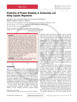
The classification accuracy of the stepwise forward with
interactions logistic regression model was found to vary
greatly with the predicted probability of solubility, as shown
in Figure 1. We also added how many proteins were
falling in each range. As one would expect, the region
close to the cut-off probability (0.5 in our case) is the one
exhibiting the lowest accuracy. However, the number of
proteins falling in this range is very small. In fact, most of the
proteins are in the 0–5% range and in the 95–100% range,
which speaks well about the power of the logistic regression.
The figure is useful, because once one applies the correlation
and obtains a value of pi for a new protein one can also
associate certain accuracy to the prediction. For example, if a
new protein exhibits a value of P ¼ 35%, then one could say
that the protein is insoluble with a 65% probability. The
accuracy of such a statement would be very high (close to
100%).
The cut-off for logistic regression was also moved from
0.5 to 0.2, and this improved the classification accuracy of
soluble proteins even though the overall classification
decreased due to the lower classification accuracy of
insoluble proteins (see Table VIII). The best model overall
was obtained from using a cut-off of 0.5.
There were three other models that were used, but no
success was achieved. These were the all squared rooted
parameters, the all squared parameters, and the all squared
parameters plus squared interactions models. Both
squared models were obtained from the generalized linear
model, and this was attempted due to its popularity when
binary data (like in our case where there is a binary option
for soluble and insoluble) is present (McCullagh and Nelder,
1989). When the data are squared, the results showed that
the classification is quasi-complete, a problem encountered
when some values of the target variable (either soluble or
insoluble) overlap or are tied at a single or only a few values
of the predictor variable (in this case, the predictor variables
are the parameters).
Table IV. Cross-validation accuracies for discriminant analysis models.
Model
Average accuracy of prediction
Soluble Insoluble Overall
Stepwise forward without interactions 59.4 59.6 59.6
Stepwise forward with interactions 57.7 73.1 69.3
Table V. Logistic regression modeling results for the logistic regression
model with interactions.
b SE Wald df Sig. Exp(b)
pI Â MW 96.236 34.632 7.722 1 0.005 6.23E þ 041
MW Â Ser À118.027 41.478 8.097 1 0.004 0.000
Asn  Pro 64.292 17.574 13.384 1 0.000 8E þ 27
Charge avg. Â Thr À323.429 67.921 22.675 1 0.000 0.000
Charge avg. Â Ser 204.869 43.594 22.085 1 0.000 9.41E þ 088
Hydrophil. Â Leu 74.534 21.105 12.471 1 0.000 2E þ 032
Hydrophil. Â Met À66.255 20.054 10.916 1 0.001 0.000
Hydrophil. Â His À209.900 52.569 15.943 1 0.000 0.000
Hydrophil. Â Phe 101.938 28.242 13.028 1 0.000 1.866E þ 04
Aliphat. Â Glu 66.886 17.413 14.754 1 0.000 1E þ 29
pI Â Gln 70.974 17.649 16.172 1 0.000 7E þ 30
Asn  His 16.590 9.822 2.853 1 0.091 2E þ 7
Iso  Thr 58.669 16.118 13.249 1 0.000 3E þ 25
Ala  Phe 52.071 12.938 16.198 1 0.000 4E þ 22
Ala  Tryp 38.762 13.436 8.322 1 0.004 7E þ 16
Met  Val À71.483 21.224 11.344 1 0.001 0.000
Asp  Val 64.379 14.918 18.624 1 0.000 9E þ 27
Glu  Iso À61.875 18.389 11.322 1 0.001 0.000
Asp  Met 88.432 21.132 17.512 1 0.000 3E þ 38
Arg  Lys À51.042 24.148 4.468 1 0.035 0.000
Arg  Phe À41.556 15.146 7.528 1 0.006 0.000
Ser  Tryp 59.630 16.544 12.992 1 0.000 8E þ 25
Asp  Tryp À88.447 23.019 14.763 1 0.000 0.000
Asp  Gln À92.899 23.268 15.941 1 0.000 0.000
Constant a À46.532 10.650 19.091 1 0.000 0.000
Table III. Cross-validation accuracies for logistic regression models.
Model
Average accuracy of prediction
Soluble Insoluble Overall
Stepwise forward without interactions 3.9 96.3 73.6
Stepwise forward with interactions 73.1 91.9 87.3
Table VI. Classification accuracies for the logistic regression model.
Model
Average accuracy of prediction
Soluble Insoluble Overall
Stepwise forward without interactions 9.6 97.5 75.9
Stepwise forward with interactions 86.5 96.3 93.9
Table VII. Classification accuracies for the discriminant analysis model.
Model
Average accuracy of prediction
Soluble Insoluble Overall
Stepwise forward without interactions 61.5 59.4 59.9
Stepwise forward with interactions 57.7 75 70.8
Diaz et al.: PredictionQ1
of Protein Solubility in E. coli 7
Biotechnology and Bioengineering
8. Discussion
Based on the results of this study, logistic regression is better
than discriminant analysis for predicting the solubility of
proteins expressed in E. coli. This is not surprising because
logistic regression is a more robust method (data do not to
be normally distributed and several other restriction for
DA do not hold). An important finding for the logistic
regression modeling is that only parameters that involve
interactions are significant in the model (see Table V). This
is really not a surprising result, since the correct folding of a
protein is an interactive process. The parameters besides the
fractions of individual amino acids that were found to
be significant in the best logistic regression model (stepwise
forward þ interactions) along with another parameter were
average pI, molecular weight, charge average, hydrophilicity
index, and aliphatic index (see Table V). The hydrophilicity
index appeared four times with another parameter, and
average pI, molecular weight, and charge average each
appeared two times with another parameter. The average pI
is related to the charge average, since the difference in the pI
of a protein and the pH in the cell is an indication of the
degree of charge on the protein. Hydrophilicity index and
charge average are two of the parameters that Wilkinson and
Harrison (1991) found to influence the solubility of proteins
expressed in E. coli. Idicula-Thomas and Balaji (2005) found
aliphatic index to be important in their model of protein
solubility in E. coli. Of the amino acids that Idicula-Thomas
and Balaji found to be significant, the asparagine fraction
and threonine fraction appeared two times with another
parameter in the logistic regression model using the stepwise
forward þ interactions method (Table V). The amino acid
that appears the most times with another parameter is
aspartic acid (four times), which is also a contributor to the
Figure 1. Classification accuracy of the stepwise forward plus interaction model as a function of the solubility prediction range. The numbers on the top of each bar represent
the number of proteins in that range.
Table VIII. Stepwise forward plus interaction model at different cut-offs.
Model: stepwise
forward þ interactions
Classification accuracy
Soluble Insoluble Overall
Cut-off ¼ 0.5 86.5 96.3 93.9
Cut-off ¼ 0.4 90.4 94.4 93.4
Cut-off ¼ 0.3 90.4 93.1 92.5
Cut-off ¼ 0.2 92.3 90.6 91.0
8 Biotechnology and Bioengineering, Vol. 9999, No. 9999, 2009
9. charge average; this further emphasizes the well-known role
of charge in the prediction of protein solubility.
We used a much larger dataset of proteins (212) for our
logistic regression model than Wilkinson and Harrison used
in their model (81). Also, no fusion proteins were used in
our model, while in Wilkinson and Harrison’s model, 41%
of the proteins were fusions. Applying Wilkinson and
Harrison’s model to our dataset, we found high classifica-
tion accuracy for insoluble proteins (93%) but a very low
accuracy for soluble proteins (4%). This same trend was also
found when applying the Davis et al. (2000Q4
) model to our
data. Therefore, it appears that the use of a relatively small
number of proteins and a high percentage of fusion proteins
skewed the Harrison–Wilkinson and Davis et al. discrimi-
nant analysis models.
The results indicate that while the classification accuracy
of the stepwise forward with interactions model is very good
for the set of soluble protein (86%), it is even better for the
set of insoluble proteins (96%). Two possible reasons for this
difference are the number of proteins in each group and
the parameters used in the model. While a reasonably
large set of proteins was used for the set of soluble proteins
(52), it was considerably smaller than the set of insoluble
proteins (160). Using a larger set of soluble proteins may
lead to an improvement in the prediction accuracy for this
set. Also, for the soluble proteins there may be additional
parameters that could be added to the model to improve
the prediction accuracy. The model may not be reflecting
the complexity of the process to produce a protein in soluble
form.
The model we have developed can be used to make
experimental work involving recombinant protein expres-
sion more efficient. Proteins with a high-predicted prob-
ability of solubility can be expressed in soluble form at 378C
with a high-degree of confidence, without the need for
expression using a fusion to promote solubility. Proteins
with intermediate predicted probability of solubility (50–
70%) are possibly soluble when expressed at temperatures
lower than 378C, which has been found to increase solubility
(Schein and Noteborn, 1988). Proteins with a predicted
solubility of less than 50% will probably require other means
to facilitate solubility, for example, by using a fusion partner
known to increase solubility, such as maltose binding
protein or NusA protein (Douette et al., 2005).
Electronic Supplementary Material
Electronic supplementary material includes the accession
number of the protein used in the models (Table S-I) and
the literature references used to collect proteins for the
database.
We thank undergraduate students Dolores Gutierrez-Cacciabue,
Nathan Liles, and Zehra Tosun for their help in developing the
protein database. We are grateful to Professor Jorge Mendoza
at the University of Oklahoma for his valuable suggestions and
assistance.
References
Baneyx F, Mujacic M. 2004. Recombinant protein folding and misfolding in
Escherichia coli. Nat Biotechnol 22:1399–1408.
Bradley P, Misura KM, Baker D. 2005. Toward high-resolution de novo
structure prediction for small proteins. Science 309:1868–1871.
Chiti F, Taddei N, Baroni F, Capanni C, Stefani M, Ramponi G, Dobson
CM. 2002. Kinetic partitioning of protein folding and aggregation. Nat
Struct Biol 9:137–143.
Chou PY, Fasman GD. 1978. Prediction of the secondary structure of
proteins from their amino acid sequence. Adv Enzymol Relat Areas Mol
Biol 47:45–148.
Davis GD, Elisee C, Newham DM, Harrison RG. 1999. New fusion protein
systems designed to give soluble expression in Escherichia coli. Bio-
technol Bioeng 65:382–388.
Dill KA. 1990. Dominant forces in protein folding. Biochemistry 29:7133–
7155.
Douette P, Navet R, Gerkens P, Galleni M, Levy D, Sluse FE. 2005.
Escherichia coli fusion carrier proteins act as solubilizing agents for
recombinant uncoupling protein 1 through interactions with GroEL.
Biochem Biophys Res Commun 333:686–693.
Dyson MR, Shadbolt SP, Vincent KJ, Perera RL, McCafferty J. 2004.
Production of soluble mammalian proteins in Escherichia coli: Identi-
fication of protein features that correlate with successful expression.
BMC Biotechnol 4:32–49.
Hopp TP, Woods KR. 1981. Prediction of protein antigenic determinants
from amino acid sequences. Proc Natl Acad Sci USA 78:3824–3828.
Hosmer DW, Lemeshow S. 2000. Applied logistic regression. New York:
Wiley, xii, 373 p.
Idicula-Thomas S, Balaji PV. 2005. Understanding the relationship between
the primary structure of proteins and its propensity to be soluble on
overexpression in Escherichia coli. Protein Sci 14:582–592.
Idicula-Thomas S, Kulkarni AJ, Kulkarni BD, Jayaraman VK, Balaji PV.
2006. A support vector machine-based method for predicting the
propensity of a protein to be soluble or to form inclusion body on
overexpression in Escherichia coli. Bioinformatics 22:278–284.
Jenkins WT. 1998. Three solutions of the protein solubility problem.
Protein Sci 7:376–382.
Klepeis JL, Floudas CA. 1999. Polymers, biopolymers, and complex sys-
tems—Free energy calculations for peptides via deterministic global
optimization. J Chem Phys 110:7491–7512.
Klepeis JL, Pieja MJ, Floudas CA. 2003. Biophysical theory and modeling—
Hybrid global optimization algorithms for protein structure prediction:
Alternating hybrids. Biophys J 84:869–882.
Koskowski F, Hartke B. 2005. Towards protein folding with evolutionary
techniques. J Comput Chem 26:1169–1179.
McCullagh P, Nelder JA. 1989. Generalized linear models. London; New
York: Chapman and Hall, xix, 511 p.
Murphy RM, Tsai AM. 2006. Misbehaving proteins: Protein (mis)folding,
aggregation, and stability. New York: Springer, viii, 353 p.
Pace CN, Scholtz JM. 1998. A helix propensity scale based on experimental
studies of peptides and proteins. Biophys J 75:422–427.
Przybycien TM, Dunn JP, Valax P, Georgiou G. 1994. Secondary structure
characterization of beta-lactamase inclusion bodies. Protein Eng 7:131–
136.
Schein CH, Noteborn MHM. 1988. Formation of soluble recombinant
proteins in Escherichia coli is favored by lower growth temperature.
Biotechnology (NY) 6:291–294.
Scheraga HA. 1996. Recent developments in the theory of protein folding:
Searching for the global energy minimum. Biophys Chem 59:329–339.
Schwartz R, Istrail S, King J. 2001. Frequencies of amino acid strings in
globular protein sequences indicate suppression of blocks of consecu-
tive hydrophobic residues. Protein Sci 10:1023–1031.
Singh SM, Panda AK. 2005. Solubilization and refolding of bacterial
inclusion body proteins. J Biosci Bioeng 99:303–310.
Street AG, Mayo SL. 1999. Intrinsic beta-sheet propensities result from van
der Waals interactions between side chains and the local backbone.
Proc Natl Acad Sci USA 96:9074–9076.
Diaz et al.: PredictionQ1
of Protein Solubility in E. coli 9
Biotechnology and Bioengineering
10. Thaker YR, Roessle M, Gruber G. 2007. The boxing glove shape of subunit d
of the yeast V-ATPase in solution and the importance of disulfide
formation for folding of this protein. J Bioenerg Biomembr 39:275–
289.
Unterreitmeier S, Fuchs A, Schaffler T, Heym RG, Frishman D, Langosch D.
2007. Phenylalanine promotes interaction of transmembrane domains
via GxxxG motifs. J Mol Biol 374:705–718.
Vilasi S, Dosi R, Iannuzzi C, Malmo C, Parente A, Irace G, Sirangelo I. 2006.
Kinetics of amyloid aggregation of mammal apomyoglobins and
correlation with their amino acid sequences. FEBS Lett 580:1681–
1684.
Walter S, Buchner J. 2002. Molecular chaperones—Cellular machines for
protein folding. Angew Chem Int Ed Engl 41:1098–1113.
Wilkinson DL, Harrison RG. 1991. Predicting the solubility of recombinant
proteins in Escherichia coli. Biotechnology (NY) 9:443–448.
Williams DC, Van Frank RM, Muth WL, Burnett JP. 1982. Cytoplasmic
inclusion bodies in Escherichia coli producing biosynthetic human
insulin proteins. Science 215:687–689.
Q1: Author: Please check the suitability of the short title on the odd-numbered pages. It has been formatted to fit the journal’s 45-character
(including spaces) limit.
Q2: Author: Please check the section heading suggested.
Q3: Author: Please provide complete location.
Q4: Author: Please add in the reference list.
10 Biotechnology and Bioengineering, Vol. 9999, No. 9999, 2009
11. 111 RIVER STREET, HOBOKEN, NJ 07030
***IMMEDIATE RESPONSE REQUIRED***
Your article will be published online via Wiley's EarlyView® service (www.interscience.wiley.com) shortly after receipt of
corrections. EarlyView® is Wiley's online publication of individual articles in full text HTML and/or pdf format before release of
the compiled print issue of the journal. Articles posted online in EarlyView® are peer-reviewed, copyedited, author corrected,
and fully citable via the article DOI (for further information, visit www.doi.org). EarlyView® means you benefit from the best of
two worlds--fast online availability as well as traditional, issue-based archiving.
Please follow these instructions to avoid delay of publication.
READ PROOFS CAREFULLY
• This will be your only chance to review these proofs. Please note that once your corrected article is posted
online, it is considered legally published, and cannot be removed from the Web site for further corrections.
• Please note that the volume and page numbers shown on the proofs are for position only.
ANSWER ALL QUERIES ON PROOFS (Queries for you to answer are attached as the last page of your proof.)
• Mark all corrections directly on the proofs. Note that excessive author alterations may ultimately result in delay of
publication and extra costs may be charged to you.
CHECK FIGURES AND TABLES CAREFULLY
• Check size, numbering, and orientation of figures.
• All images in the PDF are downsampled (reduced to lower resolution and file size) to facilitate Internet delivery.
These images will appear at higher resolution and sharpness in the printed article.
• Review figure legends to ensure that they are complete.
• Check all tables. Review layout, title, and footnotes.
COMPLETE REPRINT ORDER FORM
• Fill out the attached reprint order form. It is important to return the form even if you are not ordering reprints. You
may, if you wish, pay for the reprints with a credit card. Reprints will be mailed only after your article appears in
print. This is the most opportune time to order reprints. If you wait until after your article comes off press, the
reprints will be considerably more expensive.
RETURN PROOFS
REPRINT ORDER FORM
CTA (If you have not already signed one)
RETURN IMMEDIATELY AS YOUR ARTICLE WILL BE POSTED ONLINE SHORTLY AFTER RECEIPT;
FAX PROOFS TO 201-748-7670
QUESTIONS? Production Editor
E-mail:bitprod@wiley.com
Refer to journal acronym and article production number
(i.e., BIT 00-001 for Biotechnology and Bioengineering ms 00-001).
12. Color figures were included with the final manuscript files that we received for your article. Because of the high cost of
color printing, we can only print figures in color if authors cover the expense.
Please indicate if you would like your figures to be printed in color or black and white. Color images will be reproduced
online in Wiley InterScience at no charge, whether or not you opt for color printing.
You will be invoiced for color charges once the article has been published in print.
Failure to return this form with your article proofs will delay the publication of your article.
JOURNAL
BIOTECHNOLOGY AND BIOENGINEERING
MS. NO.
NO. OF
COLOR
PAGES
TITLE OF
MANUSCRIPT
AUTHOR(S)
No. Color Pages Color Charges No. Color Pages Color Charges No. Color Pages Color Charges
1 500 5 2500 9 4500
2 1000 6 3000 10 5000
3 1500 7 3500 11 5500
4 2000 8 4000 12 6000
***Please contact the Production Editor for a quote if you have more than 12 pages of color***
Please print my figures in black and white
Please print my figures in color
Please print the following figures in color:
BILLING
ADDRESS:
14. D. CONTRIBUTIONS OWNED BY EMPLOYER
1. If the Contribution was written by the Contributor in the course of the
Contributor’s employment (as a “work-made-for-hire” in the course of
employment), the Contribution is owned by the company/employer which
must sign this Agreement (in addition to the Contributor’s signature) in the
space provided below. In such case, the company/employer hereby assigns to
Wiley-Blackwell, during the full term of copyright, all copyright in and to the
Contribution for the full term of copyright throughout the world as specified in
paragraph A above.
2. In addition to the rights specified as retained in paragraph B above and the
rights granted back to the Contributor pursuant to paragraph C above, Wiley-
Blackwell hereby grants back, without charge, to such company/employer, its
subsidiaries and divisions, the right to make copies of and distribute the final
published Contribution internally in print format or electronically on the Com-
pany’s internal network. Copies so used may not be resold or distributed externally.
However the company/employer may include information and text from the
Contribution as part of an information package included with software or
other products offered for sale or license or included in patent applications.
Posting of the final published Contribution by the institution on a public access
website may only be done with Wiley-Blackwell’s written permission, and payment
of any applicable fee(s). Also, upon payment of Wiley-Blackwell’s reprint fee,
the institution may distribute print copies of the published Contribution externally.
E. GOVERNMENT CONTRACTS
In the case of a Contribution prepared under U.S. Government contract or
grant, the U.S. Government may reproduce, without charge, all or portions of
the Contribution and may authorize others to do so, for official U.S. Govern-
ment purposes only, if the U.S. Government contract or grant so requires. (U.S.
Government, U.K. Government, and other government employees: see notes
at end)
F. COPYRIGHT NOTICE
The Contributor and the company/employer agree that any and all copies of
the final published version of the Contribution or any part thereof distributed
or posted by them in print or electronic format as permitted herein will include
the notice of copyright as stipulated in the Journal and a full citation to the
Journal as published by Wiley-Blackwell.
G. CONTRIBUTOR’S REPRESENTATIONS
The Contributor represents that the Contribution is the Contributor’s original
work, all individuals identified as Contributors actually contributed to the Con-
tribution, and all individuals who contributed are included. If the Contribution
was prepared jointly, the Contributor agrees to inform the co-Contributors of
the terms of this Agreement and to obtain their signature to this Agreement or
their written permission to sign on their behalf. The Contribution is submitted
only to this Journal and has not been published before. (If excerpts from copy-
righted works owned by third parties are included, the Contributor will obtain
written permission from the copyright owners for all uses as set forth in Wiley-
Blackwell’s permissions form or in the Journal’s Instructions for Contributors,
and show credit to the sources in the Contribution.) The Contributor also
warrants that the Contribution contains no libelous or unlawful statements,
does not infringe upon the rights (including without limitation the copyright,
patent or trademark rights) or the privacy of others, or contain material or
instructions that might cause harm or injury.
CHECK ONE BOX:
Contributor-owned work
Contributor’s signature Date
Type or print name and title
Co-contributor’s signature Date
Type or print name and title
Company/Institution-owned work
Company or Institution (Employer-for-Hire) Date
Authorized signature of Employer Date
U.S. Government work Note to U.S. Government Employees
A contribution prepared by a U.S. federal government employee as part of the employee’s official duties, or
which is an official U.S. Government publication, is called a “U.S. Government work,” and is in the public
domain in the United States. In such case, the employee may cross out Paragraph A.1 but must sign (in the
Contributor’s signature line) and return this Agreement. If the Contribution was not prepared as part of the
employee’s duties or is not an official U.S. Government publication, it is not a U.S. Government work.
U.K. Government work Note to U.K. Government Employees
(Crown Copyright) The rights in a Contribution prepared by an employee of a U.K. government department, agency or other
Crown body as part of his/her official duties, or which is an official government publication, belong to the
Crown. U.K. government authors should submit a signed declaration form together with this Agreement.
The form can be obtained via http://www.opsi.gov.uk/advice/crown-copyright/copyright-guidance/
publication-of-articles-written-by-ministers-and-civil-servants.htm
Other Government work Note to Non-U.S., Non-U.K. Government Employees
If your status as a government employee legally prevents you from signing this Agreement, please contact
the editorial office.
NIH Grantees Note to NIH Grantees
Pursuant to NIH mandate, Wiley-Blackwell will post the accepted version of Contributions authored by NIH
grant-holders to PubMed Central upon acceptance. This accepted version will be made publicly available
12 months after publication. For further information, see www.wiley.com/go/nihmandate.
ATTACH ADDITIONAL SIGNATURE
PAGES AS NECESSARY
(made-for-hire in the
course of employment)
CTA-A
15. BIOTECHNOLOGY AND BIOENGINEERING
Telephone Number: • Facsimile Number:
To: BIT Production Editor At FAX #: 201-748-7670
From: Dr.
Date:
Re: Biotechnology and Bioengineering, ms #
Dear Production Editior
Attached please find corrections to ms# __________. Please contact me should
you have any difficulty reading this fax at the numbers listed below.
Office phone:
Email:
Fax:
Lab phone:
I will return color figure proofs (if applicable) once I have checked them for accuracy.
Thank you,
Dr.
E-proofing feedback comments:
16. C1
REPRINT BILLING DEPARTMENT •• 111 RIVER STREET, HOBOKEN, NJ 07030
PHONE: (201) 748-8789; FAX: (201) 748-6326
E-MAIL: reprints@wiley.com
PREPUBLICATION REPRINT ORDER FORM
Please complete this form even if you are not ordering reprints. This form MUST be returned with your corrected proofs
and original manuscript. Your reprints will be shipped approximately 4 weeks after publication. Reprints ordered after printing
will be substantially more expensive.
JOURNAL Biotechnology and Bioengineering VOLUME ISSUE
TITLE OF MANUSCRIPT
MS. NO. NO. OF PAGES AUTHOR(S)
No. of Pages 100 Reprints 200 Reprints 300 Reprints 400 Reprints 500 Reprints
$ $ $ $ $
1-4 336 501 694 890 1052
5-8 469 703 987 1251 1477
9-12 594 923 1234 1565 1850
13-16 714 1156 1527 1901 2273
17-20 794 1340 1775 2212 2648
21-24 911 1529 2031 2536 3037
25-28 1004 1707 2267 2828 3388
29-32 1108 1894 2515 3135 3755
33-36 1219 2092 2773 3456 4143
37-40 1329 2290 3033 3776 4528
**REPRINTS ARE ONLY AVAILABLE IN LOTS OF 100. IF YOU WISH TO ORDER MORE THAN 500 REPRINTS, PLEASE CONTACT OUR REPRINTS
DEPARTMENT AT (201) 748-8789 FOR A PRICE QUOTE.
Please send me _____________________ reprints of the above article at $
Please add appropriate State and Local Tax (Tax Exempt No.____________________) $
for United States orders only.
Please add 5% Postage and Handling $
TOTAL AMOUNT OF ORDER** $
**International orders must be paid in currency and drawn on a U.S. bank
Please check one: Check enclosed Bill me Credit Card
If credit card order, charge to: American Express Visa MasterCard
Credit Card No Signature Exp. Date
BILL TO: SHIP TO: (Please, no P.O. Box numbers)
Name Name
Institution Institution
Address Address
Purchase Order No. Phone Fax
E-mail
17. Softproofing for advanced Adobe Acrobat Users - NOTES tool
NOTE: ACROBAT READER FROM THE INTERNET DOES NOT CONTAIN THE NOTES TOOL USED IN THIS PROCEDURE.
Acrobat annotation tools can be very useful for indicating changes to the PDF proof of your article.
By using Acrobat annotation tools, a full digital pathway can be maintained for your page proofs.
The NOTES annotation tool can be used with either Adobe Acrobat 4.0, 5.0 or 6.0. Other
annotation tools are also available in Acrobat 4.0, but this instruction sheet will concentrate
on how to use the NOTES tool. Acrobat Reader, the free Internet download software from Adobe,
DOES NOT contain the NOTES tool. In order to softproof using the NOTES tool you must have
the full software suite Adobe Acrobat 4.0, 5.0 or 6.0 installed on your computer.
Steps for Softproofing using Adobe Acrobat NOTES tool:
1. Open the PDF page proof of your article using either Adobe Acrobat 4.0, 5.0 or 6.0. Proof
your article on-screen or print a copy for markup of changes.
2. Go to File/Preferences/Annotations (in Acrobat 4.0) or Document/Add a Comment (in Acrobat
6.0 and enter your name into the “default user” or “author” field. Also, set the font size at 9 or 10
point.
3. When you have decided on the corrections to your article, select the NOTES tool from the
Acrobat toolbox and click in the margin next to the text to be changed.
4. Enter your corrections into the NOTES text box window. Be sure to clearly indicate where the
correction is to be placed and what text it will effect. If necessary to avoid confusion, you can
use your TEXT SELECTION tool to copy the text to be corrected and paste it into the NOTES
text box window. At this point, you can type the corrections directly into the NOTES text
box window. DO NOT correct the text by typing directly on the PDF page.
5. Go through your entire article using the NOTES tool as described in Step 4.
6. When you have completed the corrections to your article, go to File/Export/Annotations (in
Acrobat 4.0) or Document/Add a Comment (in Acrobat 6.0).
7. When closing your article PDF be sure NOT to save changes to original file.
8. To make changes to a NOTES file you have exported, simply re-open the original PDF
proof file, go to File/Import/Notes and import the NOTES file you saved. Make changes and re-
export NOTES file keeping the same file name.
9. When complete, attach your NOTES file to a reply e-mail message. Be sure to include your
name, the date, and the title of the journal your article will be printed in.