2. 5.1 Introduction finite wings, downwash, induced drag
5.2 Vortex Theory principle: the vortex filament
Biot-Savart law
Helmholtz’s vortex theorems
5.3 The Classical Lifting-Line Theory
elliptical and general lift distribution
the effect of Aspect Ratio
5.4-5 Extensions: numerical implementation
lifting-surface/vortex-lattice
REFERENCE MATERIAL: (see www.hsa.lr.tudelft.nl/~bvo/aerob)
5.A Numerical Example of the Wing Equation
3. The flow over finite wings
Airfoil : 2D flow (cl , cd)
Real Wing: 3D flow (CL , CD)
(1) finite extent
(2) variation of sections
along the wing span
In what respect is the flow around a true wing different from
an airfoil (an ‘infinite’ wing)?
• spanwise flow component
due to ‘leakage’ flow
around the tips
4. Trailing vortices and downwash
Results:
trailing vortices (tip vortices)
and downwash
(vertical flow component) downwash
tip vortex
Trailing vortices (tip vortices)
Upflow
7. Downwash and the effective flow direction
1. The downwash modifies the effective flow direction and reduces :
‘effective angle of attack’
- geometric angle of attack
i - induced angle of attack
i
eff
2. The lift vector is inclined
backwards:
‘induced drag’
Note: total drag =
induced drag + profile drag
i
i L
D
'
'
flight direction
Effective Angle of Attack Induced Velocity
Induced Drag Di
8. DARG FOR SUBSONIC 2-D AIRFOIL AND THE FINITE WING
For subsonic 2-D airfoil: Df: skin friction drag, Cf=Df /(1/2V
2S)
Dp: prssure darg (Df >> Dp in small angle of
attack)
Profile drag coefficient Cd = (Df + Dp) /(1/2V
2S)
For subsonic finite wing:
Di: induced drag
Total drag coefficient CD = (Df + Dp+ Di) /(1/2V
2S)
d
d
9. Distribution of lift (1)
L = total lift of the wing
L’ = ‘sectional lift’, local lift per unit span
V
c
q
c
L l
'
2
/
2
/
'
b
b
L dy
L
S
q
C
L
)
( eff
l
l c
c
Along the wing span variation of:
• chord c
• airfoil properties (‘aerodynamic twist’)
• geometric (‘geometric twist’)
• induced
Hence, also variation of:
• lift coefficient
• sectional lift L’
• circulation
Note: c
c
L l
~
~
'
Aerodynamic twist is defined as "the angle between the zero-lift angle of an airfoil and
the zero-lift angle of the root airfoil." In essence, this means that the airfoil of the wing
would actually change shape as it moved farther away from the fuselage.
1
2 c1
c2
10. Twisted wing (geometry twist) & different airfoil cross
sections along the span (aerodynamic twist)
11. Distribution of lift (2)
Note: Lift is zero at the tips
(pressure equalization)
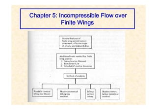
Central subject of wing theory:
Relation between wing shape and lift distribution
1. Analysis: determine the lift distribution for given wing shape
2. Design: determine wing shape for desired lift distribution
Lifting line theory: the wing is replaced by a vortex filament with
variable circulation (y) at the quarter-chord line + free vortices
12. OUTLINE FOR Chapter 5
Helmholtz Vortex
Theorem
• Consider the motion of an
inviscid fluid under the action
of conservative body force
(e.g. gravity, for which G=gz)
0
Dt
D
13. HELMHOTZ VORTEX THEOREM for Curved Vortex Filament
Reference: “Low Speed Aerodynamics From Wing Theory to
Panel method” by Katz aand Plotkin Chapter 2.9
Vortex line
Vortex tube
Vortex filament: a infinitesimal vortex
tube.
vorticity
velocity q
Variable defintion:
V - volume; q - velocity; - vorticity
0
Dt
D
14. 3-D Vortex Theory: the vortex filament
flow around a real wing uniform flow + vortices
V
2D: Straight vortex line: 3D general: curved vortex line
induced velocity
r
V
2
r P
15. 3-D Vortex Theory: Helmholtz’s vortex theorems
(compare the velocity induced by the vortex filament
to the magnetic field induced by an electrical current)
• The circulation strength remains constant along the filament
• a vortex filament cannot end in the flow, but:
– extends to infinity
– ends at a boundary
– forms a closed loop
consequence:
1
2
1
2
16. 3-D Vortex Theory: The Biot-Savart Law
The contribution dV of a filament section dl
to the induced velocity in P:
3
|
|
4 r
r
dl
V
d
θ
Direction: is perpendicular to and
Magnitude:
V
d dl r
dl
r
V
d 2
sin
4
|
|
Note: is the angle: r
dl
The Biot-Savart Law
17. Properties of a straight vortex filament segment (1)
A
B
B
A
dl
r
V 2
sin
4
P
h
r
l
A
B
θ
θ
-
2
sin
tan
sin
h
dl
h
l
h
r
)
cos
(cos
4
sin
4
B
B
A
A
h
d
h
V
Finite segment AB, constant
18. Properties of a straight vortex filament segment (2)
Note: A and B are the internal angles of ABP
)
cos
(cos
4
)
cos
(cos
4
B
A
B
A
h
h
V
P
h
B
B
θ
A
θ
B
B
Special cases:
• infinite vortex filament :
A = B = 0:
• semi-infinite filament:
A =90º; B = 0:
h
h
V
2
)
1
1
(
4
h
h
V
4
)
1
0
(
4
A
P
A
(same as 2D vortex)
A
A
19. 5.3 The Lifting-Line Theory
The Horseshoe vortex as a simple model of a finite wing
• the wing itself a bound vortex at the 1/4-chord line
is fixed, hence, experiences lift (L’ = V )
• the tip vortices free-trailing vortices
free to adjust to the local flow direction, no lift
• All vortices have the same circulation strength ;
• the free trailing vortices extend to infinity downstream
20. The single horseshoe vortex
• Downwash induced along the wing by
the two trailing (wing tip) vortices
)
2
/
(
4
)
2
/
(
4
)
(
y
b
y
b
y
w
Remarks:
• w < 0 when > 0: the induced flow is indeed downwards for positive lift
• Problems with the simple horseshoe-vortex model of a wing:
(y) = constant lift distribution
|w| at the tips not realistic!
2
2
)
2
/
(
4
)
(
y
b
b
y
w
right tip vortex left tip vortex
h
W
4
P
A
• Semi-infinite filament:
right tip vortex
left tip vortex
h
w
21. Extension of the horseshoe vortex model
towards the lifting-line model
• Instead of a single horseshoe vortex: superposition of many vortex systems
• Each vortex has a different span but the bound vortex segments coincide on the
same line and form the lifting line (= the wing)
• The circulation along the lifting line is no longer constant, but it varies along
the span in a stepwise fashion
• Extrapolate to infinite number of horseshoe vortices to obtain continuous (y)
22. Principle of the lifting line
• The wing is replaced by a bound vortex with (continuously) varying circulation (y)
• The trailing vortices create a ‘vortex wake’ in the form of a continuous vortex sheet
– local strength of the trailing vortex at position y is given by
the change in (y): d = (d/dy) dy
– the vortex sheet is assumed to remain flat (no deformation)
• Validity: good approximation for straight, slender wings at moderate lift
d
+ d
23. Determining the downwash of the lifting line (I)
Strength of the trailing vortex at position y
along the wing span:
• Take small segment of the lifting line, dy,
at position y
• Over this segment the change in circulation of
the lifting line is: d = (d/dy) dy
• This is equal to the strength of the trailing vortex
• The contribution dw to the induced velocity at position y0 :
Total velocity at position y0 induced by the entire vortex wake:
)
(
4 0 y
y
d
dw
dy
y
y
dy
d
y
w
b
b
2
/
2
/ 0
0
)
(
)
/
(
4
1
)
(
d = (d/dy) dy
(y)
dy
y0
y0 - y
w
y
24. Determining the induced angle of attack of the lifting line
induced angle of attack:
dy
y
y
dy
d
V
V
y
w
V
y
w
y
b
b
i
2
/
2
/ 0
0
0
1
0
)
(
)
/
(
4
1
)
(
)
)
(
(
tan
)
(
Total velocity at position y0 induced by
the entire vortex wake:
dy
y
y
dy
d
y
w
b
b
2
/
2
/ 0
0
)
(
)
/
(
4
1
)
(
25. The relation between circulation and wing shape
• Use ‘2D’ airfoil theory, but modified by the effective flow direction:
• From the relation between lift and circulation:
• combination:
]
[
]
[
)
( 0
0
0
eff
0
eff
L
i
L
l
l a
a
c
c
)
(
)
(
2
'
0
0
2
2
1
2
2
1 y
c
V
y
c
V
V
c
V
L
cl
i
L
l
a
c
0
0
dy
y
y
dy
d
V
y
y
c
V
a
y
y
b
b
L
2
/
2
/ 0
0
0
0
0
0
0
)
(
)
/
(
4
1
)
(
)
(
)
(
2
)
(
dy
y
y
dy
d
V
V
y
w
y
b
b
i
2
/
2
/ 0
0
0
)
(
)
/
(
4
1
)
(
)
(
The fundamental equation of Prandtl’s lifting-line theory
)
( 0
d
dc
a l
= const
26. Prandtl’s lifting-line equation (the wing equation)
Some remarks:
1. This equation describes the relation between circulation and wing properties
2. It is linear in
3. The circulation is proportional to V (Lift ~ V ~ V
2 )
4. For a wing without twist ( and L=0 are constant):
• circulation is proportional to – L=0
• for every value of the lift distribution has the same form
(which depends on a0(y), c(y) and b, therefore, on the wing shape)
• the total lift is zero when = L=0 and then: 0 along the spanwise yo
direction
5. For a wing with twist ( and L=0 are not constant): THIS IS NOT SO
• in particular: total zero lift is in general not accompanied by: 0 along
the spanwise yo direction
dy
y
y
dy
d
V
y
c
V
y
a
y
y
y
b
b
L
2
/
2
/ 0
0
0
0
0
0
0
0
)
(
)
/
(
4
1
)
(
)
(
)
(
2
)
(
)
(
27. Wing properties for given circulation (y)
1. Lift distribution:
2. Total lift:
3. Induced angle of attack:
4. Induced drag:
)
(
)
(
' y
V
y
L
2
/
2
/
2
/
2
/
)
(
'
b
b
b
b
dy
y
V
dy
L
L
2
/
2
/
)
(
2
b
b
L dy
y
S
V
S
q
L
C
dy
y
y
dy
d
V
y
b
b
i
2
/
2
/ 0
0
)
(
)
/
(
4
1
)
(
2
/
2
/
2
/
2
/
2
/
2
/
)
(
)
(
'
'
b
b
i
b
b
i
b
b
i
i dy
y
y
V
dy
L
dy
D
D
2
/
2
/
)
(
)
(
2
b
b
i
i
D dy
y
y
S
V
S
q
D
C i
28. The elliptical lift distribution (1)
2
0 )
2
/
(
1
)
(
b
y
y
Consider the following “elliptical” lift distribution:
(y) 0 = max.circulation
b/2
-b/2
y
d
b
dy sin
2
cos
2
b
y
)
0
(
)
(
coordinate
transformation:
sin
)
( 0
dy
y
y
dy
d
y
w
b
b
2
/
2
/ 0
0
/
4
1
)
(
Compute the downwash velocity from:
b
d
b
d
d
d
b
w
2
cos
cos
cos
2
cos
cos
/
2
1
)
( 0
0 0
0
0 0
0
=
Downwash and induced angle of attack
are constant over the span of the wing!
bV
V
w
i
2
0
29. The elliptical lift distribution (2)
sin
)
( 0
• Calculation of the total lift:
0 0
0
2
0
2
/
2
/
4
sin
2
sin
)
(
2
)
(
b
V
d
b
V
d
b
V
dy
y
V
L
b
b
d
b
dy sin
2
L
L
C
b
S
V
b
V
S
V
C
b
V
L
2
)
(
4
4
2
2
1
0
A
C
S
b
C
bV
L
L
i
)
/
(
2 2
0
A = b2/S: is called the ‘aspect ratio’ (AR) of the wing (“slankheid”)
typical values: 6-8 for subsonic aircraft
10-22 for glider aircraft
• The induced angle of attack
• Relation between
0 and CL:
30. The elliptical lift distribution (3)
Conclusions:
• The inducd drag is the “drag due to lift”
• Remember : total drag
• : quadratic dependence
• : large AR decreases induced drag
Calculation of the induced drag:
L
dy
L
dy
L
D i
b
b
i
b
b
i
i
2
/
2
/
2
/
2
/
'
'
Note that is constant here
A
C
C
C L
L
i
Di
2
A
CL
i
2
~ L
D C
C i
A
C i
D
1
~
i
D
d
D C
c
C
31. The elliptical lift distribution - wing shape
What wing shape can generate an elliptical lift distribution?
• assume: no twist: so and L-0 are constant
• assume: lift slope a0= dcl /d ( 2) is constant
• consequence: (with also i constant)
• required variation of the chord:
L
0
0 C
constant
]
[
L
i
l a
c
Remark: Proof:
2
/
2
/
2
/
2
/
1
1
b
b
l
b
b
l
l
L c
dy
c
S
c
dy
c
c
S
C
)
(
~
)
(
'
~
)
(
'
)
( y
y
L
c
q
y
L
y
c
l
)
(
)
(
' y
c
q
c
y
L l
L
C
l
c
The wing must have an elliptical planform
32. The elliptical wing shape
An elliptical wing planform: (note straight 1/4-chord line)
1/4-chord line
An elliptic lift distribution,
an elliptic wing planform
and a constant downwash
34. Aerodynamic properties of the elliptic wing
We found that: • (= constant)
• (= constant)
•
where:
L
C
l
c
A
CL
i
for an elliptic wing
for a general wing
]
[ 0
0
L
i
l a
c
d
dc
a l
0
Combining:
A
C
a
a
c
C L
L
L
i
l
L
0
0
0
0 ]
[
solve for CL:
note: CL = 0 when = L=0 and:
)
(
1 0
0
0
L
L a
A
a
C
A
a
a
d
dCL
/
1 0
0
35. Effect of Aspect Ratio on the lift-curve CL()
A
a
a
d
dC
a L
/
1 0
0
for an elliptic wing:
d
d
d
dc
d
dc
d
dC l
l
L eff
eff
.
The lift slope is reduced.
physical explanation: the downwash
reduces the effective angle of attack:
0
a
1
1
d
d i
36. The elliptical lift distribution - summary
• Constant downwash along the span
• Induced drag:
• Lift slope:
• effect of increasing the wing aspect ratio: - induced drag smaller
- lift-slope larger (a a0)
• Practical significance of the elliptical wing:
– optimum wing shape: minimal induced drag for given lift
– reference wing: reasonable approximation for real wings
A
CL
i
A
a
a
d
dC
a L
/
1 0
0
A
C
C
C L
L
i
Di
2
37. General lift distribution
cos
2
b
y
For the elliptical wing: with:
and:
sin
)
( 0
A
C
bV L
2
0
Describe the circulation of a general wing with a Fourier sine series:
n
A
bV
N
n
n sin
2
)
(
1
Note:
• The number of terms N should be taken “sufficiently large”
• = 0 at the tips
Questions to be answered:
• what are the aerodynamic properties (lift, induced drag)?
• what is the relation between the coefficients and the wing geometry?
a constant depending linearly
on CL, hence, on
constants that
depend on
Elliptical wing:
N=1; A1=CL/A
38. General lift distribution: total lift
n
A
bV
N
n
n sin
2
)
(
1
0
2
/
2
/
sin
)
(
)
(
2
d
S
V
b
dy
y
S
V
S
q
L
C
b
b
L
0
1
1
2
0 1
2
2
.
.
2
sin
sin
2
sin
sin
2
A
A
d
n
A
S
b
d
n
A
S
b N
n
n
N
n
n
Standard integrals:
= 0 when n 1
= /2 when n =1
A
A
CL
.
1
(Depends only on the first coefficient)
Calculation of the lift coefficient:
A
39. General lift distribution: downwash
n
A
bV
N
n
n sin
2
)
(
1
Standard integrals:
Calculation of the induced angle of attack: dy
y
y
dy
d
V
y
b
b
i
2
/
2
/ 0
0
)
(
)
/
(
4
1
)
(
d
n
nA
bV
bV
d
d
d
bV
N
n
n
i
0 0
1
0 0
0
cos
cos
cos
2
2
cos
cos
/
2
1
)
(
n
nA
bV
d
d N
n
n cos
2
1
0
0
sin
sin
n
0
0
1
0
sin
sin
)
(
n
nA
N
n
n
i
40. General lift distribution: induced drag
n
A
bV
N
n
n sin
2
)
(
1
0
2
/
2
/
sin
)
(
)
(
)
(
)
(
2
d
S
V
b
dy
y
y
S
V
S
q
D
C i
b
b
i
i
Di
0 1
1
2
sin
sin
sin
sin
2
d
n
nA
n
A
S
b N
n
n
N
n
n
= 0 when n m
= /2 when n = m
N
n
n
D nA
A
C i
1
2
Calculation of the induced-drag coefficient:
sin
sin
)
(
1
n
nA
N
n
n
i
0
1 1
2
sin
sin
2
d
m
n
A
A
n
S
b N
n
m
n
N
m
41. General lift distribution: summary and conclusions
A
A
CL
.
1
Conclusion:
• the elliptic wing ( = 0, e = 1) gives the lowest possible induced drag
(for given lift and aspect ratio)
N
n
n
N
n
n
D
A
A
n
A
A
nA
A
C i
2
2
1
2
1
1
2
1
0
where
)
1
(
2
2
1
2
N
n
n
L
D
A
A
n
A
C
C i
factor"
efficiency
span
"
the
1
)
1
(
1
where
:
or
2
e
Ae
C
C L
Di
42. The relation between the An and the wing geometry
Solve Prandtl’s wing equation:
• substitute:
Numerical solution method:
• Take a truncated series with N unknown coefficients: A1, A2,…AN
• Take N different spanwise locations on the wing where the equation is to
be satisfied: 1, 2, .. N; (but not at the tips, so: 0 < 1 < )
• System of N equations with N unknowns (Solve N N matix)
• Note: it is not possible to solve for only one coefficient, as in Chapter 4!
i
L
l
c
V
a
a
c
0
0
0
2
n
A
bV
N
n
n sin
2
)
(
1
sin
sin
)
(
1
n
nA
N
n
n
i
0
1
1
0 sin
sin
sin
4
L
N
n
n
N
n
n
n
nA
n
A
c
a
b
43. Numerical example of the wing equation (1)
• Consider: rectangular wing: c = constant; span = b; b/c = A;
without twist: = constant; L=0 = 0
• evaluate the wing equation at the N control points at i :
• The wing is symmetrical A2, A4,… are zero
i
N
n
n
i
n
A
n
a
A
sin
sin
4
1 0
N
i ...
,
2
,
1
)
sin(
sin i
i
)
(
sin
sin i
n
i
n n
A
n
A
number
even
is
n
for
0
sin
)
sin(
sin
:
even
is
n
n
i
n
i
n
i
n
A
n
A
n
n
A
n
A
If
number
odd
is
n
for
0
sin
)
sin(
)
sin(
sin
:
odd
is
n
n
i
n
i
n
i
n
i
n
A
n
A
n
A
n
n
A
n
A
If
0
/2
44. Numerical example of the wing equation (2)
• evaluate the wing equation at the N control points at i :
• The wing is symmetrical A2, A4,… are zero
– take only A1, A3,… as unknowns
– take only control points on half of the wing: 0 < i /2
• Example for N=3:
– take A1, A3, A5 as unknowns
– take control points (equidistant in ): 1 = /6, 2 = /3, 3 = /2
– take lift-slope of the airfoils a0 = 2, and wing aspect ratio A = 2
i
N
n
n
i
n
A
n
a
A
sin
sin
4
1 0
N
i ...
,
2
,
1
0 /2
/6 2/6
1
i 2
i 3
i
4/6 5/6
45. Numerical example of the wing equation (3)
– i=1, 1 = /6,
– i=2, 2 = /3,
– i=3, 3 = /2
i
N
n
n
i
n
A
n
a
A
sin
sin
4
1 0
N
i ...
,
2
,
1
)
6
/
5
sin(
)
6
/
sin(
5
4
)
6
/
3
sin(
)
6
/
sin(
3
4
)
6
/
sin(
)
6
/
sin(
1
4
5
0
3
0
1
0
A
a
A
A
a
A
A
a
A
)
3
/
5
sin(
)
3
/
sin(
5
4
)
3
/
3
sin(
)
3
/
sin(
3
4
)
3
/
sin(
)
3
/
sin(
1
4
5
0
3
0
1
0
A
a
A
A
a
A
A
a
A
)
2
/
5
sin(
)
2
/
sin(
5
4
)
2
/
3
sin(
)
2
/
sin(
3
4
)
2
/
sin(
)
2
/
sin(
1
4
5
0
3
0
1
0
A
a
A
A
a
A
A
a
A
46. Numerical example of the wing equation (3)
– i=1, 1 = /6,
– i=2, 2 = /3,
– i=3, 3 = /2
i
N
n
n
i
n
A
n
a
A
sin
sin
4
1 0
N
i ...
,
2
,
1
)
5
.
0
(
10
4
)
1
(
6
4
)
5
.
0
(
2
4 5
3
1 A
A
A
)
866
.
0
(
)
3
2
(
5
4
)
0
(
)
3
2
(
3
4
2
3
3
2
4 5
3
1 A
A
A
5
3
1 9
7
5 A
A
A
5
3
1 7
10
3 A
A
A
5
1 464
.
8
464
.
4 A
A
5
3
1 5
4
3
4
1
4 A
A
A
47. Numerical example: the rectangular wing (N=3)
• The set of equations becomes: with solution:
• Evaluation of the properties of the rectangular wing (with A = a0 = 2):
• Note: with 0.05: only 5% more induced drag than elliptical wing!
1
1
1
9
7
5
464
.
8
0
464
.
4
7
10
3
5
3
1
A
A
A
0040
.
0
0277
.
0
2316
.
0
5
3
1
A
A
A
572
.
4
1
A
A
CL
)
166
.
0
(
176
.
0
)
583
.
4
(
572
.
4
d
dC
a L
0
2
2
1
N
n
n
A
A
n
)
951
.
0
(
957
.
0
)
051
.
0
(
044
.
0
e
N=3 N=20
49. Effect of wing planform and aspect ratio
• Values of depend on planform and aspect ratio of the wing
)
1
(
2
A
C
C L
Di
)
1
)(
/
(
1 0
0
A
a
a
a
• Effect of wing planform on for
a tapered wing
A tapered wing with taper ratio
ct/cr = 0.3 is almost as good as
an elliptical wing!
example
50. Final conclusions
the effect of wing planform on the induced drag
• In order to reduce the induced drag it is more important
to increase the aspect ratio A than trying to approach the
elliptic lift distribution accurately
• A tapered wing with taper ratio ct/cr = 0.3 is almost as
good as an elliptical wing and is much easier to
manufacture
• Note that the parameter is a constant (i.e., independent
of ) only for a wing without twist!
• Remember:
total drag = induced drag + profile drag (~ viscosity)
)
1
(
2
A
C
C L
Di
51. Wing theory - a summary
• Lifting-line theory:
– The wing is replaced by a bound vortex at the 1/4-chord line of the wing with
varying circulation (y): the lifting line
– The trailing vortices form a flat sheet of distributed vorticity: the vortex wake
• Limitations of the classical theory:
– slender wings (large aspect ratio, or: span>>chord)
– straight wings (no wing sweep)
– moderate aerodynamic loading (no deformation of the vortex wake)
– linear relation
• Extensions:
(5.4) non-linear lifting-line theory:
(5.5) methods where the wing is represented by a vortex-sheet (instead of a line):
• lifting-surface / vortex-lattice methods
eff
~
l
c
)
( eff
l
c
52. 5.4 A numerical nonlinear lifting-line method
Given the wing shape and the angle of attack :
1. Divide the wing in spanwise positions: yn
2. Assume an initial circulation distribution
n=(yn), e.g. elliptical
3. Calculate the induced angle of attack:
4. Calculate:
5. Calculate lift coefficient:
6. Update circulation:
dy
y
y
dy
d
V
y
b
b n
n
i
2
/
2
/
)
(
)
/
(
4
1
)
(
)
(
)
(
eff n
i
n y
y
))
(
(
)
( eff n
l
n
l y
c
y
c
(evaluate the integral
numerically)
)
(
2
)
(
)
( n
l
n
n y
c
y
c
V
y
iterate until
convergence
(under relaxation
53. 5.5 Lifting-surface theory (principle)
Lifting line:
wing represented by a vortex filament
(only spanwise vorticity)
valid only for slender wings
wing
)
(y
Lifting surface:
wing represented by a vortex sheet with
distributed spanwise and chordwise
vorticity
V
wake
(streamwise
vorticity)
54. Lifting-surface theory - numerical implementation
• 3D vortex-panel methods:
– the wing is represented by panels with distributed vorticity
(three-dimensional extension of the vortex-panel method in section 4.9)
• Vortex-Lattice methods:
– distributed vorticity is concentrated into a lattice of horseshoe vortices
A single horseshoe vortex The vortex-lattice system on a finite wing