Kisan Call Centre - To harness potential of ICT in Agriculture by answer farm...
Tez
1. 1. INTRODUCTION
Heat Up processing is the basic step for the workload in melting and heat treatment for
further processing. It is also an energy-intensive process. Thus, correct predicition of the
temperature variation and distrubution in the workload is of significance to ensure the final
quality of the parts and to reduce energy consumption and time as well.
There has been a dramatic increase in recent years in theuse of comprehensive CFD
based computational tools to model industrial processes within the Chemical, Metallurgical,
andPower Generation Industries. For many in these industries, this has been a significant
change in philosophy. Historically, these industries relied on cold-flow experimental scale
models or 1-D zonal computational models to perform product/process R&D and to guide
scaling of pilot or laboratorydata for full size facilities. The motivations for the paradigm shift
are varied: pressures for increased productivity; global expansion of markets; tighter pollution
emission regulations; reducing the time to develop new products; and reducing the time to
bring new processes plants into full production.
It is established that mathematical model for the heating of workpiece in drying furnace
heat treatment furnace, while, the workpiece is assumed to be three dimensional and only
single workpiece is considered.
Using a reliable computational model which provides full coupling of all relevant
physical processes allows the engineer to determine sensitivities to design changes without
relying on simplified empirical models that are often extrapolated beyond the conditions for
which their validity has been proved. To properly model industrial systems requires
computational tools thatproperly describe the first-order physics and chemistry that drive the
system.
In recent years, the computational fluid dynamics (CFD) based on conservation
equations hasbecome a viable technique for process simulation So in this work we are going
to compute thetemperature profile generated Using CFD and GAMBIT for a given
temperature source, it canhelp to Compute the energy required and to optimize it.
1
2. 1.1.
Basics of Furnace
A furnace is an equipment used to melt metals for casting or to heat materials to change
their shape (e.g. rolling, forging) or properties (heat treatment).
Since flue gases from the fuel come in direct contact with the materials, the type of fuel
chosen is important. For example, some materials will not tolerate sulphur in the fuel. Solid
fuels generate particulate matter, which will interfere the materials placed inside the furnace.
For this reason:
Since flue gases from the fuel come in direct contact with the materials, the type of fuel
chosen is important. For example, some materials will not tolerate sulphur in the fuel. Solid
fuels generate particulate matter, which will interfere the materials placed inside the furnace.
For this reason:
Most furnaces use liquid fuel, gaseous fuel or electricity as energy input.
Induction and arc furnaces use electricity to melt steel and cast iron.
Melting furnaces for nonferrous materials use fuel oil.
Oil-fired furnaces mostly use furnace oil, especially for reheating and heat treatment of
materials.
Light diesel oil (LDO) is used in furnaces where sulphur is undesirable.
Furnace ideally should heat as much of material as possible to a uniform temperature
with the least possible fuel and labor. The key to efficient furnace operation lies in complete
combustion of fuel with minimum excess air. Furnaces operate with relatively low
efficiencies (as low as 7 percent) compared to other combustion equipment such as the boiler
(with efficiencies higher than 90 percent. This is caused by the high operating temperatures in
the furnace. For example, a furnace heating materials to 1200 oC will emit exhaust gases at
1200oC or more, which results in significant heat losses through the chimney.
For drying of solar cell metallization paste centrotherm photovoltaics provides drying
furnaces targeted for high volume production. Key features of centrotherm drying furnaces
include high throughput and uptime, powerful drying capabilities, modular build-up. Air
flows used for drying can be adjusted module-by-module precisely, which allows excellent
drying process setup and control.Our drying furnace comes with a powerful wafer cooling
stage. Cooling is achieved by closed loop air flows and air to cooling water heat exchangers.
This yields processed wafer delivery with nearly ambient temperature.Optionally, the
furnaces are available with exhaust condensers for exhaust gas cleaning.
2
3. An industrial furnace or direct fired heater is equipment used to provide heat for a
process or can serve as reactor which provides heats of reaction. Furnace designs vary as to its
function, heating duty, type of fuel and method of introducing combustion air. However, most
process furnaces have some common features.
Fuel flows into the burner and is burnt with air provided from an air blower. There can
be more than one burner in a particular furnace which can be arranged in cells which heat a
particular set of tubes. Burners can also be floor mounted, wall mounted or roof mounted
depending on design. The flames heat up the tubes, which in turn heat the fluid inside in the
first part of the furnace known as the radiant section or firebox. In this chamber where
combustion takes place, the heat is transferred mainly by radiation to tubes around the fire in
the chamber. The heating fluid passes through the tubes and is thus heated to the desired
temperature. The gases from the combustion are known as flue gas. After the flue gas leaves
the firebox, most furnace designs include a convection section where more heat is recovered
before venting to the atmosphere through the flue gas stack.
Radiation section:
Radiation section is where the tubes receive almost all its heat by radiation from the
flame. In avertical, cylindrical furnace, the tubes are vertical. Tubes can be vertical or
horizontal, placedalong the refractory wall, in the middle, etc., or arranged in cells.
Convection section:
The convection section is located above the radiant section where it is cooler to recover
additional heat. Heat transfer takes place by convection here, and the tubes are finned to
increase heat transfer. The first two tube rows in the bottom of the convection section and at
the top of the radiant section is an area of bare tubes (without fins) and are known as the
shield section, so named because they are still exposed to plenty of radiation from the firebox
and they also act to shield the convection section tubes, which are normally of less resistant
material from the high temperatures in the firebox.
Burner:
The burner in the vertical, cylindrical furnace as above is located in the floor and fires
upward. Some furnaces have side fired burners, e.g.: train locomotive. The burner tile is made
of hightemperature refractory and is where the flame is contained in. Air registers located
below theburner and at the outlet of the air blower are devices with movable flaps or vanes
that controlthe shape and pattern of the flame, whether it spreads out or even swirls around.
3
4. 1.2.
CFD Process
Preprocessing is the first step in building and analyzing a flow model. It includes
building the model (or importing from a CAD package), applying the mesh, and entering the
data. We used Gambit as the preprocessing tool in our project.
There are four general purpose products: FLUENT, Flowizard, FIDAF, and POLY
FLOW. FLUENT is used in most industries All Fluent software includes full post processing
capabilities.
1.3.
GAMBIT CFD Processor
Fast geometry modeling and high quality meshing are crucial to successful use
ofCFD.GAMBIT gives us both. Explore the advantage:
Ease of use
CAD/CAE Integration
Fast Modeling
CAD Cleanup
Intelligent Meshing
EASE-OF-USE
GAMBIT has a single interface for geometry creation and meshing that brings together all of
Fluent‟s preprocessing technologies in one environment. Advanced tools for journaling let
usedit and conveniently replay model building sessions for parametric studies.
4
5. 2. THEORY
2.1. Heat Transfer
Heat is defined as energy transferred by virtue of temperature difference or gradient.
Being a vector quantity, it flows with a negative temperature gradient. In the subject of heat
transfer, it is the rate of heat transfer that becomes the prime focus. The transfer process
indicates the tendency of a system to proceed towards equilibrium. There are 3 distinct modes
in which heat transfer takes place:
2.1.1. Heat Transfer by Conduction
Conduction is the transfer of heat between 2 bodies or 2 parts of the same body through
molecules. This type of heat transfer is governed by Fourier`s Law which states that – “Rate
of heat transfer is linearly proportional to the temperature gradient”. For 1-D heat conduction.
(1)
2.1.2. Heat Transfer by Radiation
Thermal radiation refers to the radiant energy emitted by the bodies by virtue oftheir
own temperature resulting from the thermal excitation of the molecules. It is assumed to
propagate in the form of electromagnetic waves and doesn‟t require any medium to travel.
The radiant heat exchange between 2 gray bodies at temperature T1 and T2 is given by:
(2)
2.1.3. Heat Transfer by Conduction
When heat transfer takes place between a solid surface and a fluid system in motion, the
process is known as Convection. When a temperature difference produces a density difference
that results in mass movement, the process is called Free or Natural Convection.
When the mass motion of the fluid is carried by an external device like pump, blower or
fan, the process is called Forced Convection. In convective heat transfer, Heat flux is given
by:
(3)
5
6. 2.1.3.1.
Reynolds Number
It is the ratio of inertial forces to the viscous forces. It is used to identify different flow
regimes such as Laminar or Turbulent.
(4)
2.1.3.2.
Nusselt Number
The nusselt number is a dimensionless number that measures the enhancement of heat
transfer from a surface that occurs in a real situation compared to the heat transferred if just
conduction occurred.
(5)
2.1.3.3.
Prandtl Number
It is the ratio of momentum diffusivity (viscosity) and thermal diffusivity.
(6)
2.1.3.4.
Grashof Number
It is the ratio of Buoyancy force to the viscous force acting on a fluid.
(7)
2.1.3.5.
Rayleigh Number
It is the product of Grashof number and Prandtl number. It is acdimensionless number
that is associated with buoyancy driven flow i.e. Free or Natural Convection. When the
Rayleigh number is below the critical value for that fluid, heat transfer is primarily inthe form
of conduction; when it exceeds the critical value, heattransfer is primarily in the form of
convection.
6
7. (8)
2.2. Computational Fluid Dynamics (CFD) and Fluent
Computational fluid dynamics (CFD) is one of the branches of fluid mechanics that uses
numerical methods and algorithms to solve and analyze problems that involve fluid flows.
The fundamental basis of any CFD problem is the Navier-Stokes equations, which define any
single-phase fluid flow. These equations can be simplified by removing terms describing
viscosity to yield the Euler equations. Further simplification, by removing terms describing
vorticity yields the full potential equations. Finally, these equations can be linearized to yield
the linearized potential equations.
2.2.1. Governing Equations
Continuity Equation:
(9)
Conservation of Momentum equation for an incompressible fluid is:
(10)
Energy Equation:
(11)
7
8. 2.2.2. Discretization Methods
The stability of the chosen discretization is generally established numerically rather than
analytically as with simple linear problems. Special care must also be taken to ensure that the
discretization handles discontinuous solutions gracefully. The Euler equations and NavierStokes equations both admit shocks, and contact surfaces. Some of the discretization methods
being used are:
2.2.2.1.
Finite Volume Method
This is the "classical" or standard approach used most often in commercial software and
research codes. The governing equations are solved on discrete control volumes. This integral
approach yields a method that is inherently conservative. (i.e., quantities such as density
remain physically meaningful)
A finite volume method (FVM) discretization is based upon an integral form of the PDE
to be solved (e.g. conservation of mass, momentum, or energy). The PDE is written in a form
which can be solved for a given finite volume (or cell). The computational domain is
discretized into finite volumes and then for every volume the governing equations are solved.
The resulting system of equations usually involves fluxes of the conserved variable, and thus
the calculation of fluxes is very important in FVM. The basic advantage of this method over
FDM is it does not require the use of structured grids, and theeffort to convert the given mesh
in to structured numerical grid internally is completely avoided. As with FDM, the resulting
approximate solution is a discrete, but the variables aretypically placed at cell centers rather
than at nodal points. This is not always true, as there arealso face-centered finite volume
methods. In any case, the values of field variables at nonstoragelocations (e.g. vertices) are
obtained using interpolation.
(12)
Where Q is the vector of conserved variables, F is the vector of fluxes (see Euler
equations or Navier-Stokes equations), V is the cell volume, and is the cell surface area.
8
9. 2.2.2.2.
Finite Element Method
This method is popular for structural analysis of solids, but is also applicable to fluids.
The FEM formulation requires, however, special care to ensure a conservative solution. The
FEM formulation has been adapted for use with the Navier-Stokes equations. In this method,
a weighted residual equation is formed:
(13)
A finite element method (FEM) discretization isbased upon a piecewise representation
of the solution in terms of specified basis functions. Thecomputational domain is divided up
into smaller domains (finite elements) and the solution ineach element is constructed from the
basis functions. The actual equations that are solved aretypically obtained by restating the
conservation equation in weak form: the field variables arewritten in terms of the basis
functions, the equation is multiplied by appropriate test functions,and then integrated over an
element. Since the FEM solution is in terms of specific basis functions, a great deal more is
known about the solution than for either FDM or FVM. This canbe a double-edged sword, as
the choice of basis functions is very important and boundaryconditions may be more difficult
to formulate. Again, a system of equations is obtained (usuallyfor nodal values) that must be
solved to obtain a solution.
Comparison of the three methods is difficult, primarily due to the many variations of all
three methods. FVM and FDM provide discrete solutions, while FEM provides a continuous
(upto a point) solution. FVM and FDM are generally considered easier to program than FEM,
butopinions vary on this point. FVM are generally expected to provide better conservation
properties, but opinions vary on this point also.
Where Ri is the equation residual at an element vertex i , Q is the conservation equation
expressed on an element basis, Wi is the weight factor and Ve is the volume of the element.
2.2.2.3.
Finite Difference Method
This method has historical importance and is simple to program. It is currently only used in
few specialized codes. Modern finite difference codes make use of an embedded boundary for
handling complex geometries making these codes highly efficient and accurate. Other ways to
handle geometries are using overlappinggrids, where the solution is interpolated across each
grid.
9
10. A finite difference method (FDM) discretization is based upon the differential form of
the PDE to be solved. Each derivative is replaced with an approximate difference formula
(that can generally be derived from a Taylor series expansion). The computational domain is
usually divided into hexahedral cells (the grid), and the solution will be obtained at each nodal
point. The FDM is easiest to understand when the physical grid is Cartesian, but through the
use of curvilinear transforms the method can be extended to domains that are not easily
represented by brick-shaped elements. The discretization results in a system of equation of the
variable at nodal points, and once a solution is found, then we have a discrete representation
of the solution.
(14)
Where Q is the vector of conserved variables, and F, G, and H are the fluxes in the x, y, and z
directions respectively.
2.2.3. Schemes to Calculate Face Value for variables
2.2.3.1.
Central Difference Scheme
This scheme assumes that the convective property at the interface is the average of the
values of its adjacent interfaces.
2.2.3.2.
The UPWIND Scheme
According to the upwind scheme, the value of the convective property at the interface is
equal to the value at the grid point on the upwind side of the face. It has got 3 sub-schemes i.e.
1st order upwind which is a 1st order accurate, 2nd order upwind which is 2ndorder accurate
scheme and QUICK (Quadratic Upwind Interpolation for convective kinematics) which is a
3rd order accurate scheme.
2.2.3.3.
The EXACT Solution
According to this scheme, in the limit of zero Peclet number, pure diffusion or
conduction problem is achieved and φ vs x variation is linear. For positive values of P, the
value of φ is influenced by the upstream value. For large positive values, the value of φ seems
tobe very close to the upstream value.
10
11. 2.2.3.4.
The EXPONENTIAL Scheme
When this scheme is used, it produces exact solution for any value of Peclet number and
for any value of grid points. It is not widely used because exponentials are expensive to
compute.
2.2.3.5.
The HYBRID Scheme
The significance of hybrid scheme can be understood from the fact that (i) it is
identical with the Central Difference scheme for the range -2 ≤ Pe ≤ 2 (ii) outside, it
reduces to the upwind scheme.
2.3.
How Does a CFD Code Work?
CFD codes are structured around the numerical algorithms that can be tackle fluid
problems. In order to provide easy access to their solving power all commercial CFD
packages include sophisticated user interfaces input problem parameters and to examine the
results. Hence all codes contain three main elements:
1. Pre-processing
2. Solver
3. Post-processing
2.3.1. Pre-processing
This is the first step in building and analyzing a flow model. Preprocessor consist of
inputof a flow problem by means of an operator –friendly interface and subsequent
transformationof this input into form of suitable for the use by the solver. The user activities
at the Preprocessing stage involve:
Definition of the geometry of the region: The computational domain.
Grid generation the subdivision of the domain into a number of smaller,
nonoverlapping sub domains (or control volumes or elements Selection of physical or
chemical phenomena that need to be modeled).
Definition of fluid properties
Specification of appropriate boundary conditions at cells, which
coincide with or touch the boundary. The solution of a flow problem (velocity,
pressure, temperature etc.) is defined at nodes inside each cell. The accuracy of CFD
solutions is governed by number of cells in the grid. In general, the larger numbers of
11
12. cells better the solution accuracy. Both the accuracy of the solution & its cost in terms
of necessary computer hardware & calculation time are dependent on the fineness of
the grid. Efforts are underway to develop CFD codes with a (self) adaptive meshing
capability. Ultimately such programs will automatically refine the grid in areas of
rapid variation.
GAMBIT (CFD PREPROCESSOR): GAMBIT is a state-of-the-art preprocessor for
engineering analysis. With advanced geometry and meshing tools in a powerful, flexible,
tightly-integrated, and easy-to use interface, GAMBIT can dramatically reduce preprocessing
times for manyapplications. Complex models can be built directly within GAMBIT‟s solid
geometry modeler, orimported from any major CAD/CAE system. Using a virtual geometry
overlay and advanced cleanup tools, imported geometries are quickly converted into suitable
flow domains. A comprehensive set of highly-automated and size function driven meshing
tools ensures that the best mesh can be generated, whether structured, multiblock,
unstructured, or hybrid.
2.3.2. Solver
The CFD solver does the flow calculations and produces the results. FLUENT,
FloWizard.
FIDAP, CFX and POLYFLOW are some of the types of solvers. FLUENT is used in
most industries. FloWizard is the first general-purpose rapid flow modeling tool for design
and process engineers built by Fluent. POLYFLOW (and FIDAP) are also used in a wide
range of fields, with emphasis on the materials processing industries. FLUENT and CFX two
solvers were developed independently by ANSYS and have a number of things in common,
but they also have some significant differences. Both are control-volume based for high
accuracy and rely heavily on a pressure-based solution technique for broad applicability. They
differ mainly in the way they integrate the fluid flow equations and in their equation solution
strategies. The CFX solver uses finite elements (cell vertex numerics), similar to those used in
mechanical analysis, to discretize the domain. In contrast, the FLUENT solver uses finite
volumes (cell centered numerics). CFX software focuses on one approach to solve the
governing equations of motion (coupled algebraic multigrid), while the FLUENT product
offers several solution approaches (density-, segregated- and coupled-pressure-based
methods)
The FLUENT CFD code has extensive interactivity, so we can make changes to the
analysisat any time during the process. This saves time and enables to refine designs more
12
13. efficiently.Graphical user interface (GUI) is intuitive, which helps to shorten the learning
curve and make the modeling process faster. In addition, FLUENT's adaptive and dynamic
mesh capability isunique and works with a wide range of physical models. This capability
makes it possible and simple to model complex moving objects in relation to flow. This solver
provides the broadestrange of rigorous physical models that have been validated against
industrial scale applications,so we can accurately simulate real-world conditions, including
multiphase flows, reacting flows,rotating equipment, moving and deforming objects,
turbulence, radiation, acoustics and dynamic meshing. The FLUENT solver has repeatedly
proven to be fast and reliable for a widerange of CFD applications. The speed to solution is
faster because suite of software enables usto stay within one interface from geometry building
through the solution process, to postprocessingand final output.
The numerical solution of Navier–Stokes equations in CFD codes usually implies a
discretization method: it means that derivatives in partial differential equations are
approximated by algebraic expressions which can be alternatively obtained by means of the
finite-difference or the finite-element method. Otherwise, in a way that is completely different
from the previous one, the discretization equations can be derived from the integral form of
the conservation equations: this approach, known as the finite volume method, is
implementedin FLUENT (FLUENT user‟s guide, vols. 1–5, Lebanon, 2001), because of its
adaptability to a widevariety of grid structures. The result is a set of algebraic equations
through which mass, momentum, and energy transport are predicted at discrete points in the
domain. In the freeboard model that is being described, the segregated solver has been chosen
so the governing equations are solved sequentially. Because the governing equations are nonlinearand coupled, several iterations of the solution loop must be performed before a
convergedsolution is obtained and each of the iteration is carried out as follows:
(1) Fluid properties are updated in relation to the current solution; if the calculation is at
the first iteration, the fluid properties are updated consistent with the initialized solution.
(2) The three momentum equations are solved consecutively using the current value for
pressure so as to update the velocity field.
(3) Since the velocities obtained in the previous step may not satisfy the continuity
equation, one more equation for the pressure correction is derived from the continuityequation
and the linearized momentum equations: once solved, it gives the correct pressure so
that continuity is satisfied. The pressure–velocity coupling is made by the SIMPLE algorithm,
as in FLUENT default options.
(4) Other equations for scalar quantities such as turbulence, chemical species and
13
14. radiation are solved using the previously updated value of the other variables; when
interphase coupling is to be considered, the source terms in the appropriate continuous
phaseequations have to be updated with a discrete phase trajectory calculation.
(5) Finally, the convergence of the equations set is checked and all the procedure is
repeated until convergence criteria are met.
The conservation equations are linearized according to the implicit scheme with respect
to the dependent variable: the result is a system of linear equations (with one equation foreach
cell in the domain) that can be solved simultaneously. Briefly, the segregated implicit method
calculates every single variable field considering all the cells at the same time. The
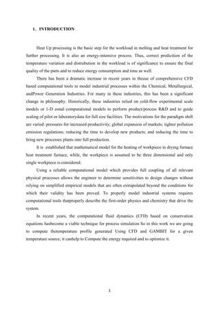
Figure 2.1:Algorithm of numerical approach used by simulation softwares
code stores discrete values of each scalar quantity at the cell centre; the face values must be
interpolated from the cell centre values. For all the scalar quantities, the interpolation is
carried out by the second order upwind scheme with the purpose of achieving high order
accuracy. The only exception is represented by pressure interpolation, for which the standard
method has been chosen.
14
15. 2.3.3. Post-processing
This is the final step in CFD analysis, and it involves the organization and interpretation
of the predicted flow data and the production of CFD images and animations. Fluent's
software includes full post processing capabilities. FLUENT exports CFD's data to third-party
postprocessors and visualization tools such as Ensight, Fieldview and TechPlot as well as to
VRML formats. In addition, FLUENT CFD solutions are easily coupled with structural codes
such as ABAQUS, MSC and ANSYS, as well as to other engineering process simulation
tools.
Thus FLUENT is general-purpose computational fluid dynamics (CFD) software
ideallysuited for incompressible and mildly compressible flows. Utilizing a pressure-based
segregated finite-volume method solver, FLUENT contains physical models for a wide range
of applications including turbulent flows, heat transfer, reacting flows, chemical mixing,
combustion, and multiphase flows. FLUENT provides physical models on unstructured
meshes, bringing you the benefits of easier problem setup and greater accuracy using
solution-adaptation of the mesh.
FLUENT is a computational fluid dynamics (CFD) software package to simulate fluid
flow problems. It uses the finite-volume method to solve the governing equations for a fluid.
Itprovides the capability to use different physical models such as incompressible or
compressible, inviscid or viscous, laminar or turbulent, etc. Geometry and grid generation is
done using GAMBIT which is the preprocessor bundled with FLUENT. Owing to increased
popularity ofengineering work stations, many of which has outstanding graphics capabilities,
the leading CFD are now equipped with versatile data visualization tools. These include:
Domain geometry & Grid display.
Vector plots.
Line & shaded contour plots.
2D & 3D surface plots.
Particle tracking.
View manipulation (translation, rotation, scaling etc.)
15
16. 2.3.4. Advantages of CFD
Major advancements in the area of gas-solid multiphase flow modeling offer substantial
process improvements that have the potential to significantly improve process plant
operations. Prediction of gas solid flow fields, in processes such as pneumatic transport lines,
risers, fluidized bed reactors, hoppers and precipitators are crucial to the operation of most
process plants. Up to now, the inability to accurately model these interactions has limited the
role that simulation could play in improving operations. In recent years, computational fluid
dynamics (CFD) software developers have focused on this area to develop new modeling
methods that can simulate gas-liquid-solid flows to a much higher level of reliability. As a
result, process industry engineers are beginning to utilize these methods to make major
improvements by evaluating alternatives that would be, if not impossible, too expensive or
time-consuming to trial on the plant floor. Over the past few decades, CFD has been used to
improve process design by allowing engineers to simulate the performance of alternative
configurations, eliminating guesswork that would normally be used to establish equipment
geometry and process conditions. The use of CFD enables engineers to obtain solutions for
problems with complex geometry and boundary conditions. A CFD analysis yields values for
pressure, fluid velocity, temperature, and species or phase concentration on a computational
grid throughout the solution domain. Advantages of CFD can be summarized as:
It provides the flexibility to change design parameters without the expense of
hardwarechanges. It therefore costs less than laboratory or field experiments, allowing
engineers to trymore alternative designs than would be feasible otherwise.
It has a faster turnaround time than experiments.
It guides the engineer to the root of problems, and is therefore well suited for
troubleshooting.
It provides comprehensive information about a flow field, especially in regions where
measurements are either difficult or impossible to obtain.
16
17. 3. SETUP
3.1.
Furnace
The furnace that is used in the project is a drying furnace. It is operated to heat material,
generally aluminum profiles, with intend to harden the strength of material ant its quality.
There are some identifications of the furnace:
FURNACE QUANTITY
Exterior Width
Exterior Height
Exterior Length
Isolatıon
Thermoblock Isolation
Types of Heat
Furnace Firebox
Thermal Capacity
Circulation Fan
Exhaust Fan
1,300 mm.
3,300 mm.
20,850 mm.
Fibreglass
150 mm Fibreglass
Natural Gasor LPGBurner
AISI 309-AISI 310
350,000 kcal / h
20,000 m3/h
1,500 m3/h
Table 3.1: Furnace Quantities
The furnace has a symetric profile, two inlets having a dimension of 700mmx400mm
and one outlet having a dimension of 2825mm x700mm. Hot air is blowed through the two
inlet with a high velocity to the furnace. On the other hand, it is vacuumed from the velocity
outlet. Profiles go through the furnace via conveyor, where profiles are hung on its hooks, wih
a constant amount of speed. The both side of the furnace has a single air curain to avoid the
heat loss. At bottom side of the furnace, there are 18 interoior cavities wihch are sized at
1000mmx150mm. Interior cavities oparetes circulation motion by directing particles of air.
These interiors are to serve air into to chamber of the furnace homogenously.
17
18. Figure3.1: Technical Drawing
3.2.
Geometry
To draw the furnace in Gambit, first of all, we started with creating faces at the bottom
side. The face created was copied by 20 times to get the bottom region ant cavities, then
complied the body part in Step 3. In Step 4 we dealed with curvelinear shape. Then, we
completed the parts below body part. After that, we substracted related faces from the whole
part.Finally, we created whole faces that we are going to use for boundry conditions. To
complete the above instructions, we followed the below commands:
Step 1
Geometry→Face→Create Face
Figuere 3.2: Face Command
Figure3.3: Face
18
22. Figure 3.12: The Final Drawing
3.3.
Zone
After finising geometry, we determine the boundry conditions to use them for next
operations.Also there are another type of boundry conditions called as continuum types. In
continuum condition, all volumes are selected as fluid. In the furnace, we have specified that;
Air Curtains
→
Hot Air Inlet
→
Air Curtains
→
Hot Air Outlet
→
Surrounding
→
Pressure Outlet 3
Walls and Interiors
22
24. Figure 3.15: Continuum Boundry
3.4.
Meshing
The last operation in GAMBIT is to be meshing. The object is meshed with 1.2 growth
rate, maximum size 2 and spacing 1. It also use Tet/Hybrid and TGrid.
For meshing, we gave size functions changing between a range. Size function are
applied because it is very hard and sometimes imposible to mesh because of details of
geometry. Size Function helps with resize more sensitively rather than normal size.
Size Function 1
It was chosen as from 30 to 250 with a1.2 growth rate. It is used on interiors as faces
and up and down volumes.
24
25. Size Function 2 – Size Function 3
Velocity inlet 1 and velocity inlet 2 are faces. Air curtains are said to be volumes and
size functions was from 30 to 250 with a growth rate of 1.2.
Size Function 4 – Size Function 5
Velocity inlet 3 and velocity inlet 4 were selected as faces and volumes are bottom large
volumes. It ranges from 40 to 100 with 1.2 growth rate.
Size Function 6
Pressure outlet 3 is selected as the face and volume is the upper CO (BURASI NE
ERAY?) It has a size function range of 50-250.
Figure 3.16: Mesh Volumes
25
27. Figure 3.19: Size Function Function 2-3
Figure 3.20: Size Function 4-5Figure 3.21: Size Function 6
27
28. 3.5.
Fluent
3.5.1. Case 1
In Case 1, we have used the boundry conditions symmetrically. The two inlets have the
same amount of mass of rate. Pressure outlet and velocity inlets boundries are to be as:
Pressure Outlet 1
Constant Gauge Pressure = - 19.97 Pa
Blackflow Turbulent Intensity= 10%
Blacflow Total Temperature= 430K
Hydraulic Diameter: 0.181
Pressure Outlet 3
Constant Gauge Pressure: - 5.81
Blackflow Turbulent Intensity: 10%
Blacflow Total Temperature: 430K
Hydraulic Diameter: 1.12
Velocity Inlet 1
Velocity Magnitude: 7 m/s
Turbulent Intensity: 10%
Hydraulic Diameter: 0.181
Velocity Inlet 3
Velocity Magnitude: 9.92 m/s
Turbulent Intensity: 10%
Hydraulic Diameter: 0.51
28
37. 3.5.2. CASE 2
In first case, we assumed that boundries are to be equal.On the other hand, the second
case we have changed mass flow rate of the two inlets as 9/10 proportion. To stabilize the
pressure, we have changed also the pressure outlet boundries.
Velocity Inlets
Figure 3.32.a: Velocity Inlet 3
Figure 3.32.b: Velocity Inlet3
37
41. 4. RESULTS
4.1.
Case1
Residuals are shown in Figure 3.21, x y and z velocities decreases linerarly and moves
constantly at 10-5 since 3000 iterations. Continuity and epsilon values become constant faster
at about 2000 iterations versus 10-4. Energy moves up and down in a frequency at first, then it
goes straight when iteration is about 1000 versus 10-5.
Figure 4.1: Residuals
Figure 4.2: Temperature Distribution
41
46. Figure 4.11: Wall Temperature Distribution (Outer)
Figure 4.12: Wall Temperature Distribution (Inner)
46
47. Mid-point Temperature
476 K
Inner Wall Temperature (min) – (max)
311 K -453 K
Outer Wall Temperature (min) – (max)
358 K – 458 K
Table 4.1: Results – Case 1
Inner Wall Temperature (min) – (max)
311 K – 451 K
Outer Wall Temperature (min) – (max)
341 K – 458 K
Table 4.2: Results – Case 2
47
48. 5. CONCLUSION
In this study, we have investigated the hot air motion of drying furnace and heat
transfer simulation.
There are two cases of furnace design to analyse. The first case represent a furance
control volume that has equal boundries acording to symetry axis. It can be said that it is the
uniform case. On the other hand, the second case of furnace analysis is seen that mass flowe
rayes of velocity inlets are changed with a proportion of 9 to 10. To balance the equilibrium
of pressure, air curtains on both sides has to have verse proportional of that.
We analysed the temperature at the center point of furnace. Because it would be the
average of the furnace especially for the first case. In addition, we have dealed with isolation
of the walls, chosen an inner and outer wall temperature.
In this result, we choose maximum values of inner and outer wall temperature as in
furnace firebox. It apperantly comes that the final results are aplicable and close to each case.
By contrast with Fluent, the inner and outer walls were chosen vice versa. Therefore,
results of inner temperature represent the outer wall temperature of the furnace.
For a new subject of thesis, it would be investigated that efficiency of heat transfer
could be investigated when aluminum profiles go through the hotspot. This report could be a
guide to the new project.
48
49. 6. REFERENCES
[1] Peeyush Agarwal. 2009 “Simulation of Heat Transfer Phenomenon in Furnace Using
FLUENT-GAMBIT” Page 23-25, National Institute of TechnologyRourkela
[2] Amritraj Bhanja, 2009 “Numerical Solution of Three Dimensional Conjugate Heat
Transfer in a Microchannel Heat Sink and CFD National Institute of Technology Rourkela
[3] Suhas V. Patankar, Numerical Heat Transfer and Fluid Flow
[4]www.fluent.com/ software/ gambit
[5]FLUENT documentation.
[6]Michael J. Bockelie, Bradley R. Adams, Marc A. Cremer, Kevin A. Davis,Eric G.
Eddings, James R. Valentine, Philip J. Smith, Michael P. Heap. „‟Computational
Simulations of Industrial Furnaces‟‟
[7]www.cfd-online.com
[8] Yunus A. Çengel, Michael A. Boles. „„ Thermodynamics An Engineering Aproach‟‟
5th Edition.
[9] Incropera. „„Fundamentals Heat and Mass Transfer‟‟ 6th Edition.
[10]hyperphysics.phy-astr.gsu.edu/hbase/tables/thrcn.html
[11]Zinedine Khatir, Joe Paton, Harvey Thompson, Nik Kapur, Vassili Toropov, Malcolm
Lawes, Daniel Kirk. 2011 „„Computational fluid dynamics (CFD) investigation of air flow
and temperature distribution in a small scale bread-baking oven‟‟ School of Mechanical
Engineering, University of Leeds, LS2 9JT, United Kingdom.
[11]confluence.cornell.edu/display/SIMULATION/FLUENT+Learning+Modules
[12]web.mst.edu/~isaac/aeme339.html/fs05_files/cyl_wake_tg.pdf
[13]Cornell University – Online Cources – Fluent
[14]Mark White, „„Fluid Mechanics‟‟ 5th Edition.
49