Download as PDF, PPTX

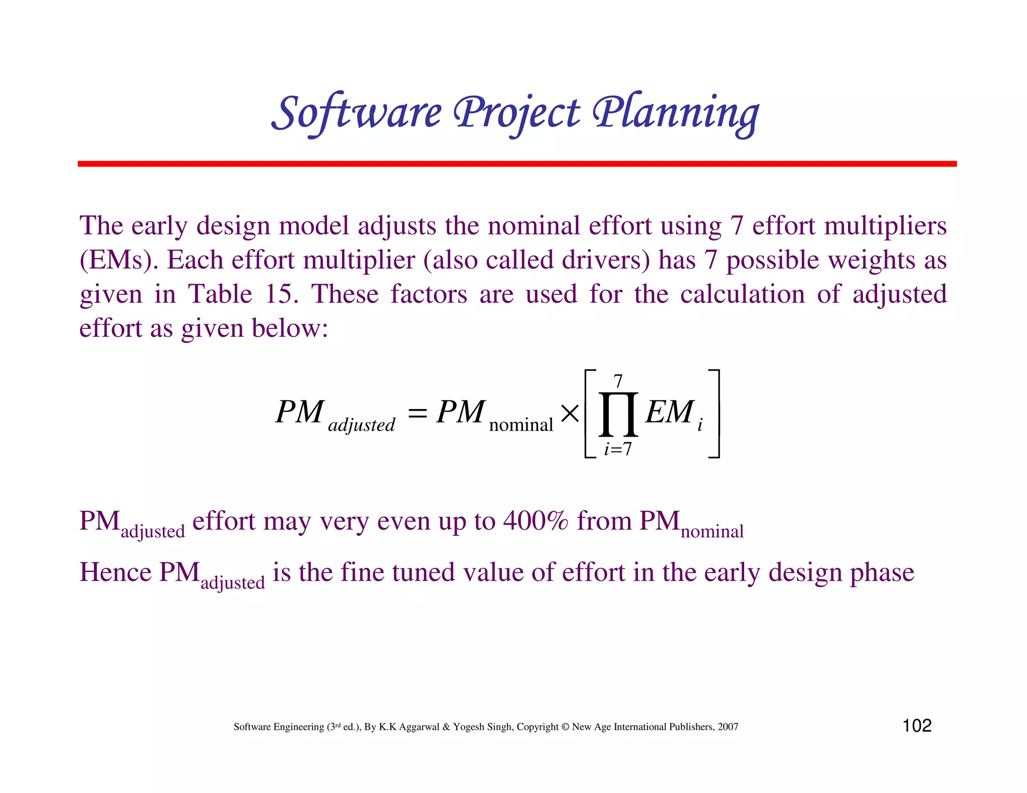
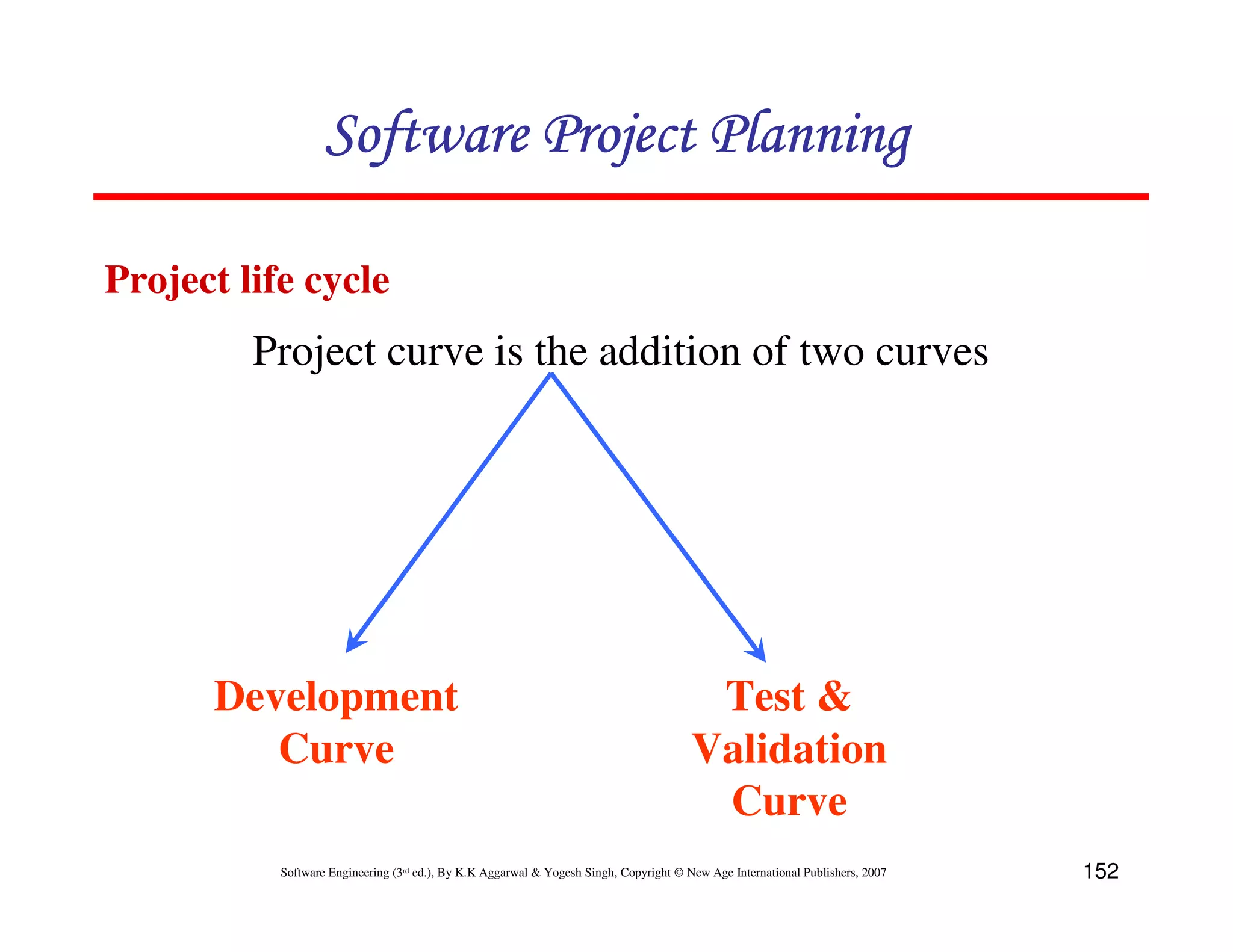
![Software Project Planning
Size Estimation Fig. 2: Function for sorting an array
1. int. sort (int x[ ], int n)
Lines of Code (LOC) 2. {
3. int i, j, save, im1;
If LOC is simply a count of 4. /*This function sorts array x in ascending order */
5. If (n<2) return 1;
the number of lines then 6. for (i=2; i<=n; i++)
figure shown below contains 7. {
8. im1=i-1;
18 LOC . 9. for (j=1; j<=im; j++)
10. if (x[i] < x[j])
11. {
When comments and blank
12. Save = x[i];
lines are ignored, the 13. x[i] = x[j];
program in figure 2 shown 14. x[j] = save;
15. }
below contains 17 LOC. 16. }
17. return 0;
18. }
Software Engineering (3rd ed.), By K.K Aggarwal & Yogesh Singh, Copyright © New Age International Publishers, 2007 5](https://image.slidesharecdn.com/chapter4softwareprojectplanning-120516010956-phpapp02/75/Chapter-4-software-project-planning-5-2048.jpg)
![Software Project Planning
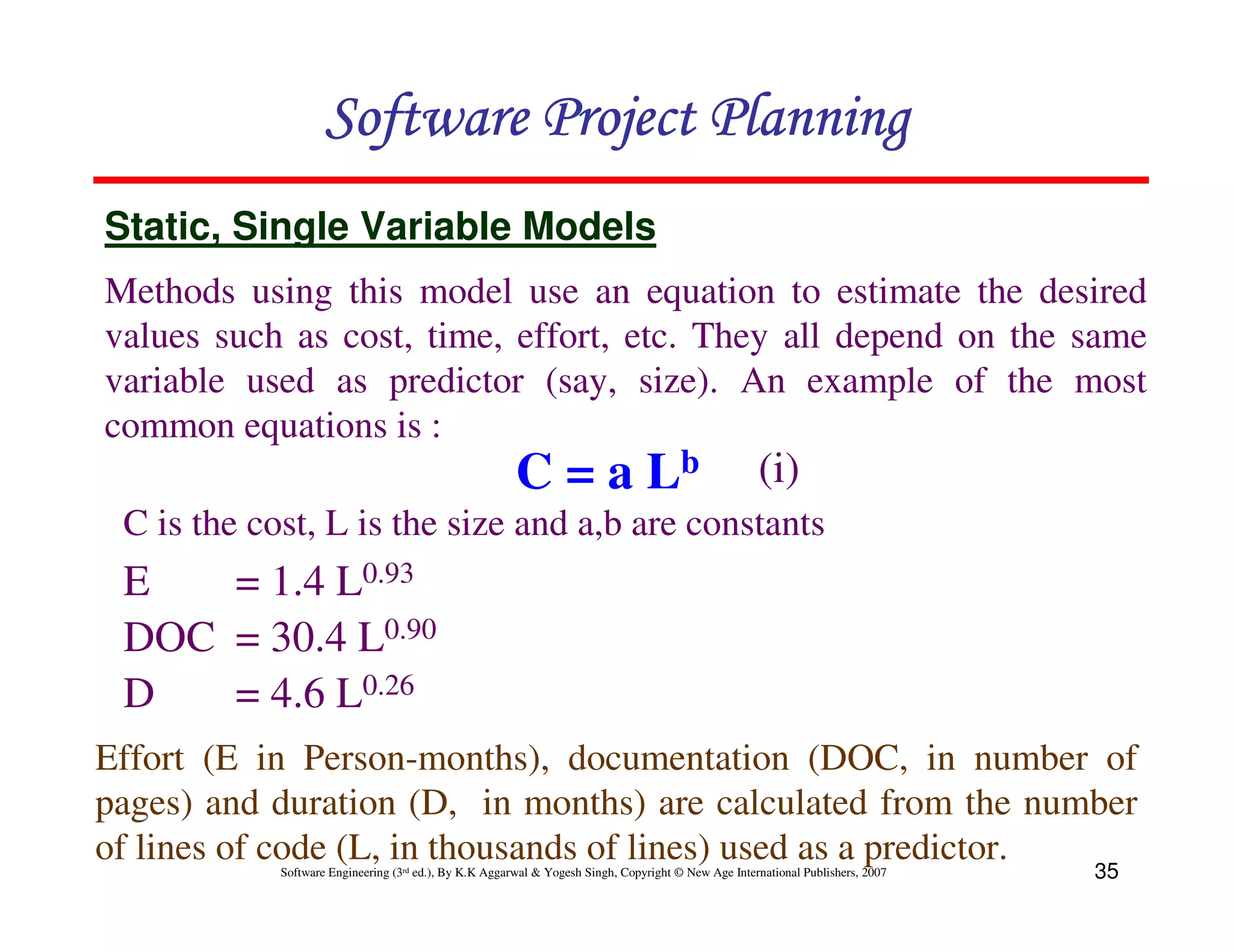
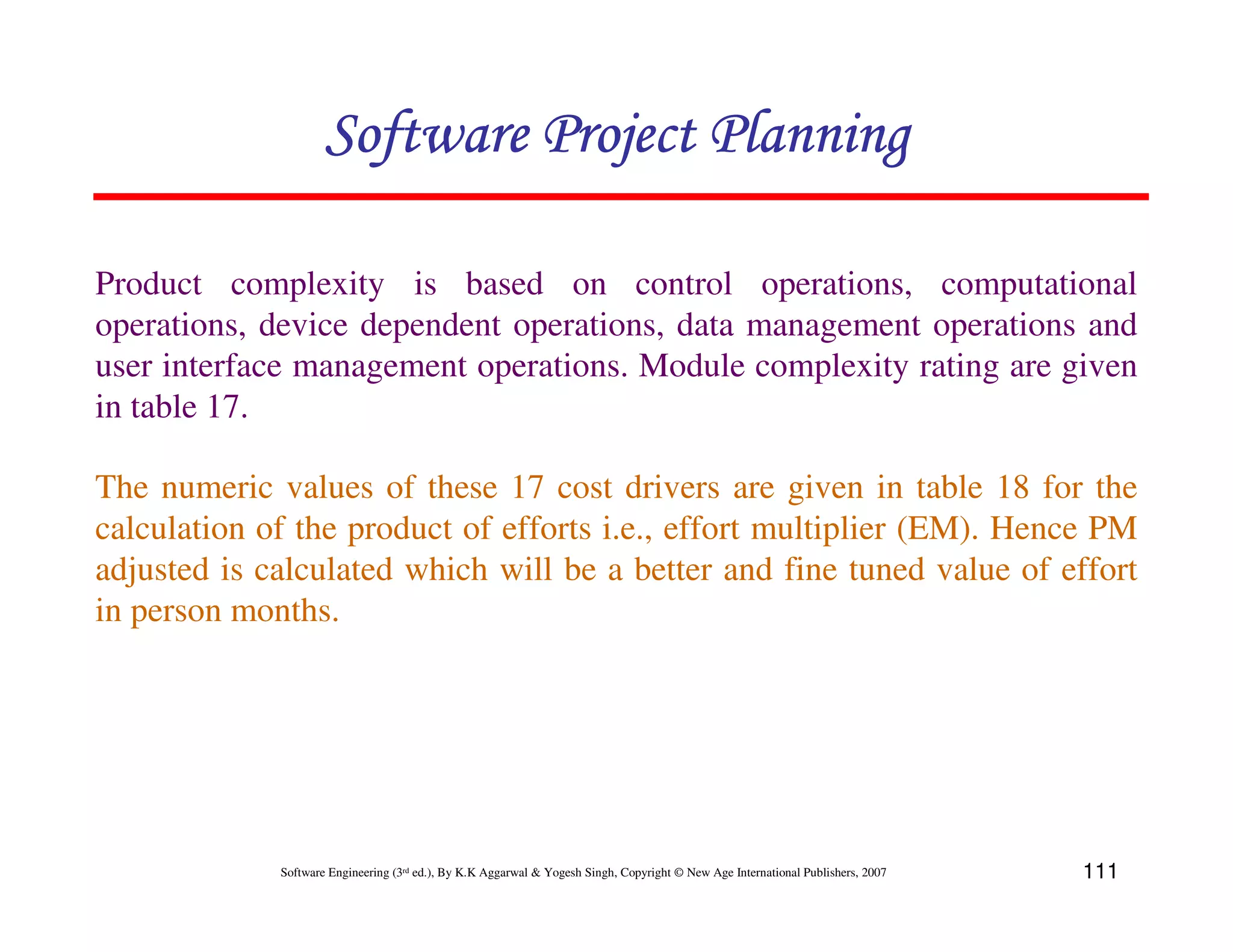
Organizations that use function point methods develop a criterion for
determining whether a particular entry is Low, Average or High.
Nonetheless, the determination of complexity is somewhat
subjective.
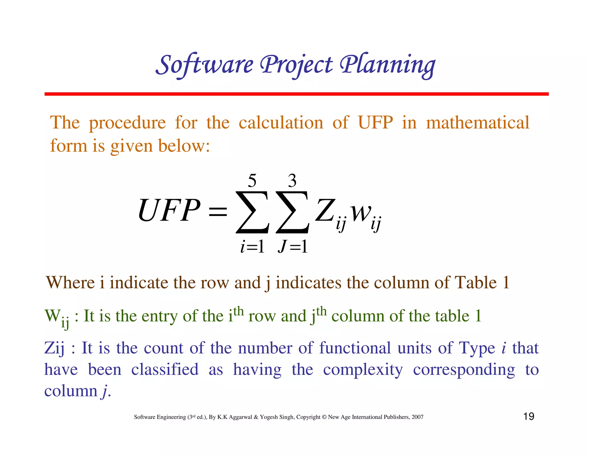
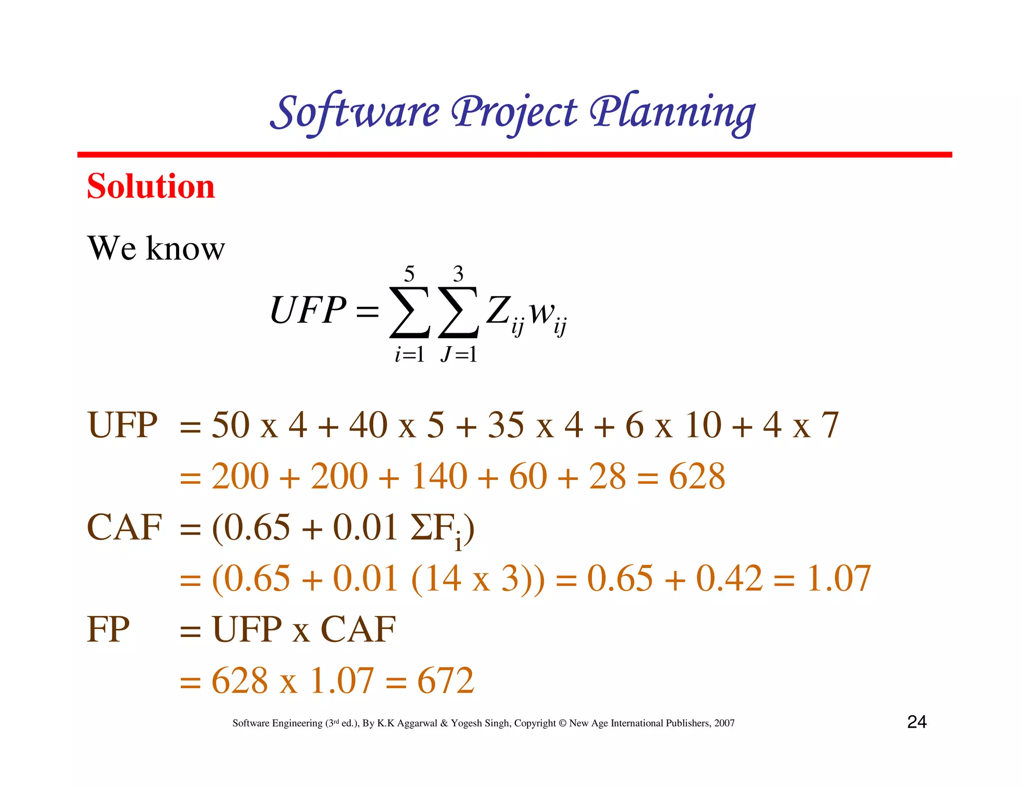
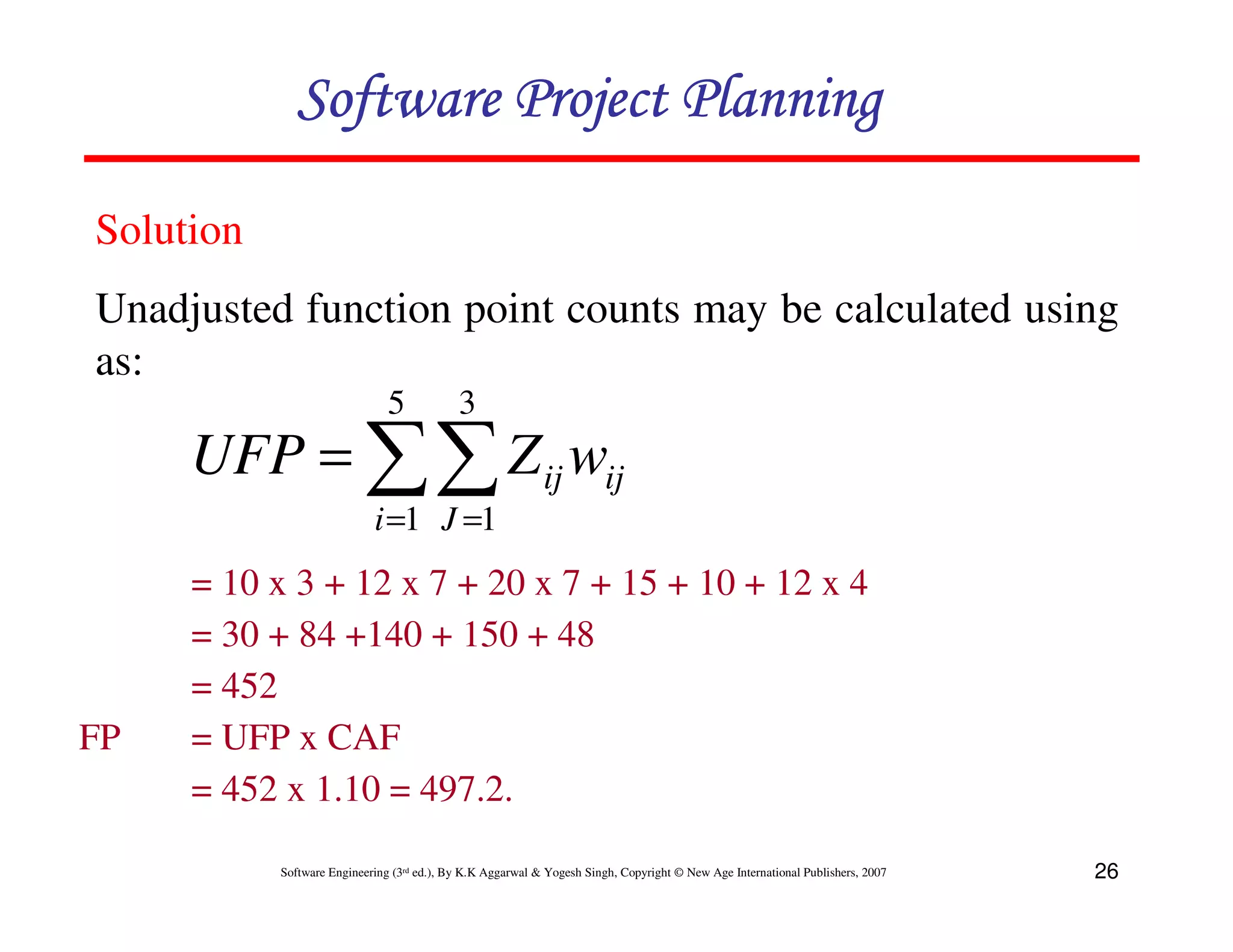
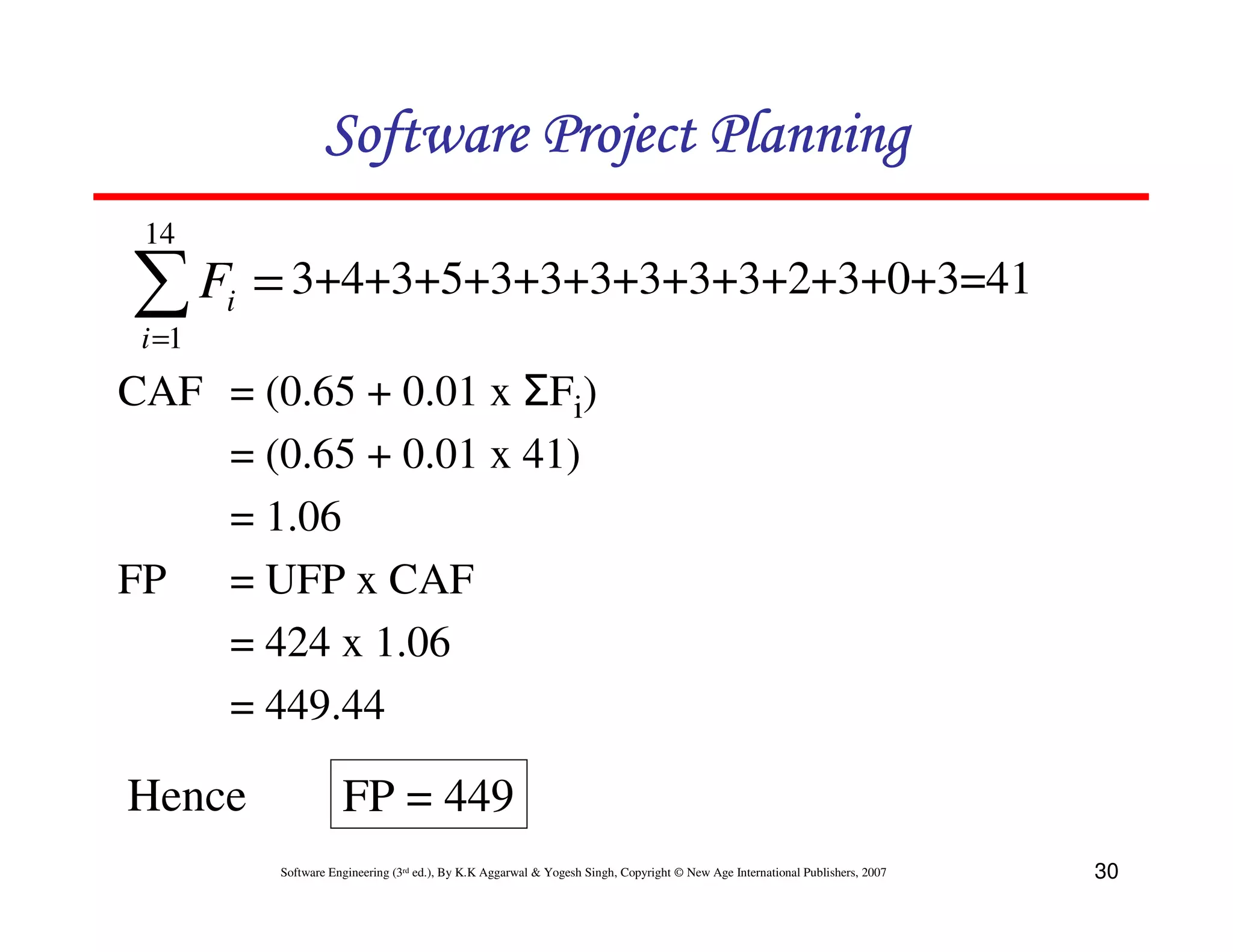
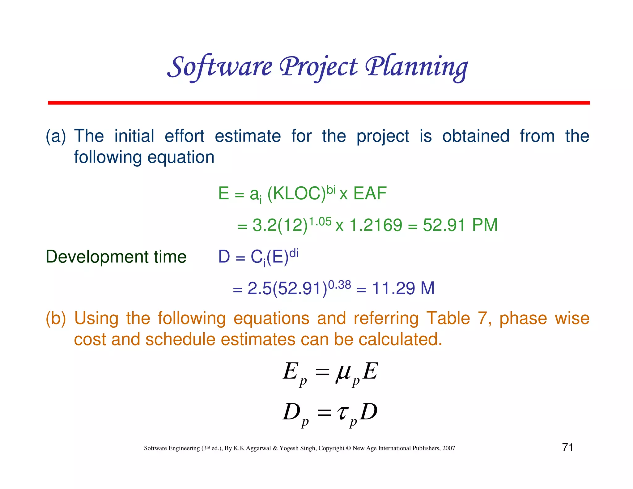
FP = UFP * CAF
Where CAF is complexity adjustment factor and is equal to [0.65 +
0.01 x ΣFi]. The Fi (i=1 to 14) are the degree of influence and are
based on responses to questions noted in table 3.
Software Engineering (3rd ed.), By K.K Aggarwal & Yogesh Singh, Copyright © New Age International Publishers, 2007 20](https://image.slidesharecdn.com/chapter4softwareprojectplanning-120516010956-phpapp02/75/Chapter-4-software-project-planning-20-2048.jpg)


![Software Project Planning
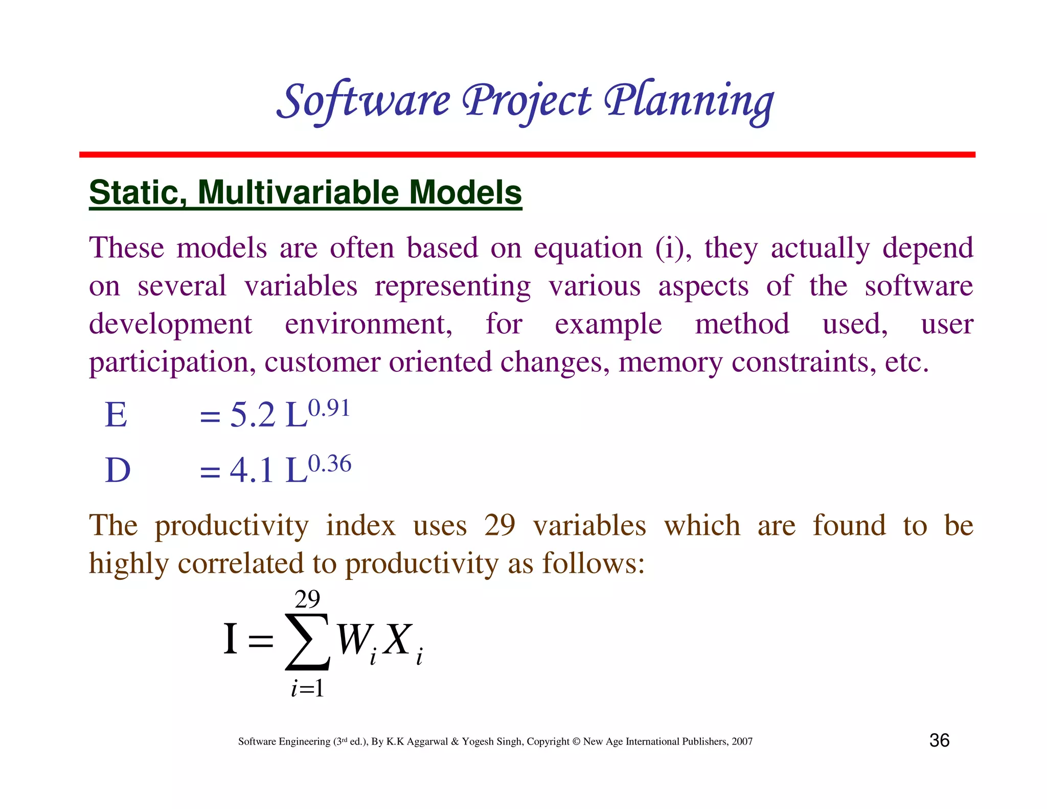
Schedule estimation
Development time can be calculated using PMadjusted as a key factor and the
desired equation is:
( 0.28+ 0.2 ( B − 0.091))] SCED %
TDEVnominal = [φ × ( PM adjusted ) ∗
100
where Φ = constant, provisionally set to 3.67
TDEVnominal = calendar time in months with a scheduled constraint
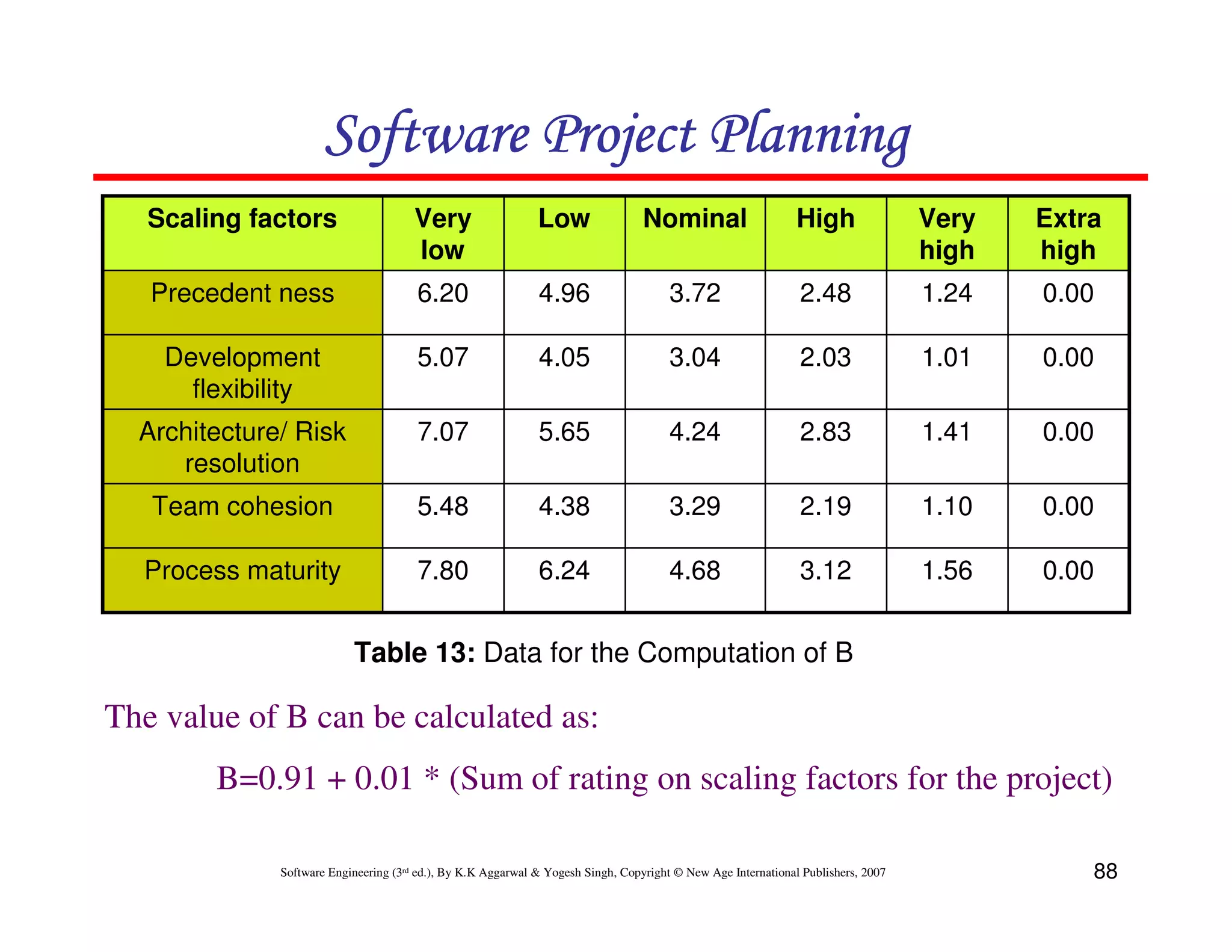
B = Scaling factor
PMadjusted = Estimated effort in Person months (after adjustment)
Software Engineering (3rd ed.), By K.K Aggarwal & Yogesh Singh, Copyright © New Age International Publishers, 2007 117](https://image.slidesharecdn.com/chapter4softwareprojectplanning-120516010956-phpapp02/75/Chapter-4-software-project-planning-117-2048.jpg)
![Software Project Planning
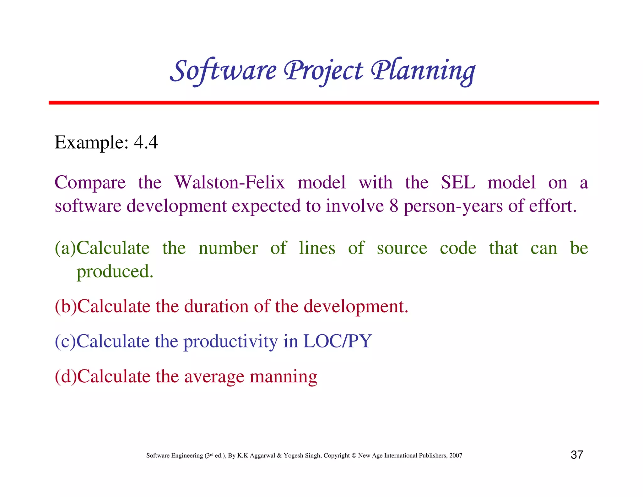
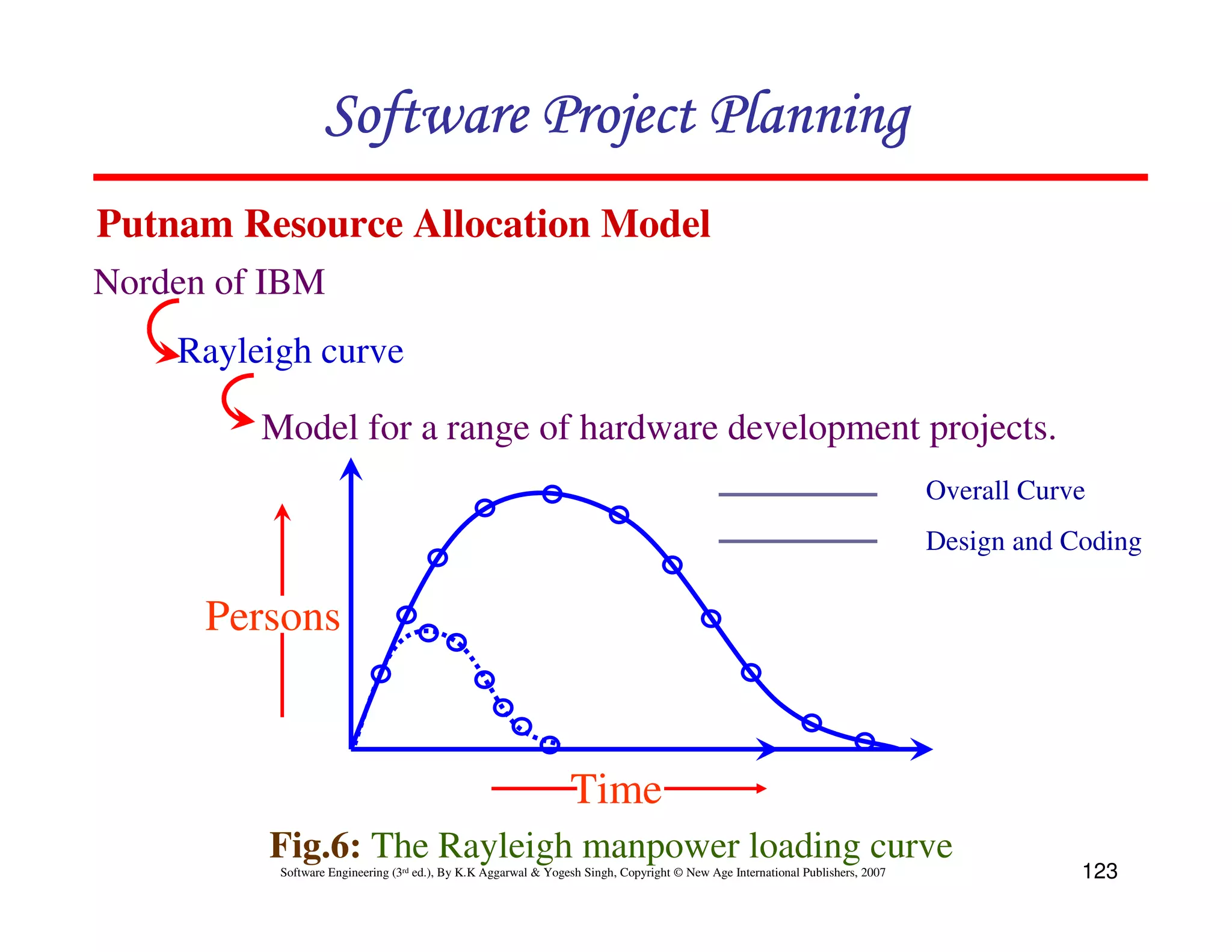
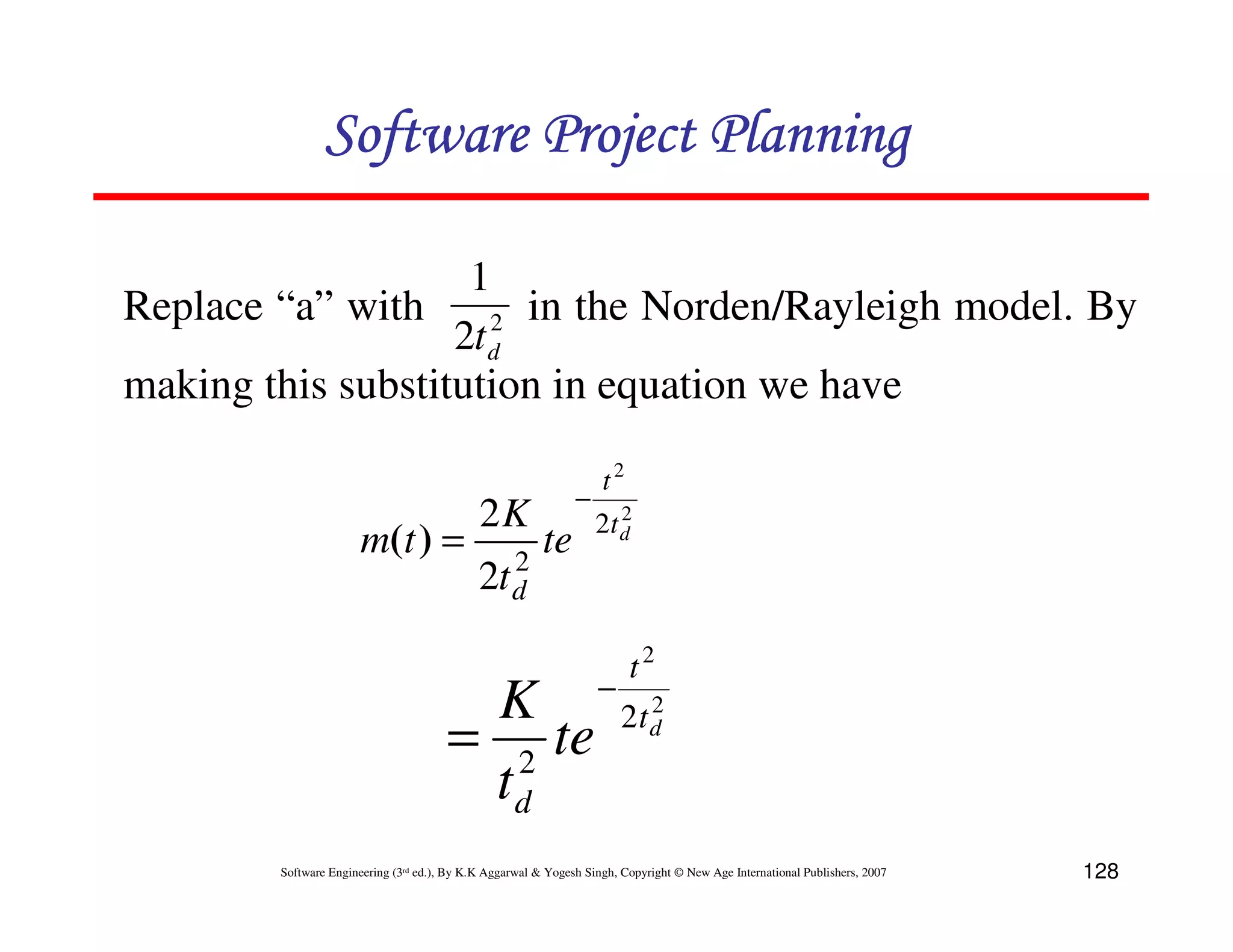
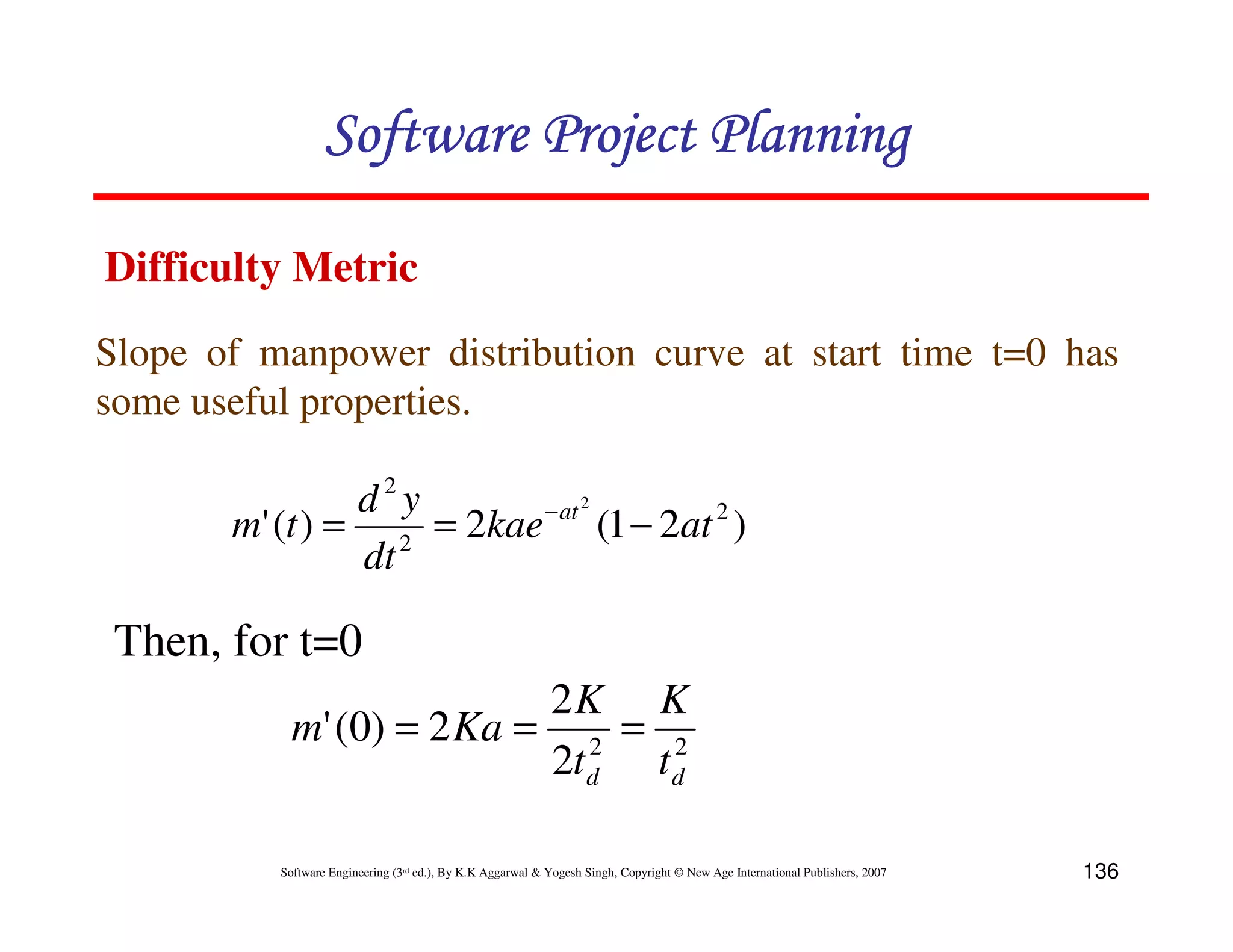
The Norden / Rayleigh Curve
The curve is modeled by differential equation
dy − at 2 --------- (1)
m(t ) = = 2kate
dt
dy
dt = manpower utilization rate per unit time
a = parameter that affects the shape of the curve
K = area under curve in the interval [0, ∞ ]
t = elapsed time
Software Engineering (3rd ed.), By K.K Aggarwal & Yogesh Singh, Copyright © New Age International Publishers, 2007 125](https://image.slidesharecdn.com/chapter4softwareprojectplanning-120516010956-phpapp02/75/Chapter-4-software-project-planning-125-2048.jpg)
![Software Project Planning
On Integration on interval [o, t]
y(t) = K [1-e-at2] -------------(2)
Where y(t): cumulative manpower used upto time t.
y(0) = 0
y(∞) = k
The cumulative manpower is null at the start of the project, and
grows monotonically towards the total effort K (area under the
curve).
Software Engineering (3rd ed.), By K.K Aggarwal & Yogesh Singh, Copyright © New Age International Publishers, 2007 126](https://image.slidesharecdn.com/chapter4softwareprojectplanning-120516010956-phpapp02/75/Chapter-4-software-project-planning-126-2048.jpg)
![Software Project Planning
d2y − at 2
= 2kae [1 − 2at 2 ] = 0
dt 2
2 1
td =
2a
“td”: time where maximum effort rate occurs
Replace “td” for t in equation (2)
2
td
E = y (t ) = k 1 − e 2 t d2 = K (1 − e − 0 .5 )
E = y ( t ) = 0 . 3935 k
1
a= 2
2t d
Software Engineering (3rd ed.), By K.K Aggarwal & Yogesh Singh, Copyright © New Age International Publishers, 2007 127](https://image.slidesharecdn.com/chapter4softwareprojectplanning-120516010956-phpapp02/75/Chapter-4-software-project-planning-127-2048.jpg)
![Software Project Planning
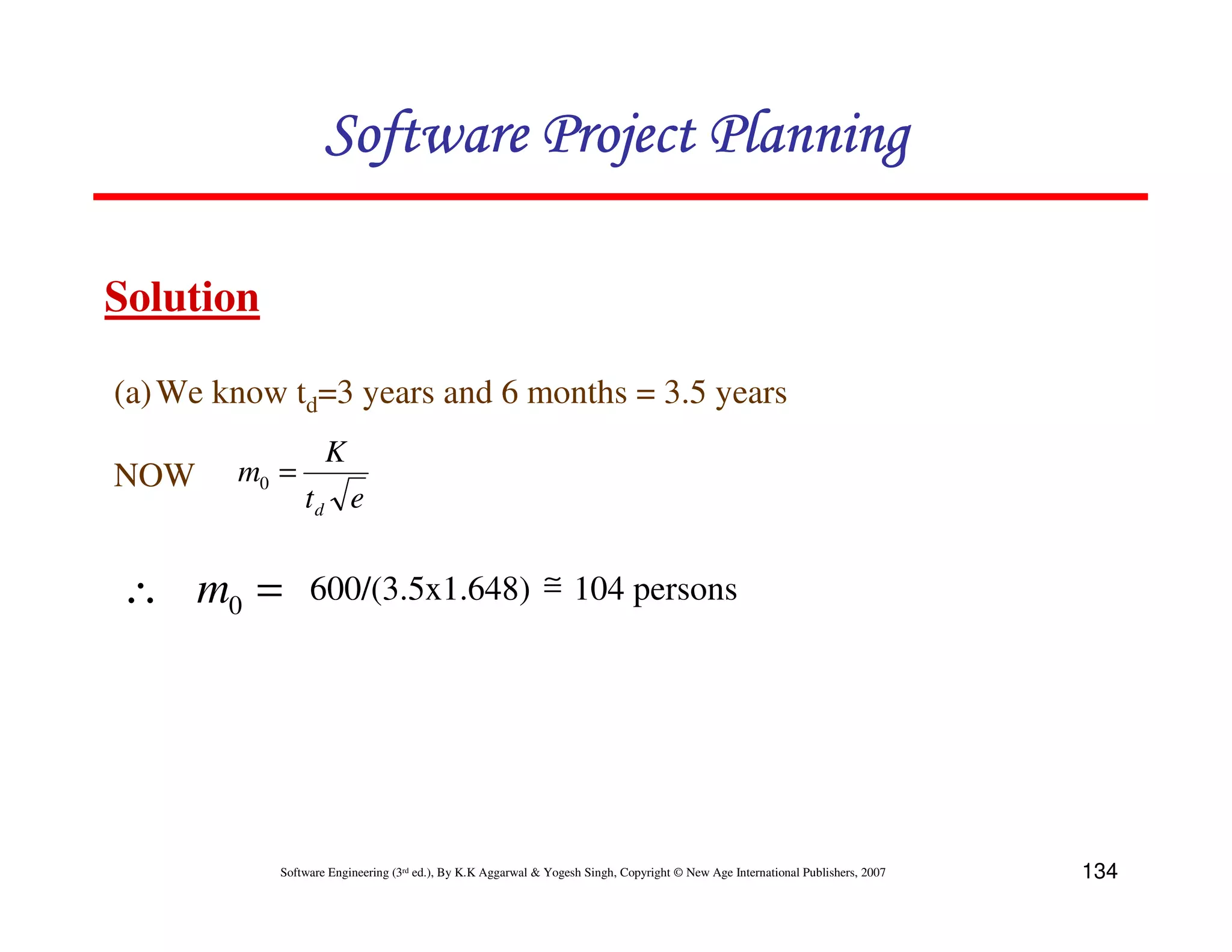
(b) We know
y (t ) = K 1 − e [ − at 2
]
t = 1 year and 2 months
= 1.17 years
1 1
a= 2
= 2
= 0.041
2t d 2 × (3.5)
y (1 .17 ) = 600 1 − e [ − 0 . 041 (1 . 17 ) 2
]
= 32.6 PY
Software Engineering (3rd ed.), By K.K Aggarwal & Yogesh Singh, Copyright © New Age International Publishers, 2007 135](https://image.slidesharecdn.com/chapter4softwareprojectplanning-120516010956-phpapp02/75/Chapter-4-software-project-planning-135-2048.jpg)
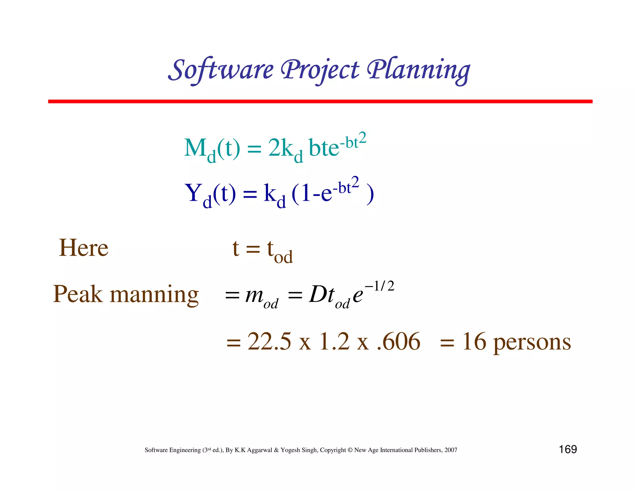
![Software Project Planning
∴ md (t) = 2kdbt e-bt2
yd (t) = Kd [1-e-bt2]
An examination of md(t) function shows a non-zero value of md
at time td.
This is because the manpower involved in design & coding is
still completing this activity after td in form of rework due to
the validation of the product.
Nevertheless, for the model, a level of completion has to be
assumed for development.
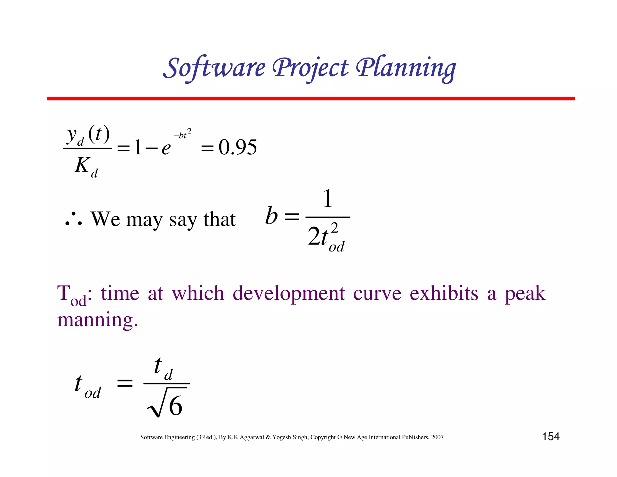
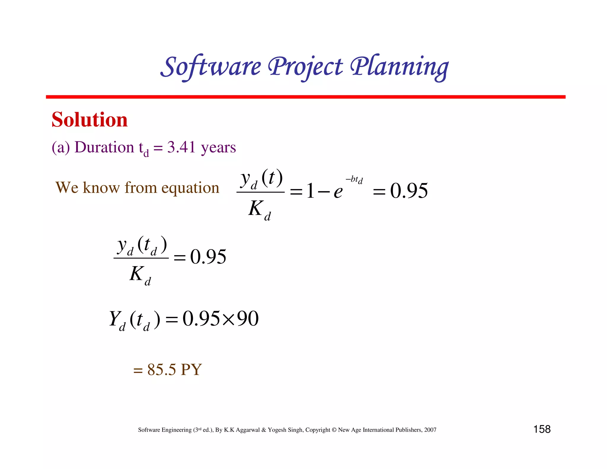
It is assumed that 95% of the development will be completed
by the time td.
Software Engineering (3rd ed.), By K.K Aggarwal & Yogesh Singh, Copyright © New Age International Publishers, 2007 153](https://image.slidesharecdn.com/chapter4softwareprojectplanning-120516010956-phpapp02/75/Chapter-4-software-project-planning-153-2048.jpg)
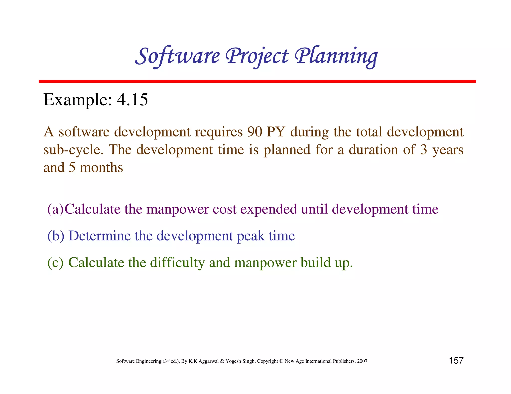


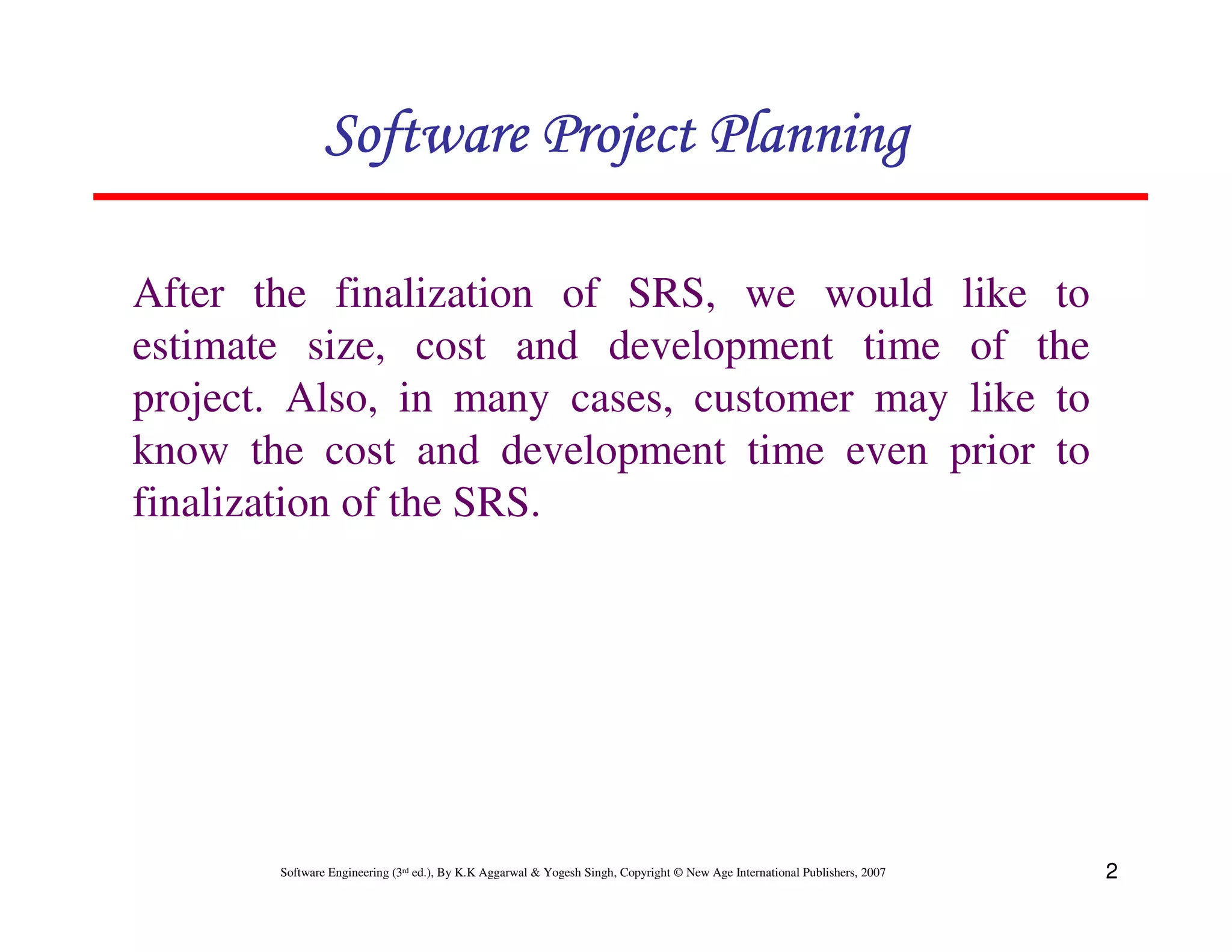
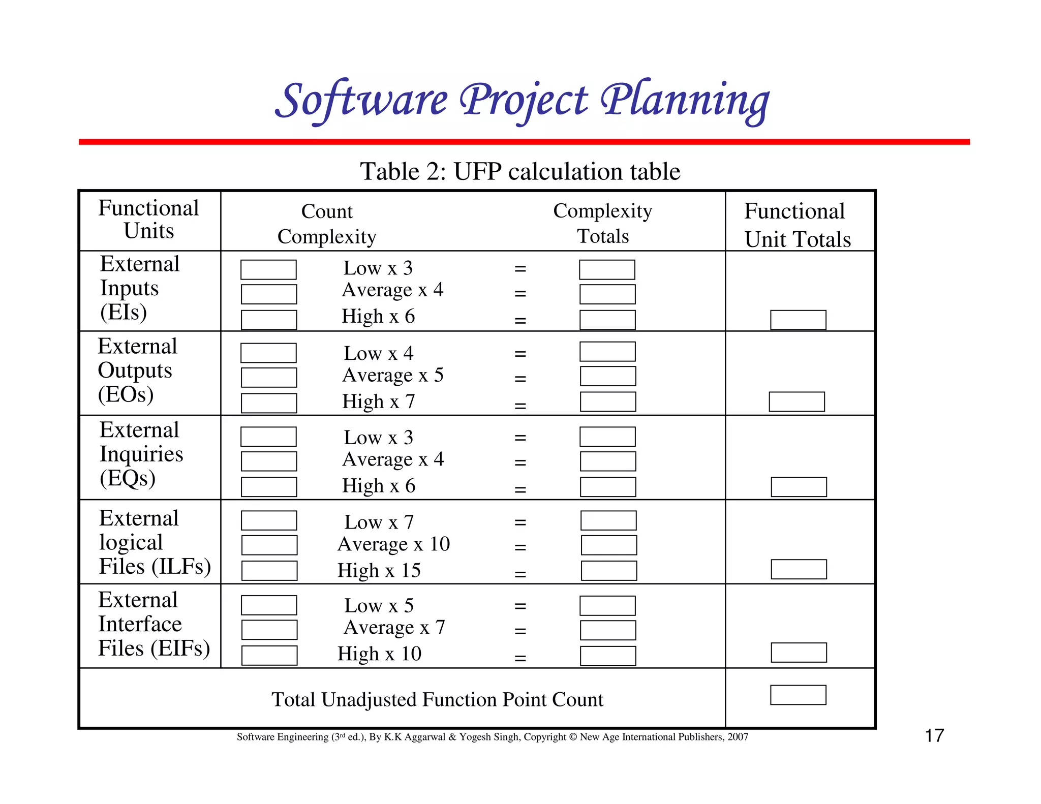
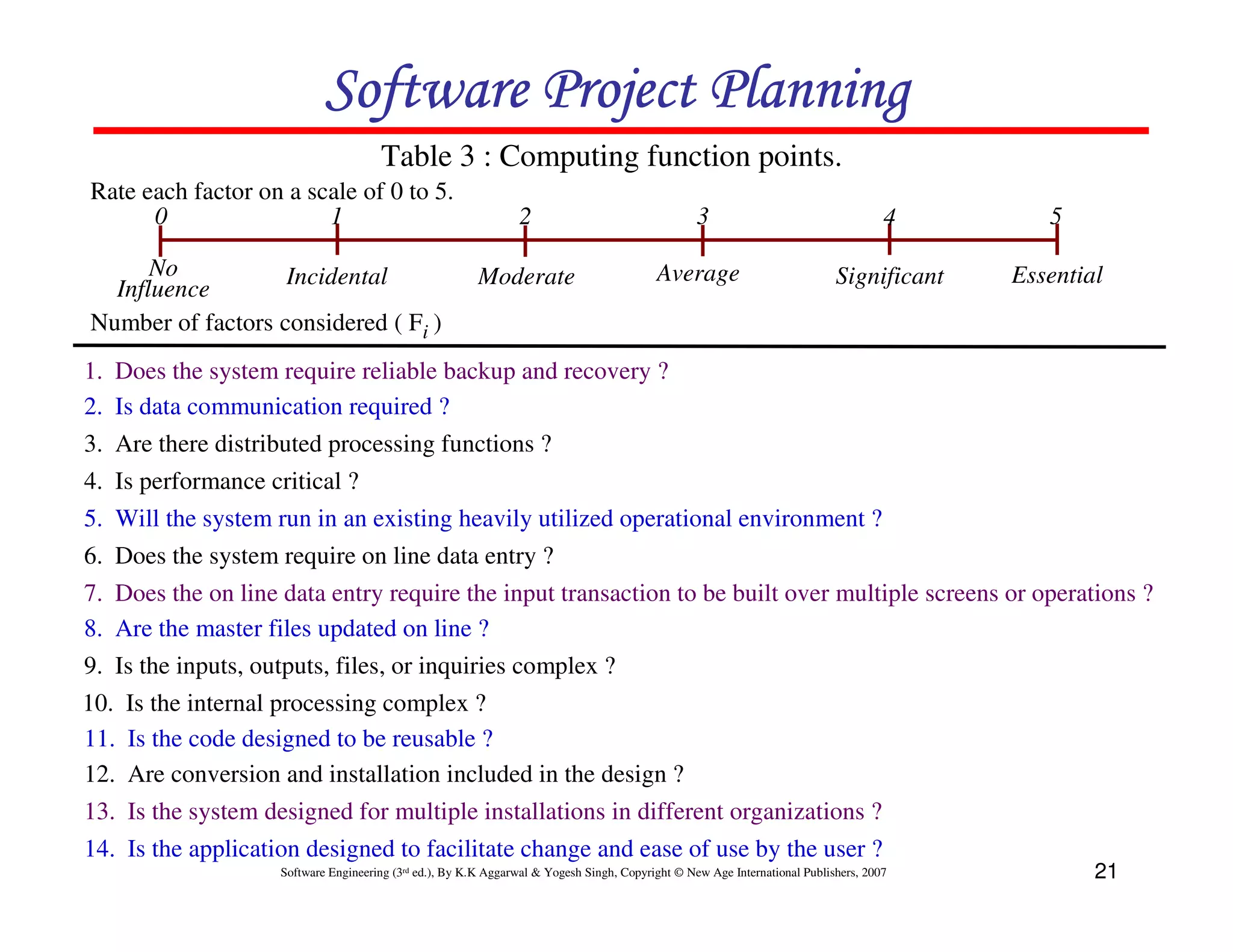
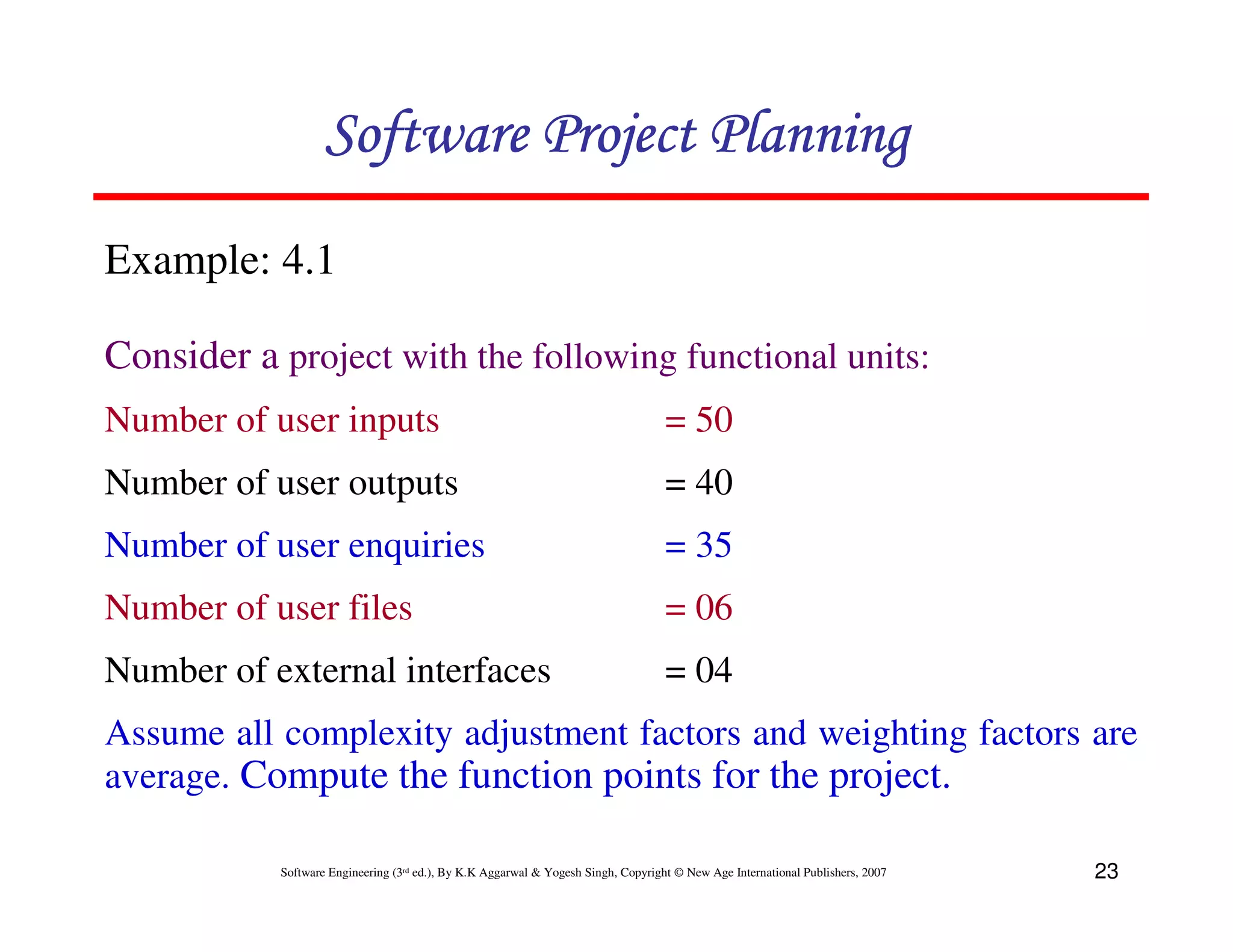
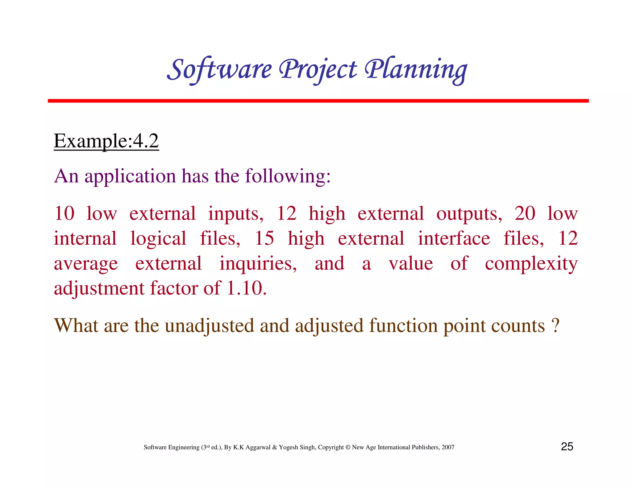
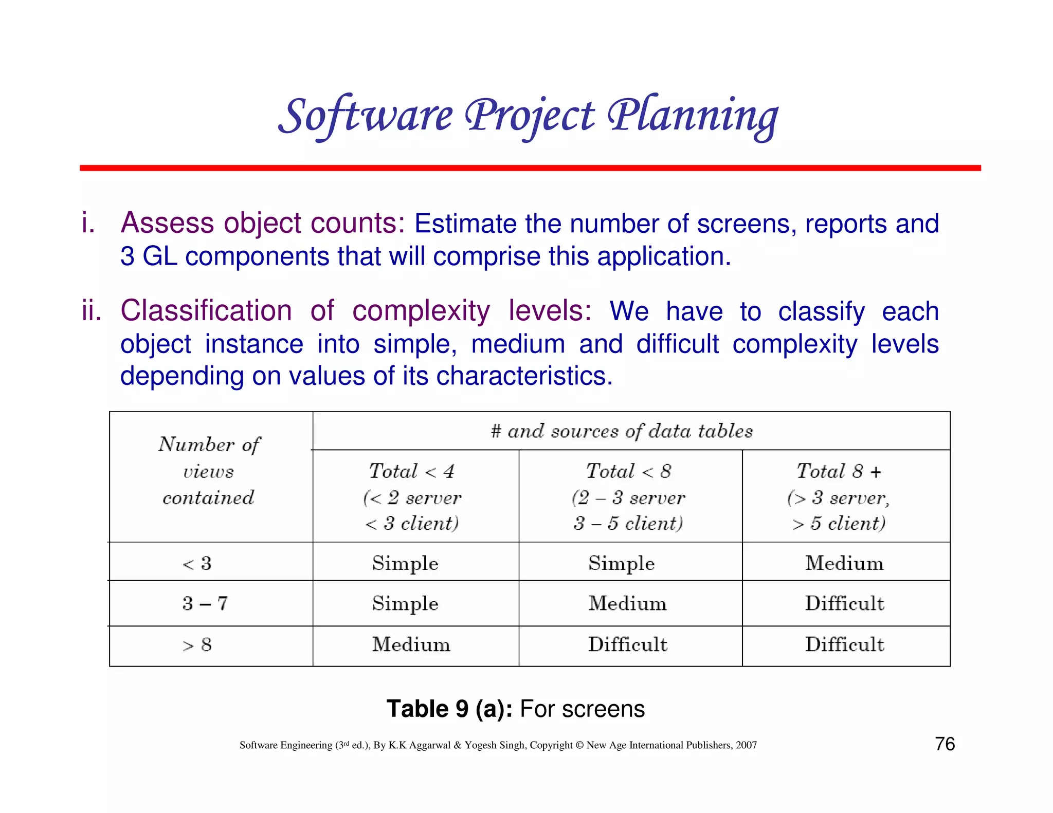
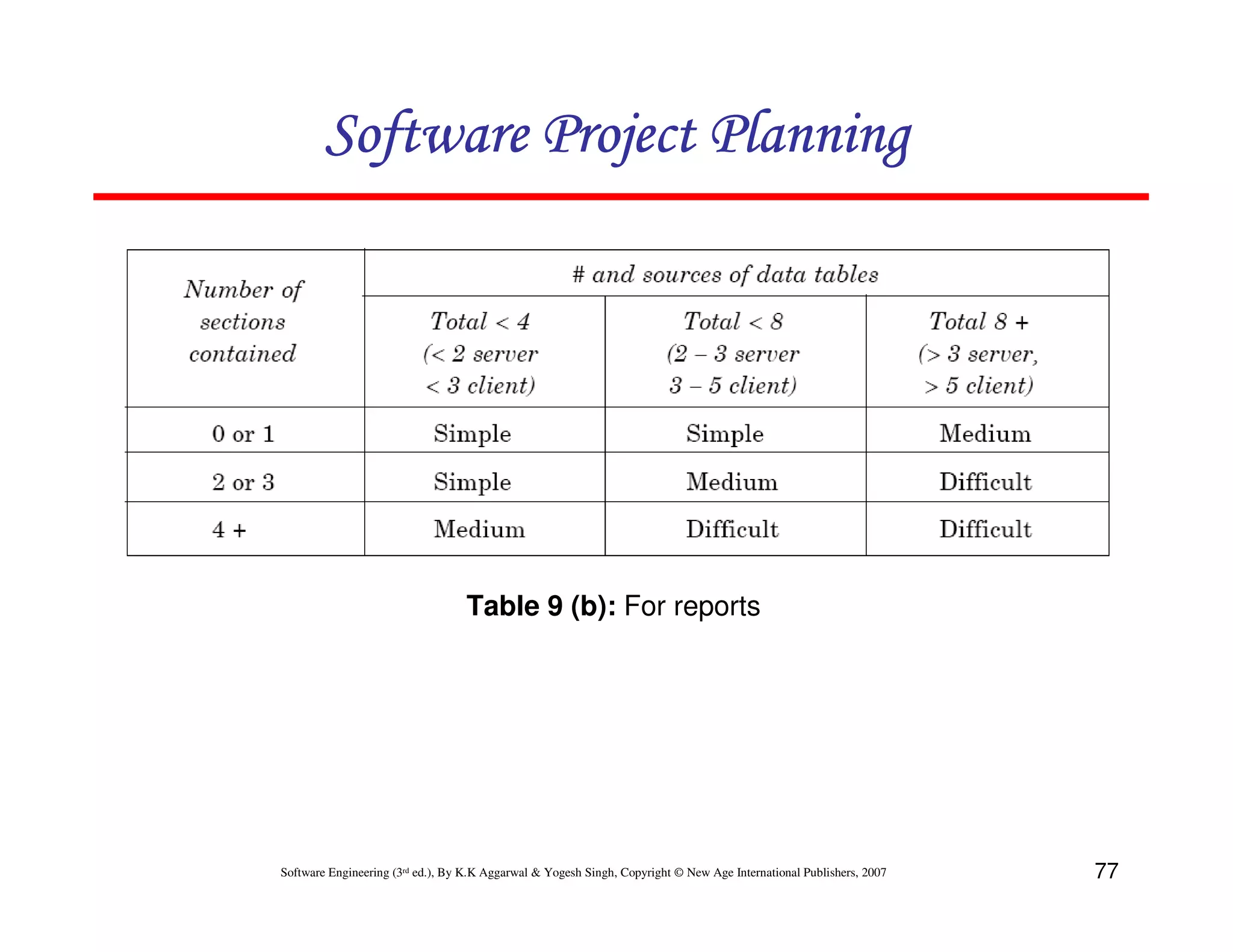
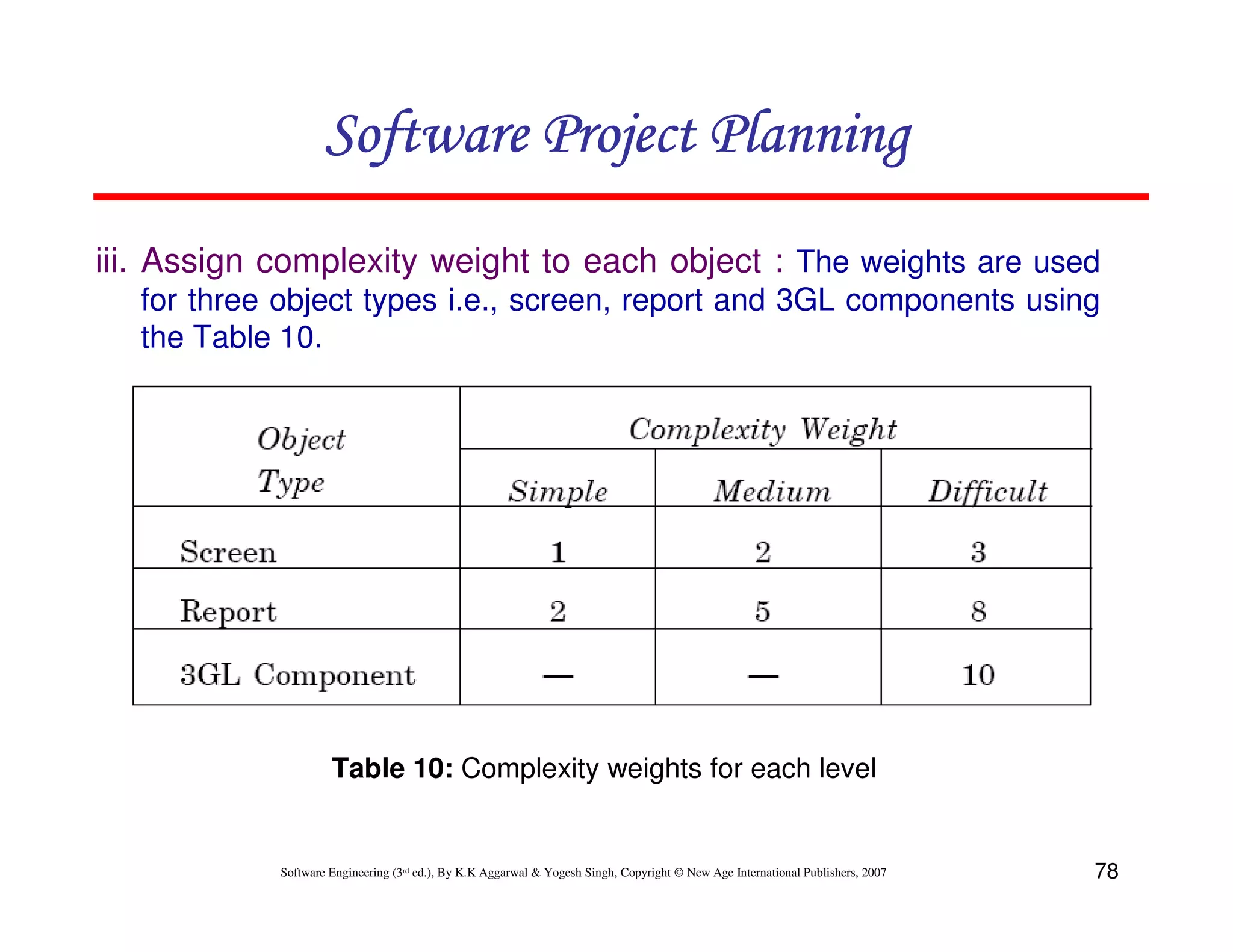
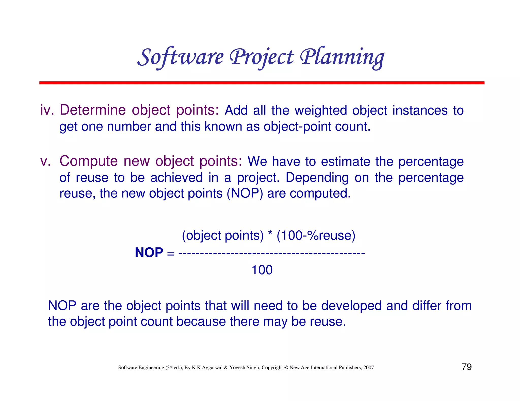
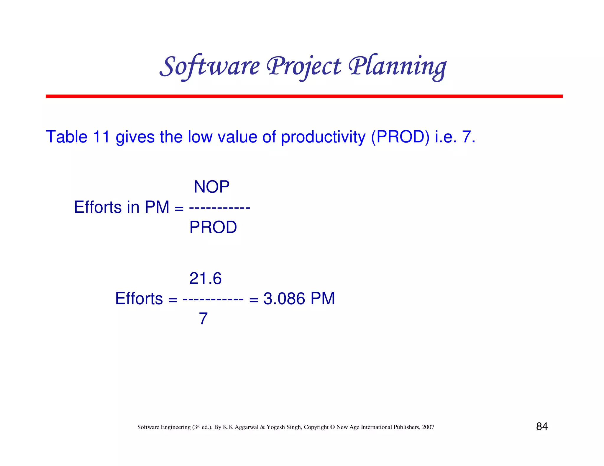
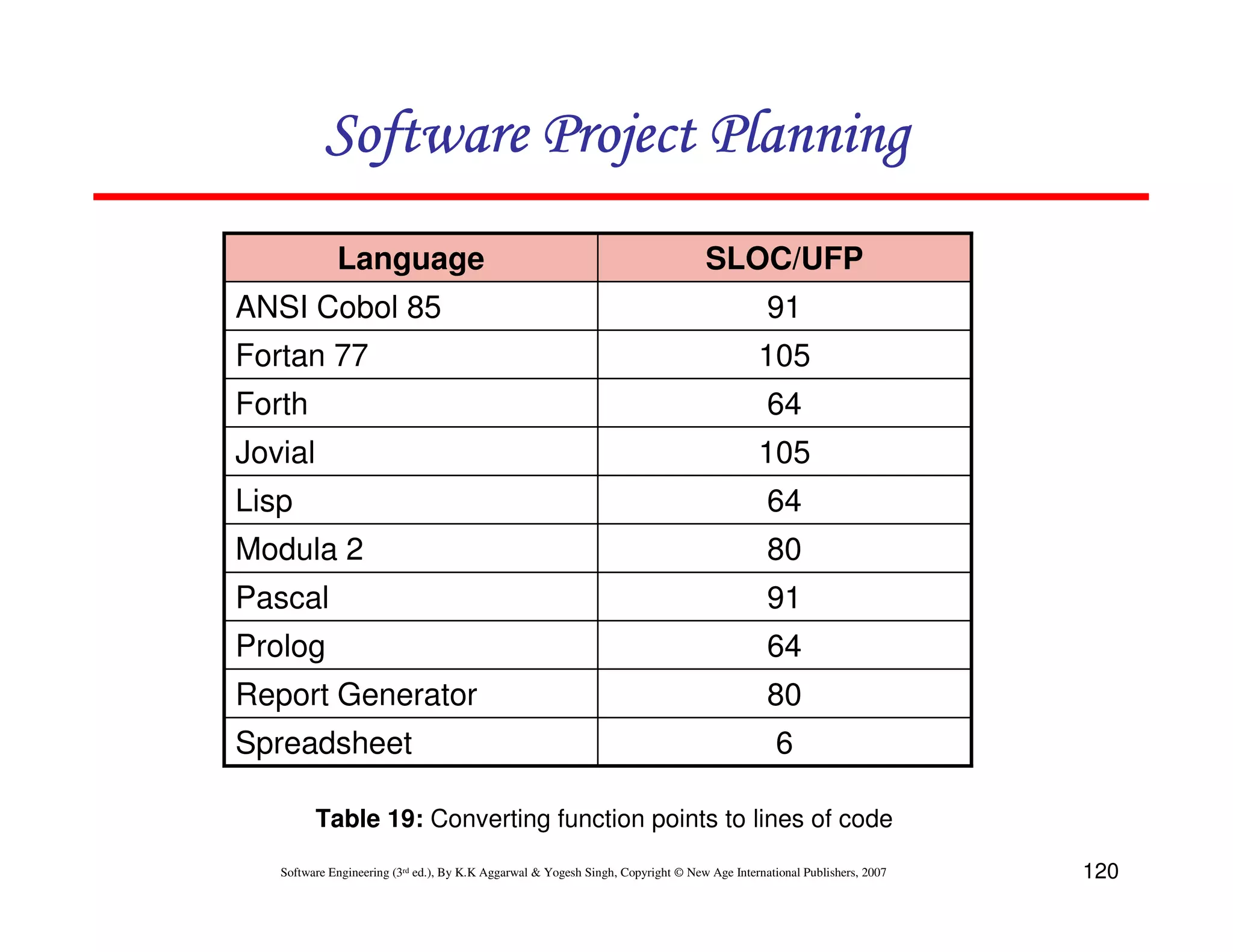
The document discusses software project planning and size estimation techniques. It describes estimating the size of a software project using lines of code counting, function point analysis, and examples. Function point analysis involves decomposing a system into functional units like inputs, outputs, files and inquiries. Each unit is assigned a complexity weight and counted. The weighted counts are summed to calculate unadjusted function points. Adjustments are then made based on complexity factors to determine the final function point count, which can be used to estimate effort, cost and schedule for a project. Three examples are provided to illustrate calculating function points for sample projects.
Introduction to Software Engineering by K.K Aggarwal & Yogesh Singh.
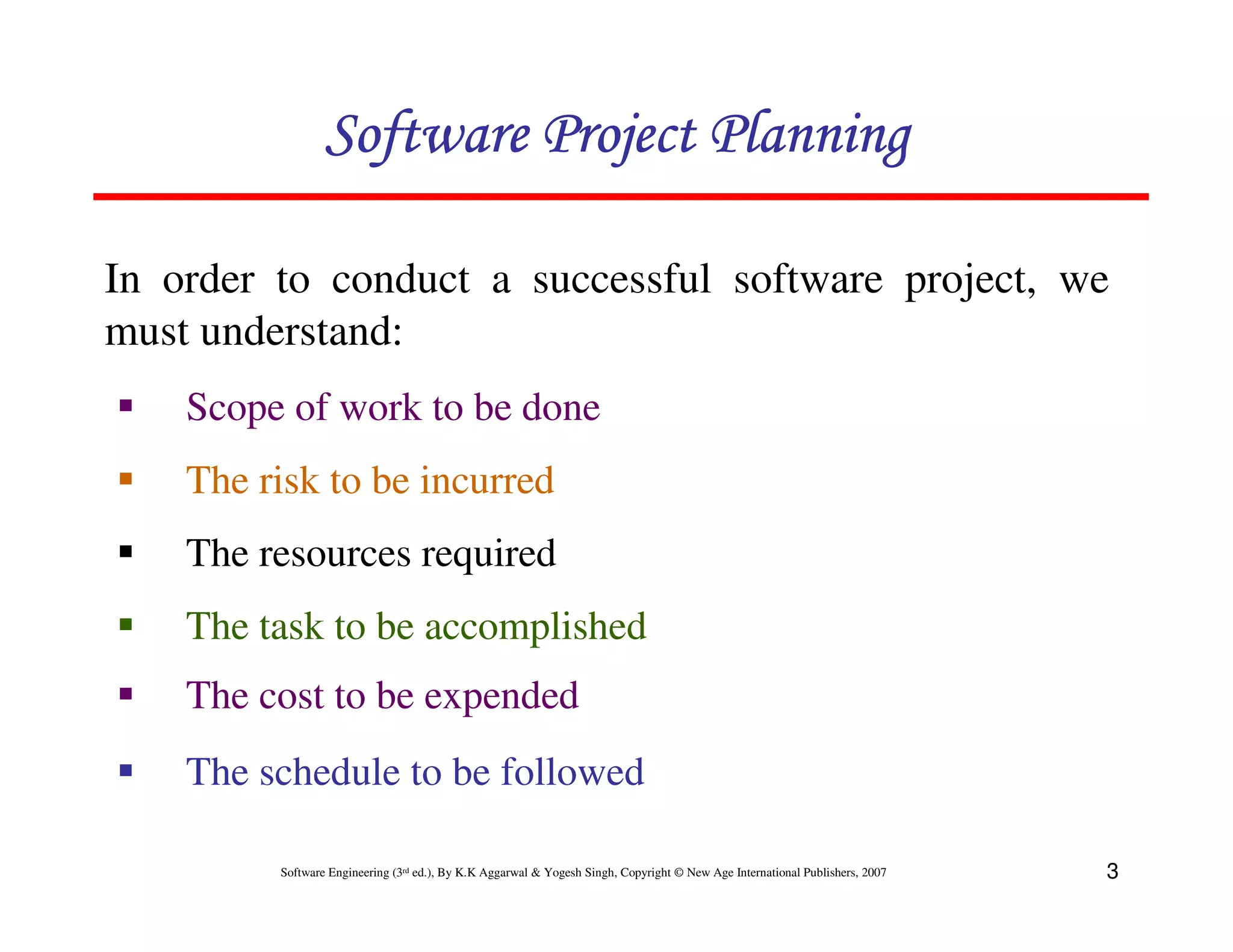
Covers size, cost, and time estimation; Importance of understanding work scope, risks, resources, tasks, costs, and schedules.
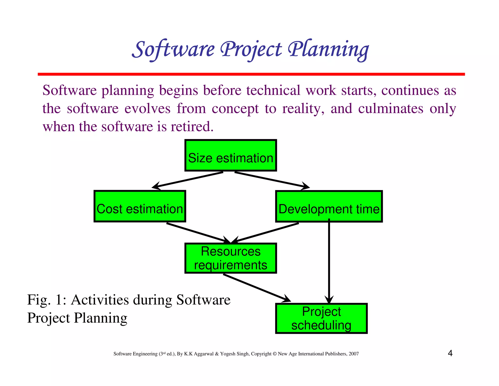
Planning activities vary throughout project lifecycle; Importance of size, cost, development time, resources, and scheduling.
Discusses Lines of Code (LOC) as a size estimation metric, including definitions of comments and code; covers discrepancies and Conte's definition.
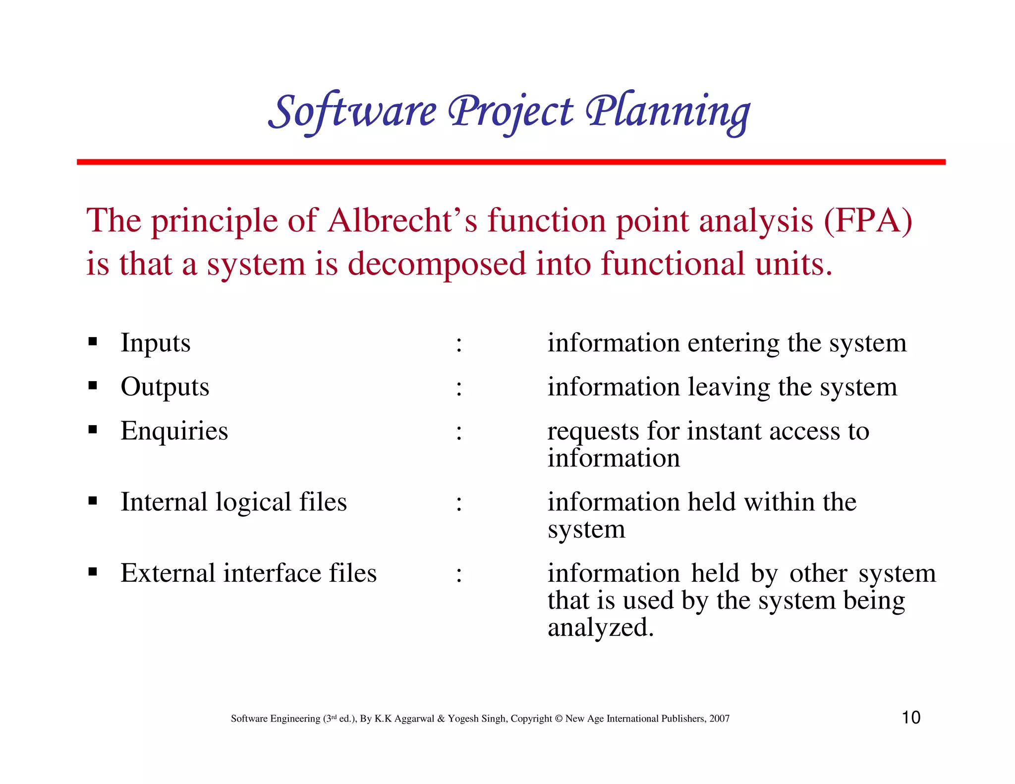
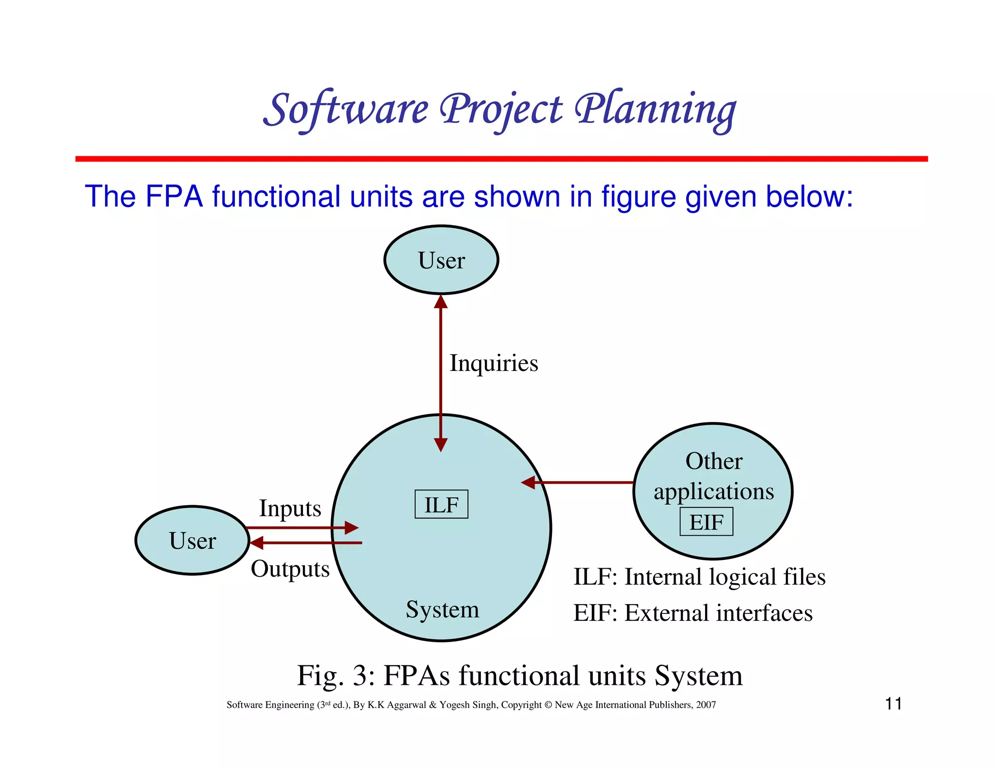
Introduces Function Point Analysis (FPA) for measuring software size using functional units like inputs, outputs, and inquiries.
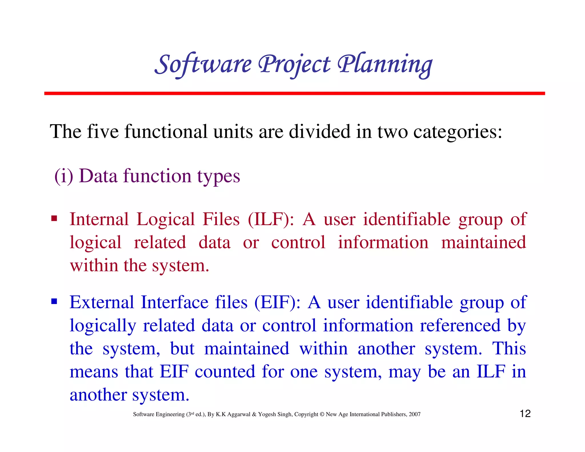
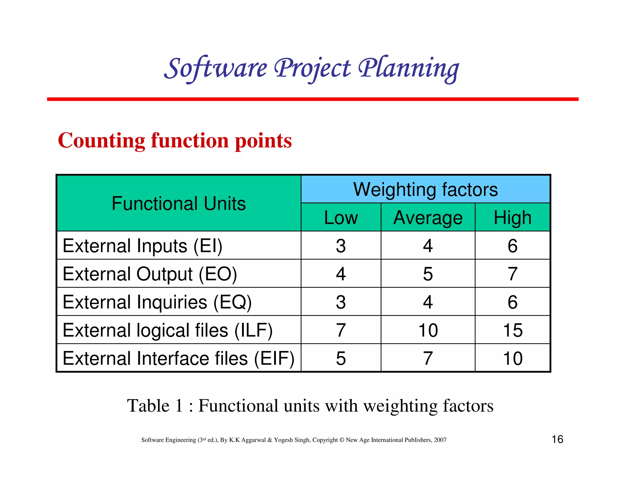
Defines unit types in FPA and how to calculate unadjusted function points (UFP) using complexity and weighting factors.
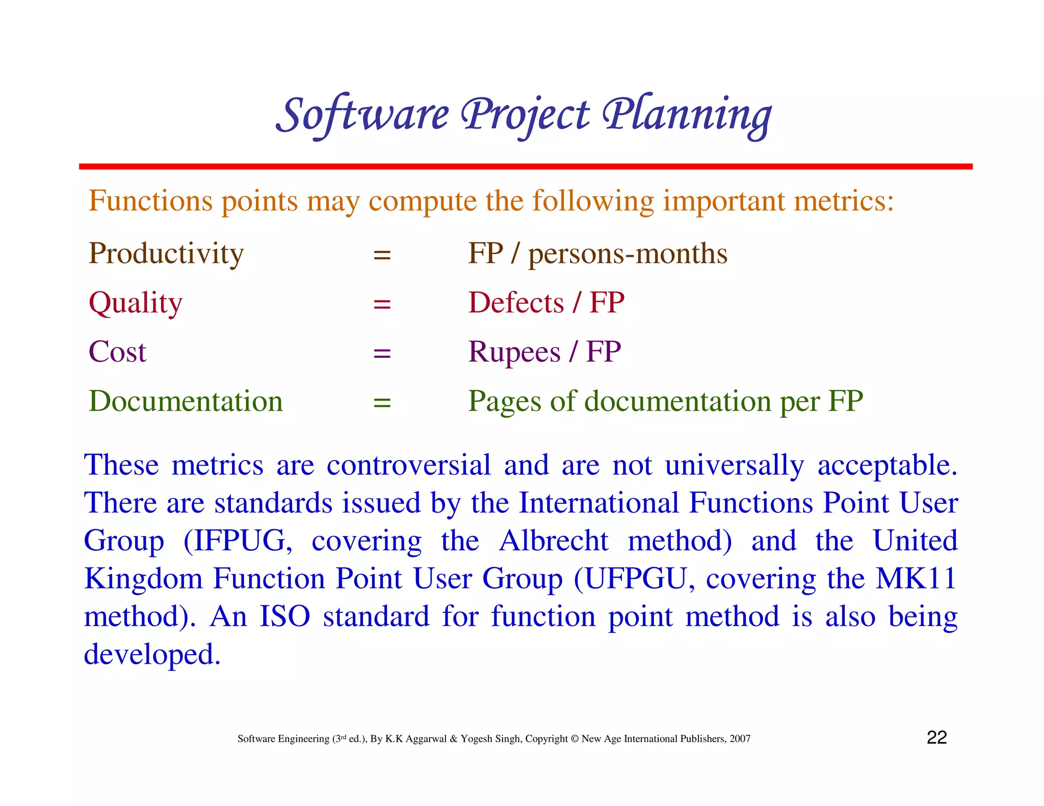
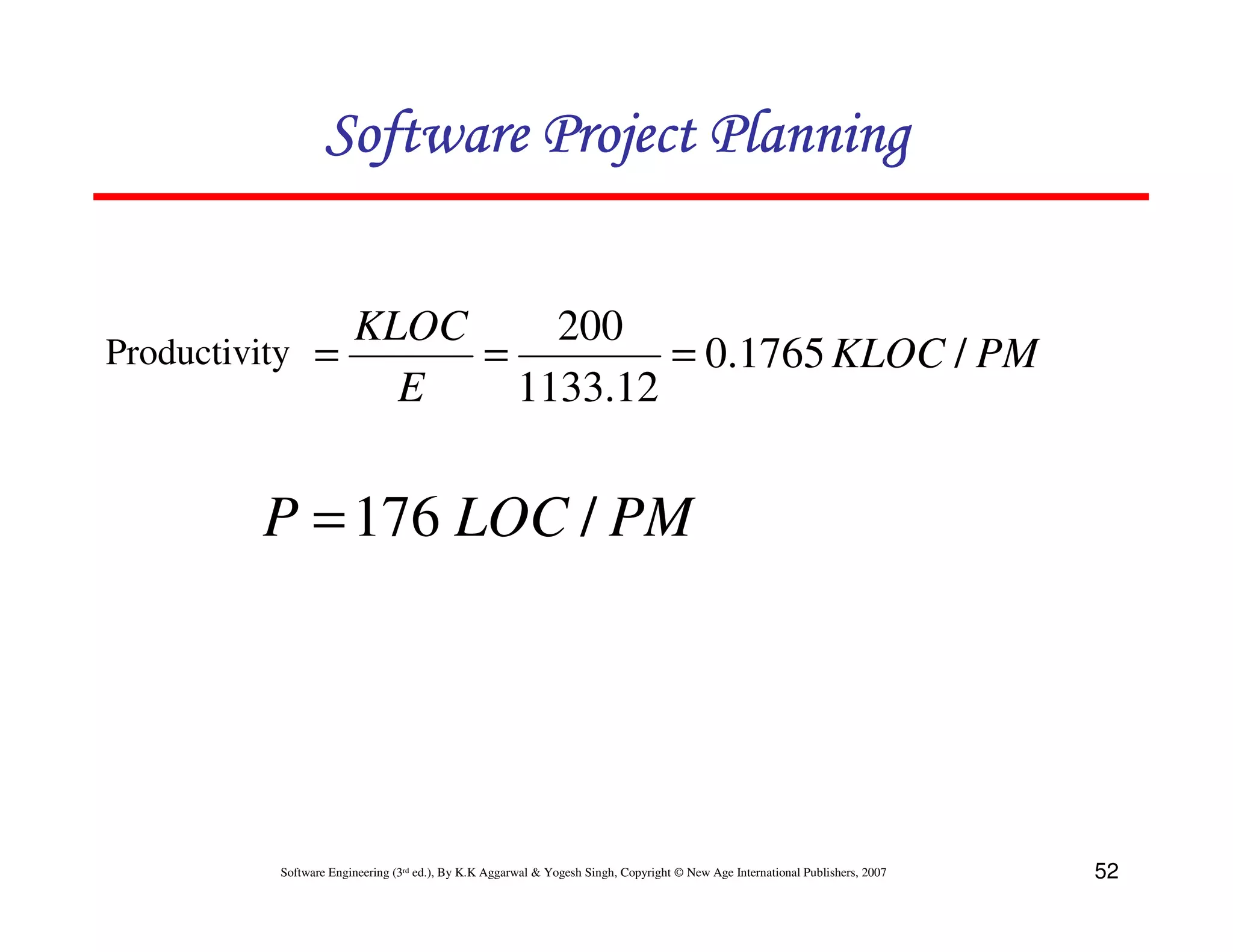
Discusses metrics derived from function points including quality, productivity, cost, and documentation.
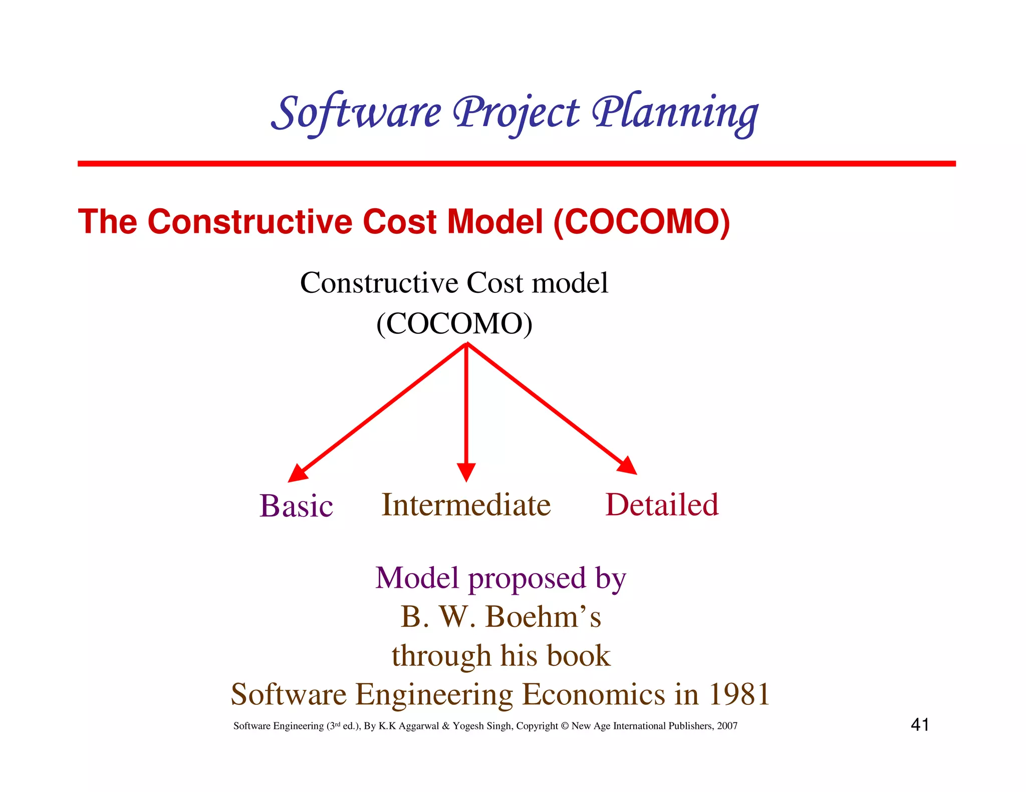
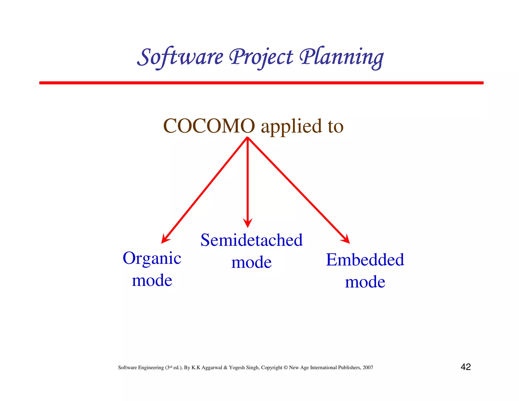
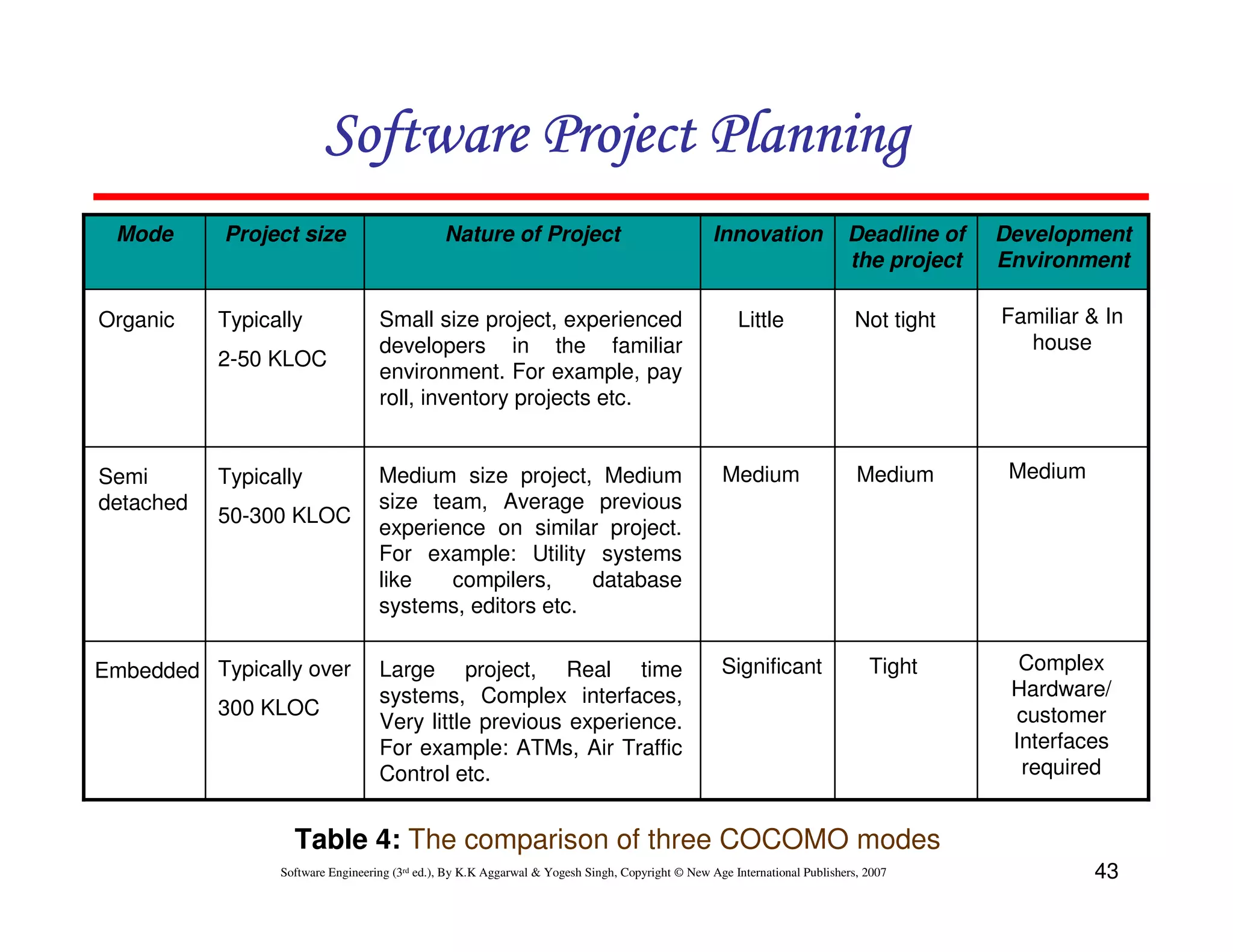
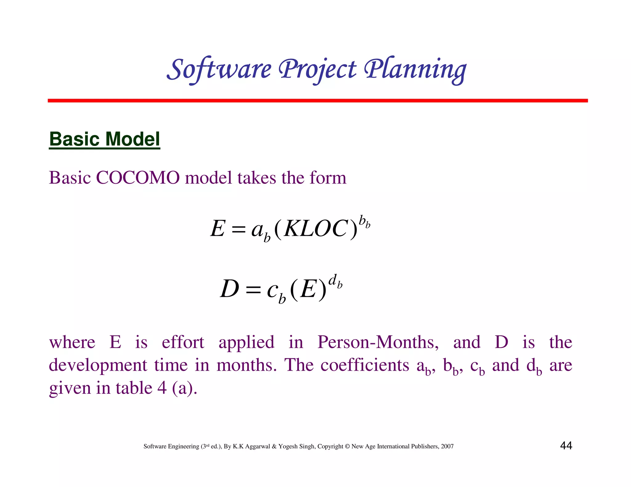
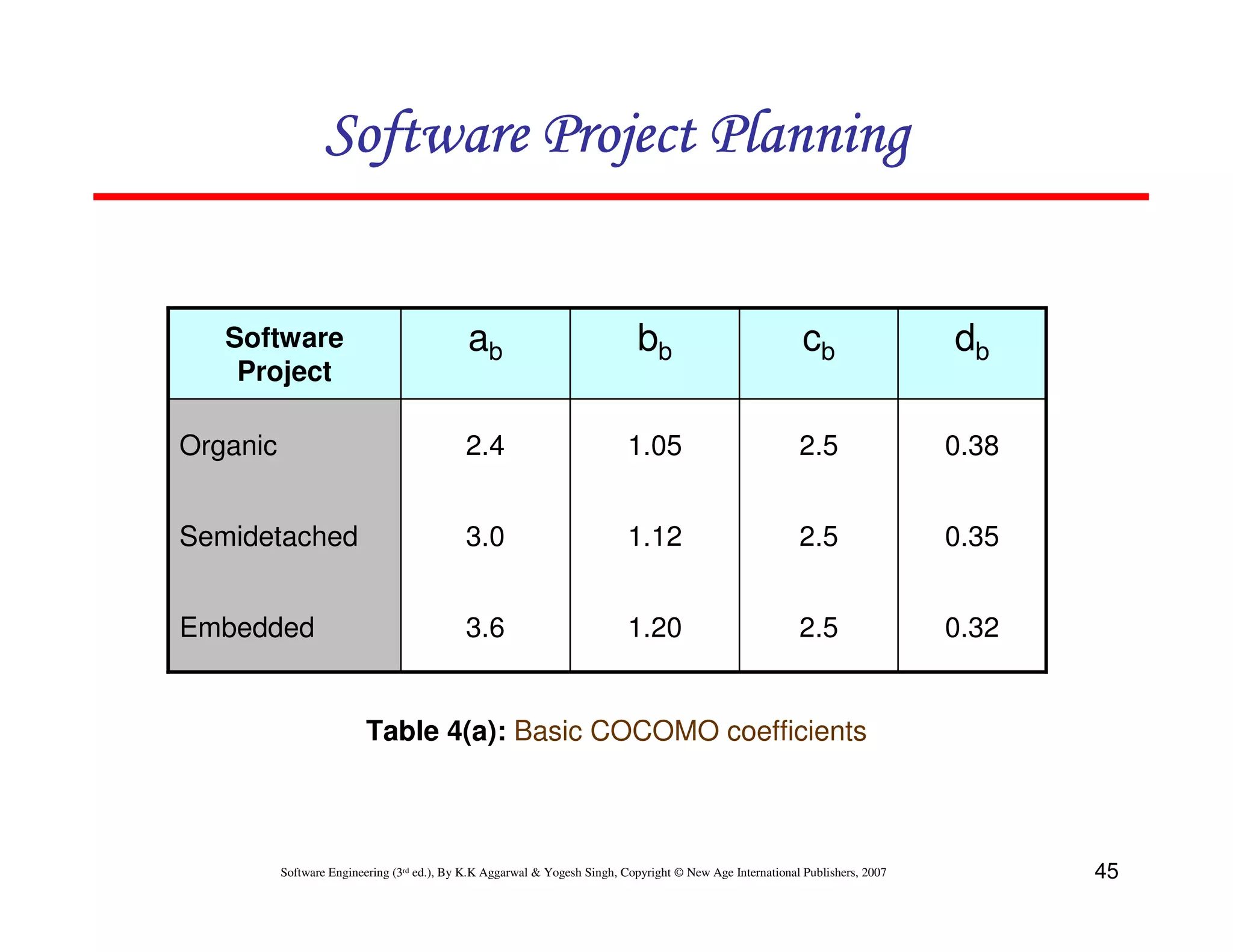
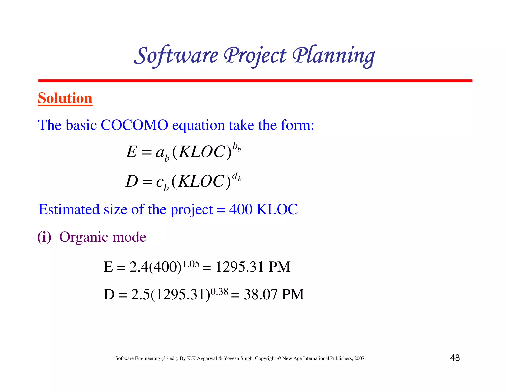
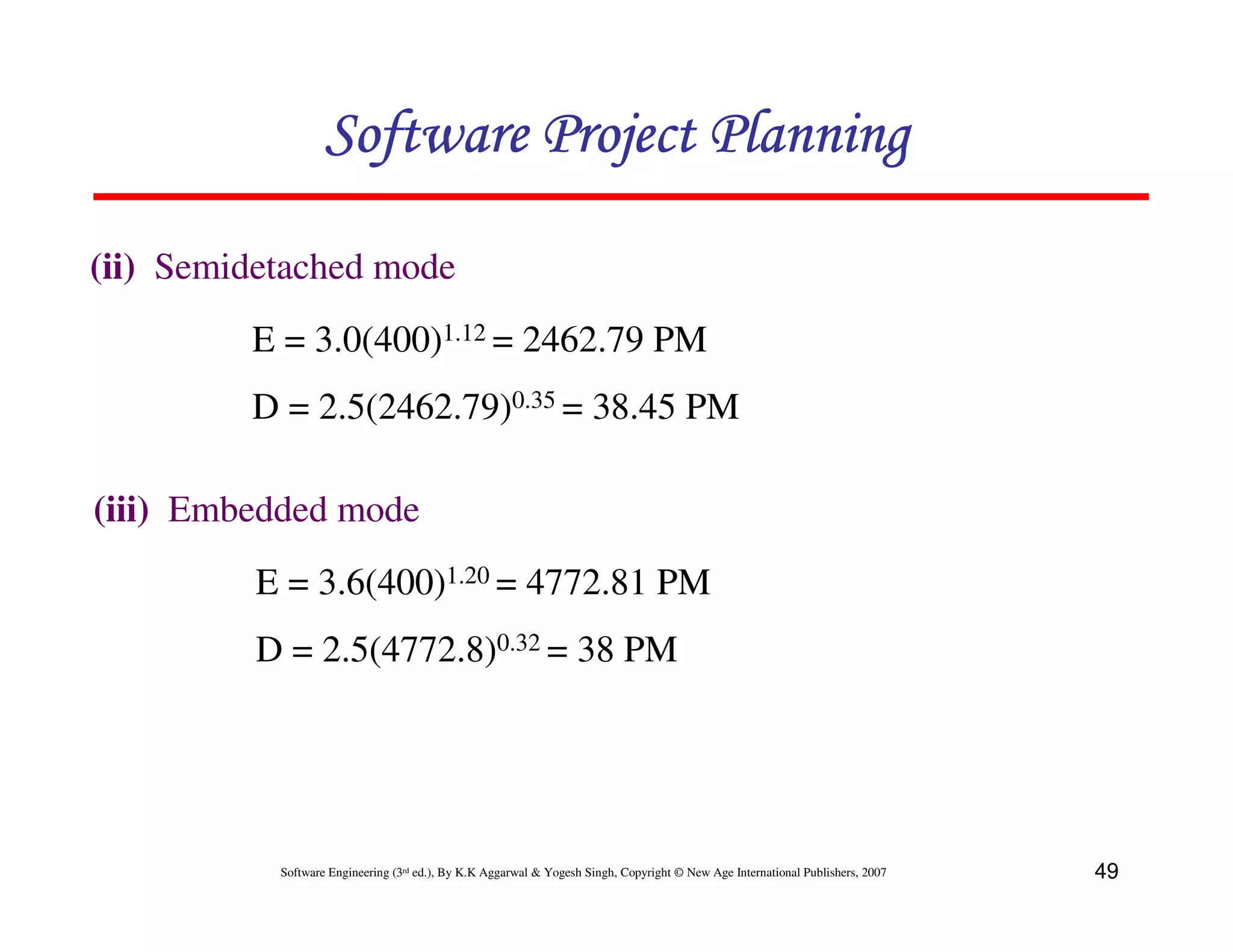
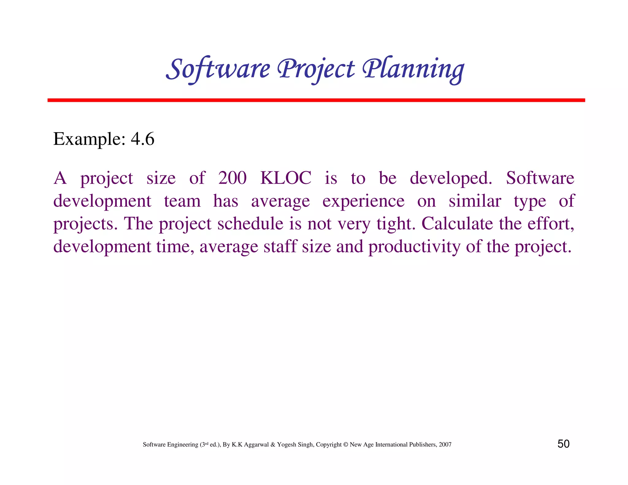
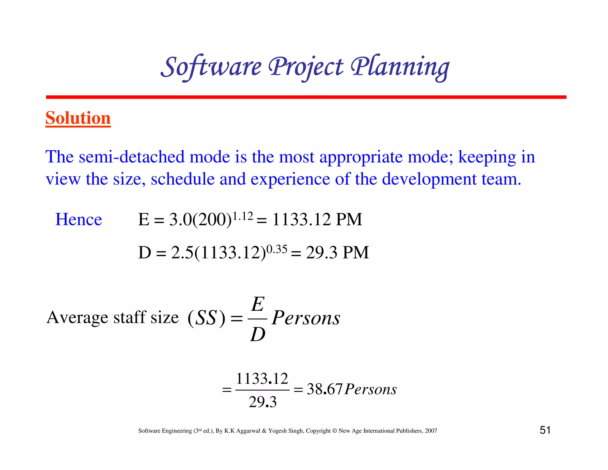
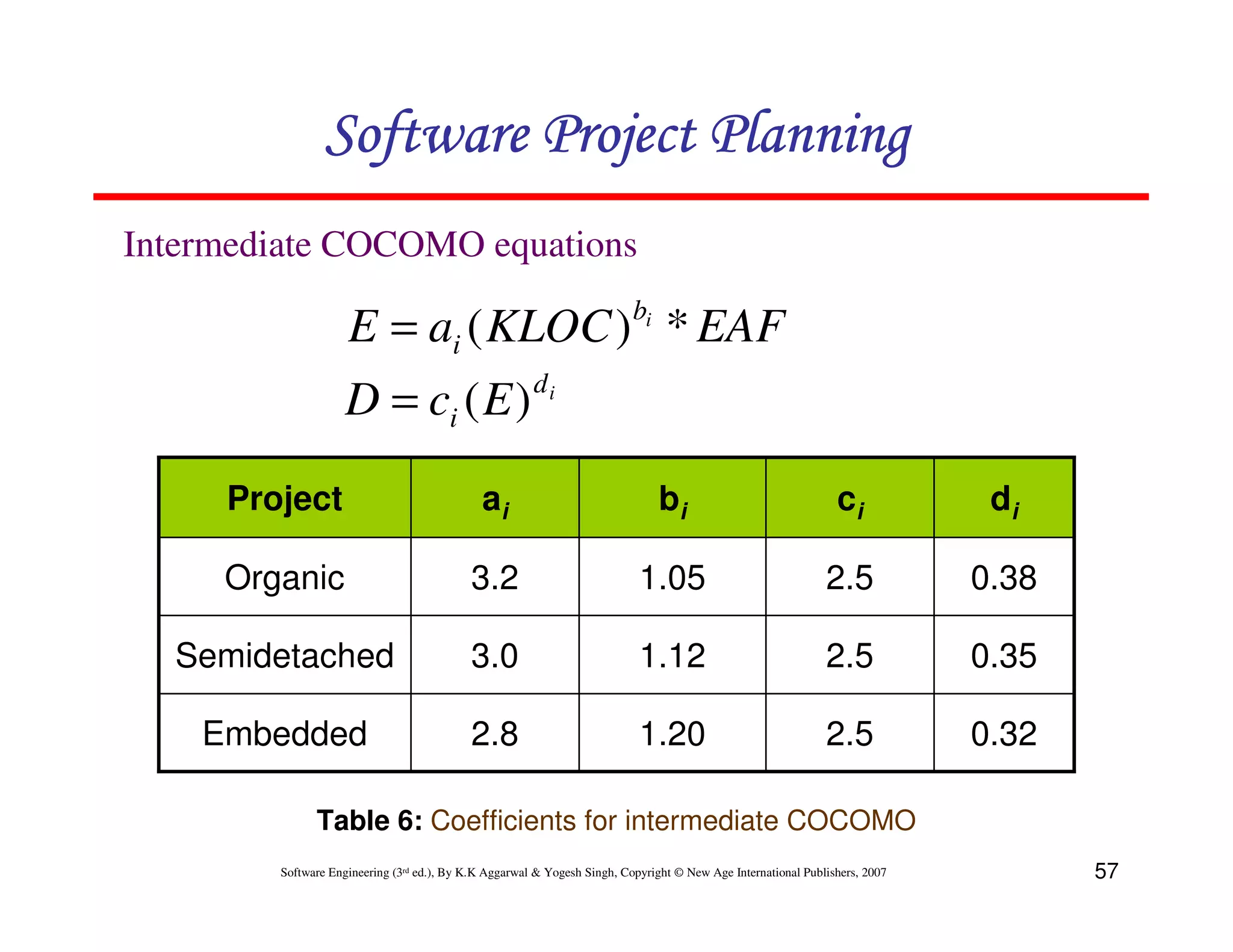
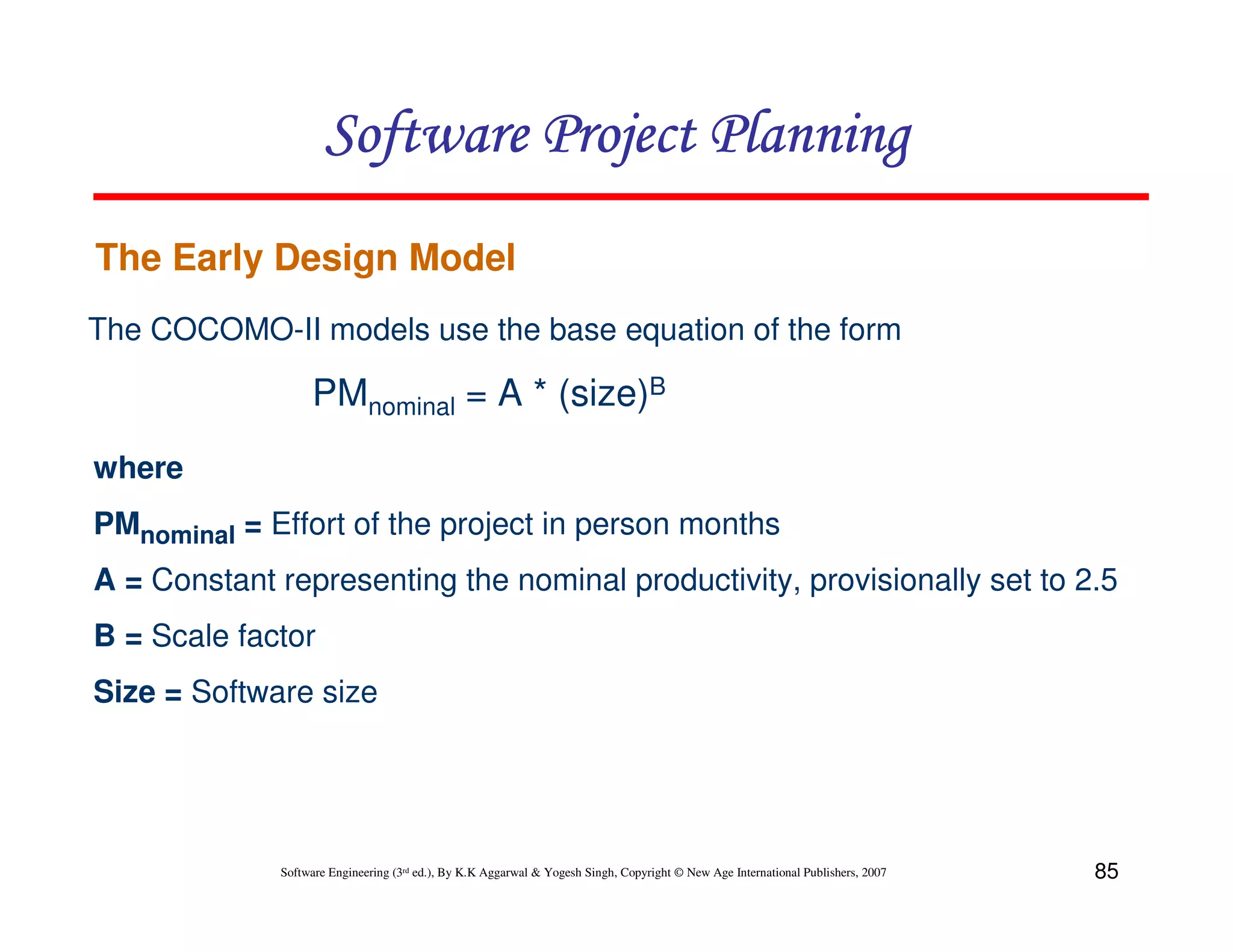
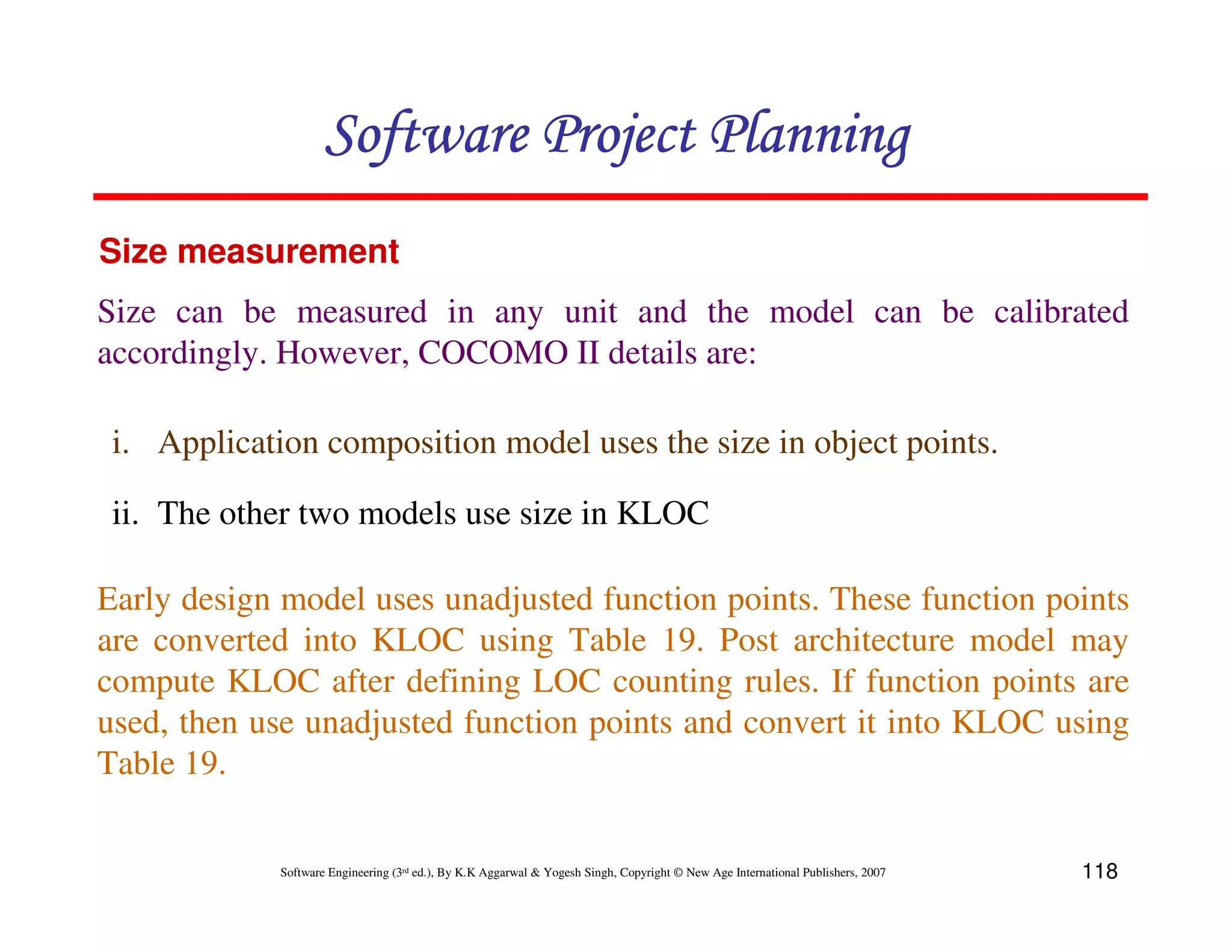
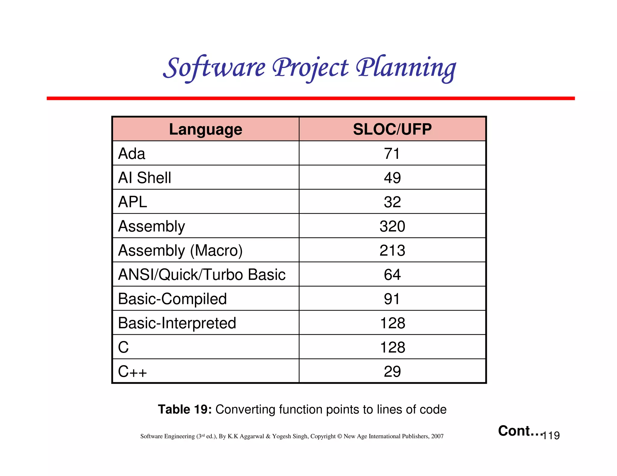
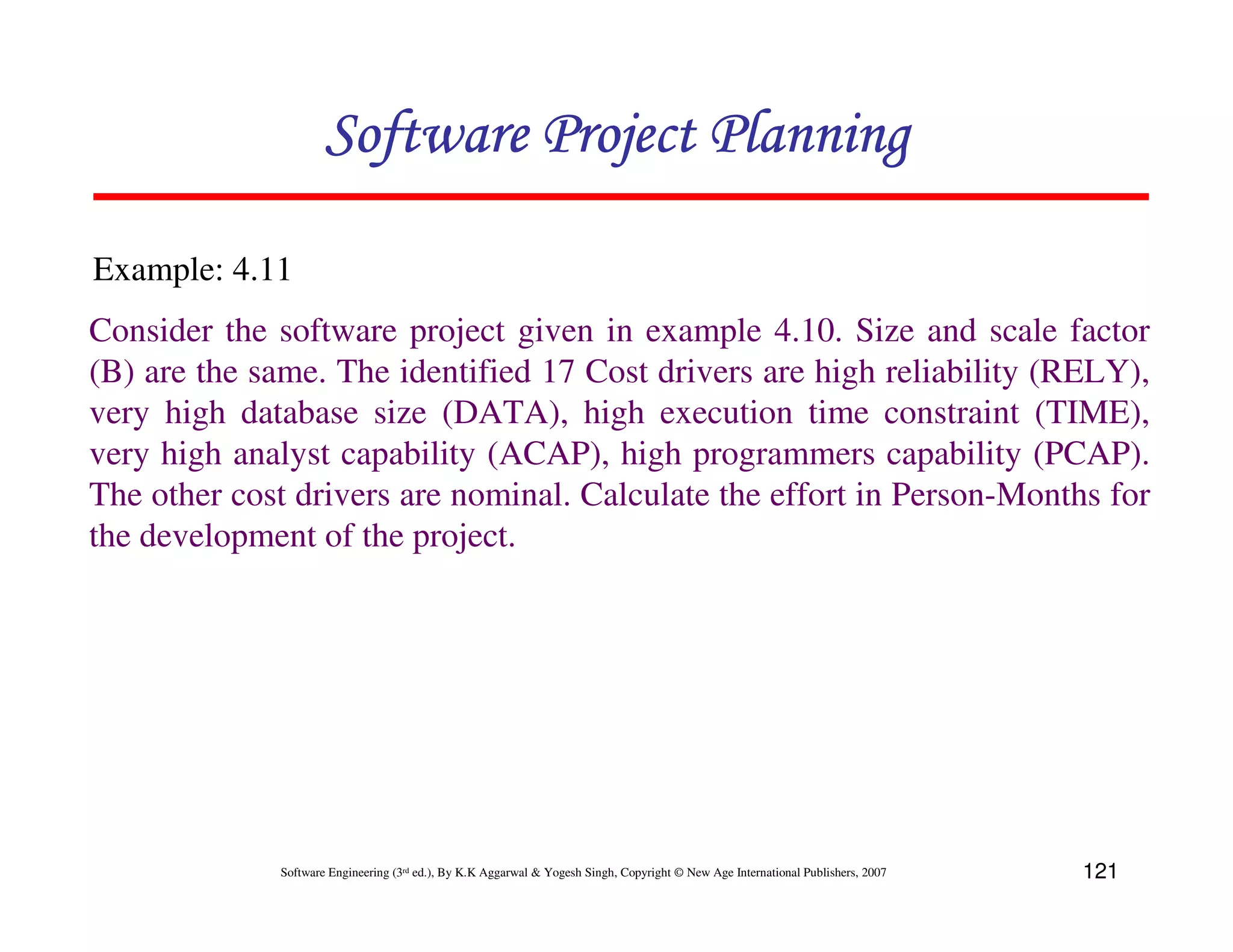
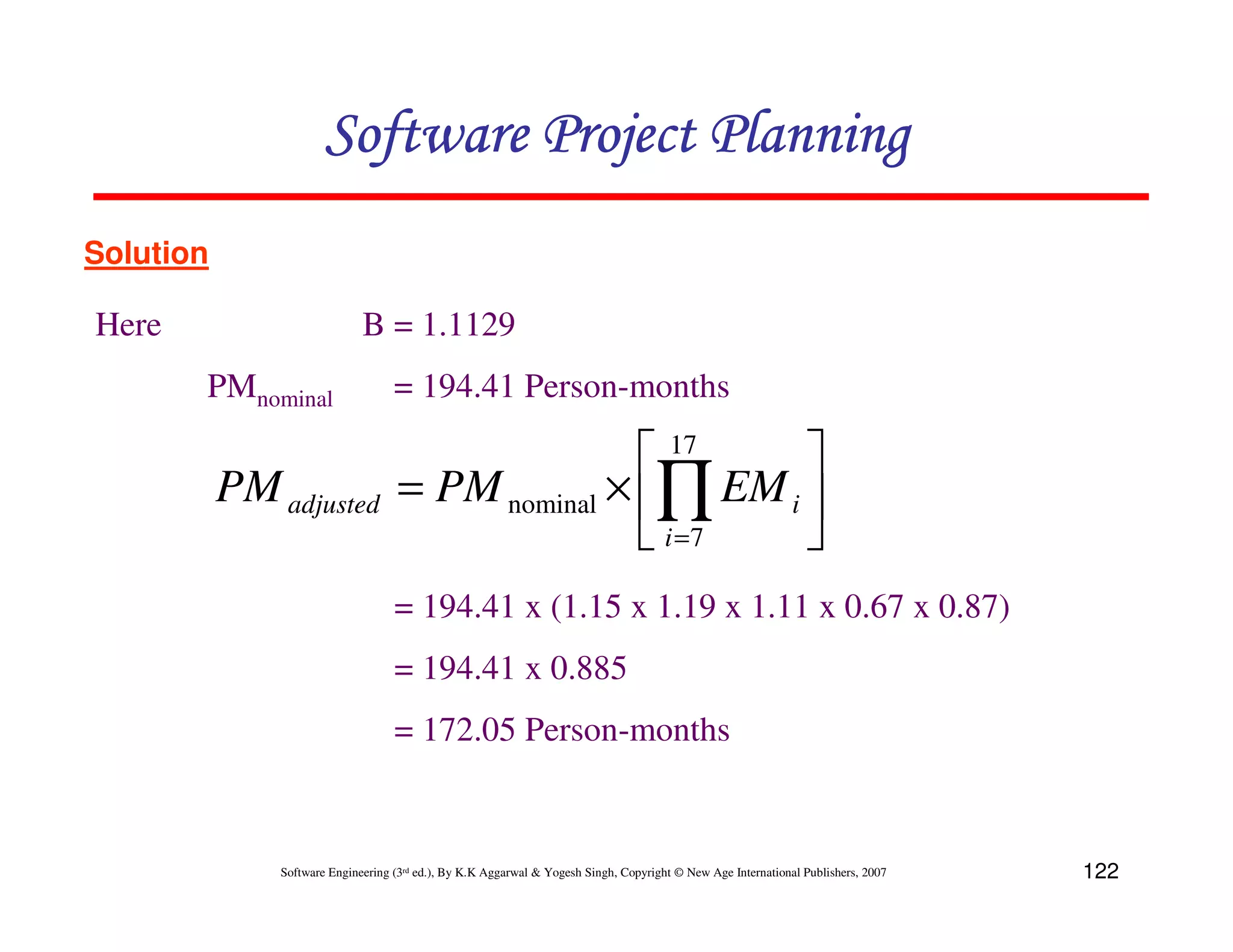
Introduces COCOMO models for estimating software cost and schedule based on project size, describing specific models (Organic, Semidetached, Embedded).
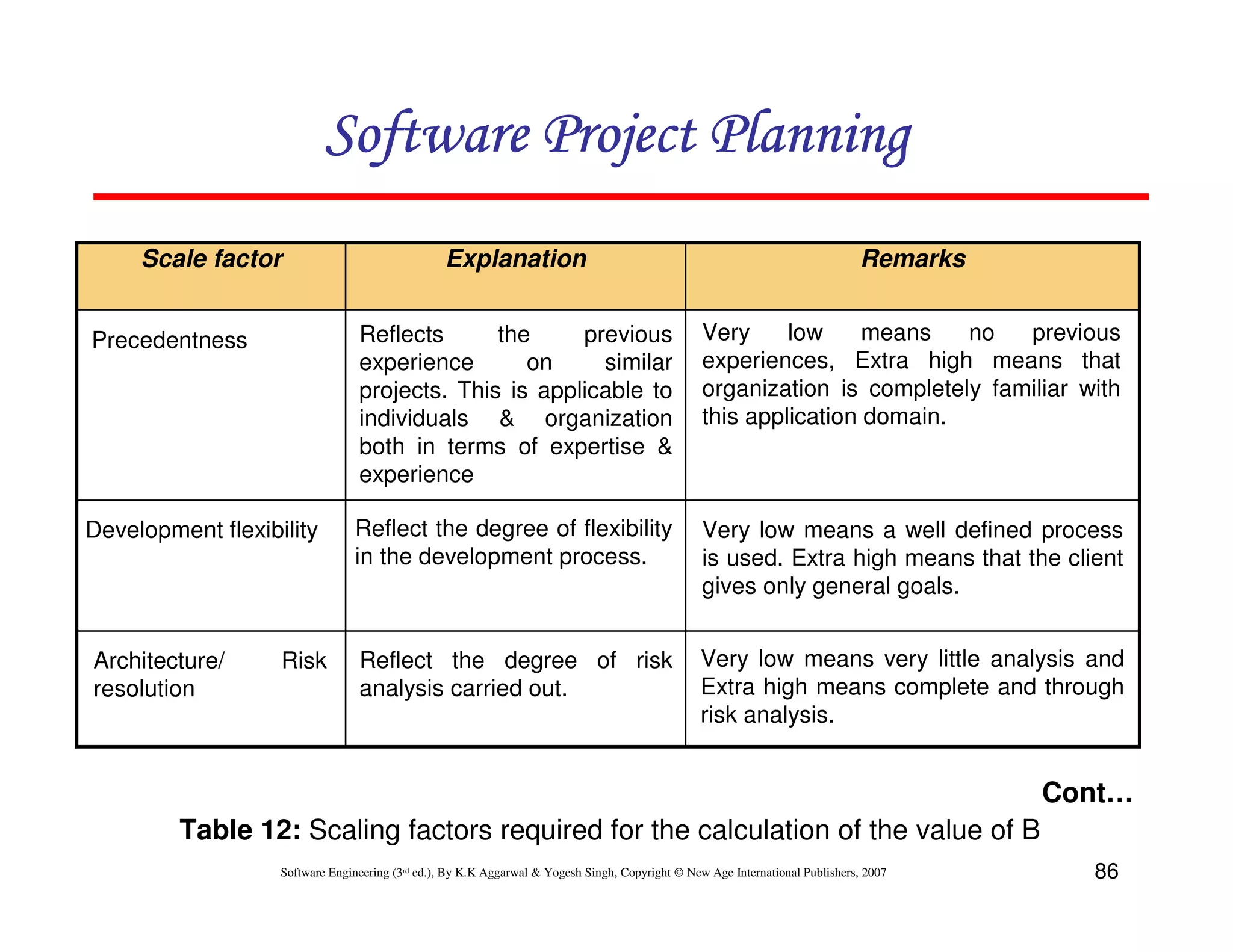
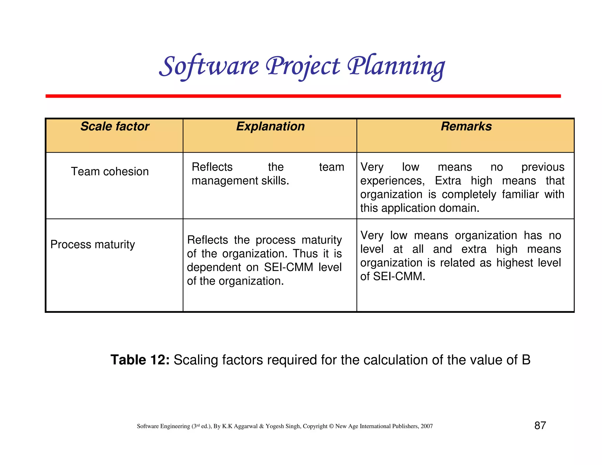
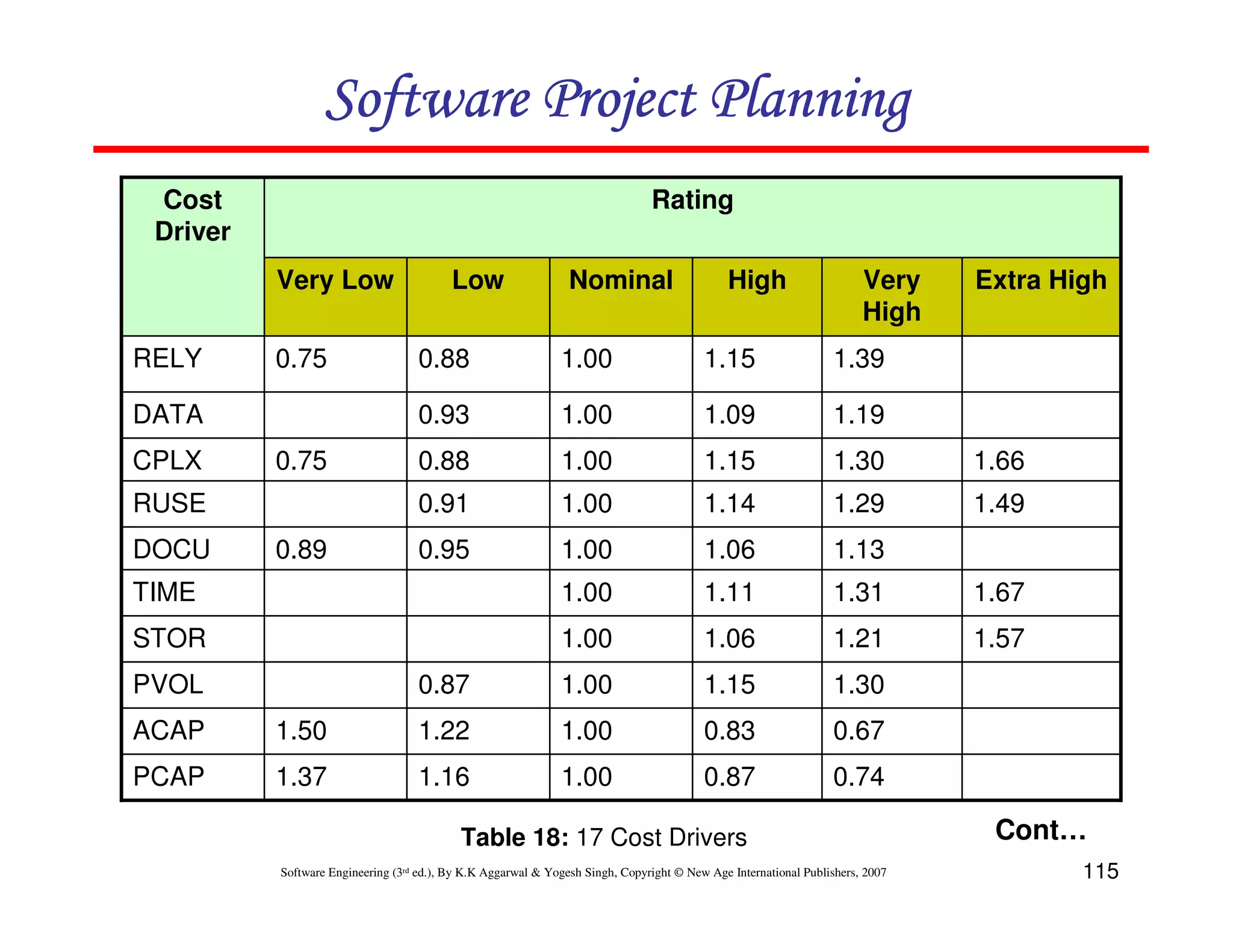
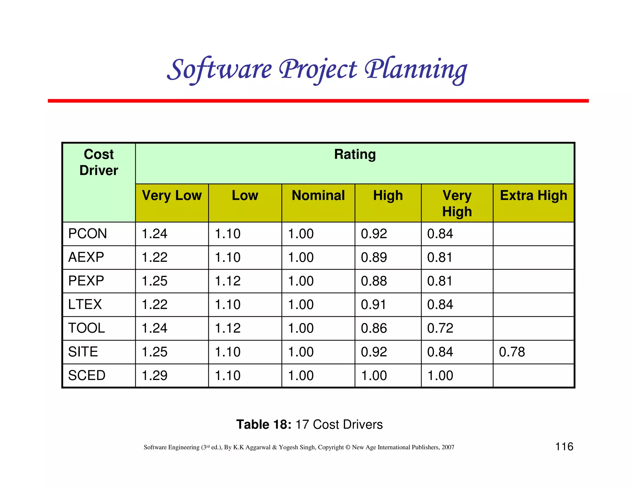
Describes detailed analysis using COCOMO II; Discusses calibration based on cost drivers and environment factors.
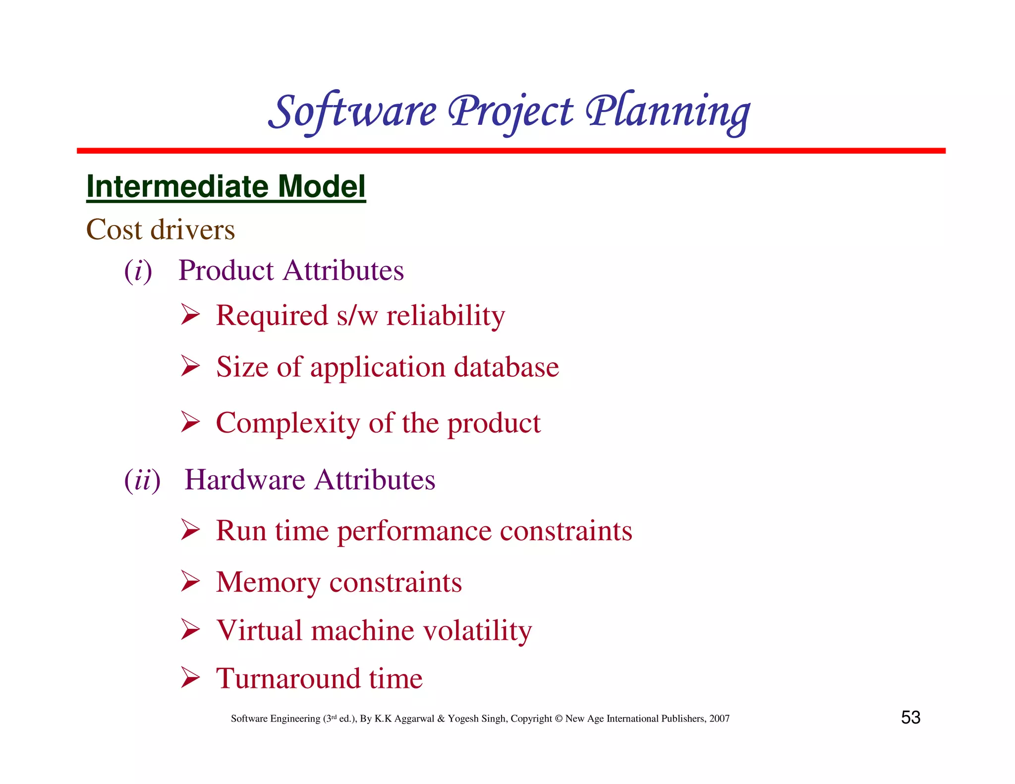
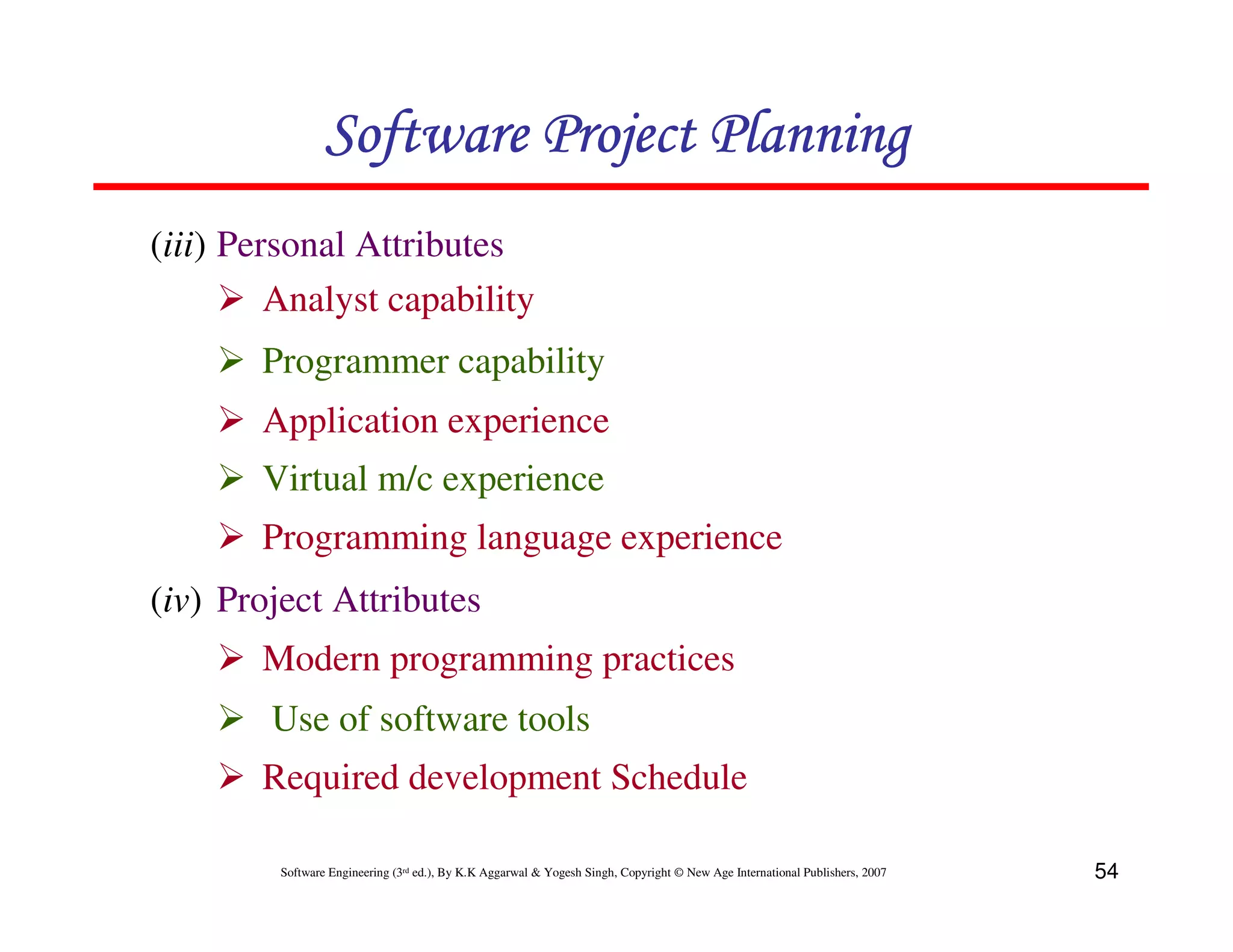
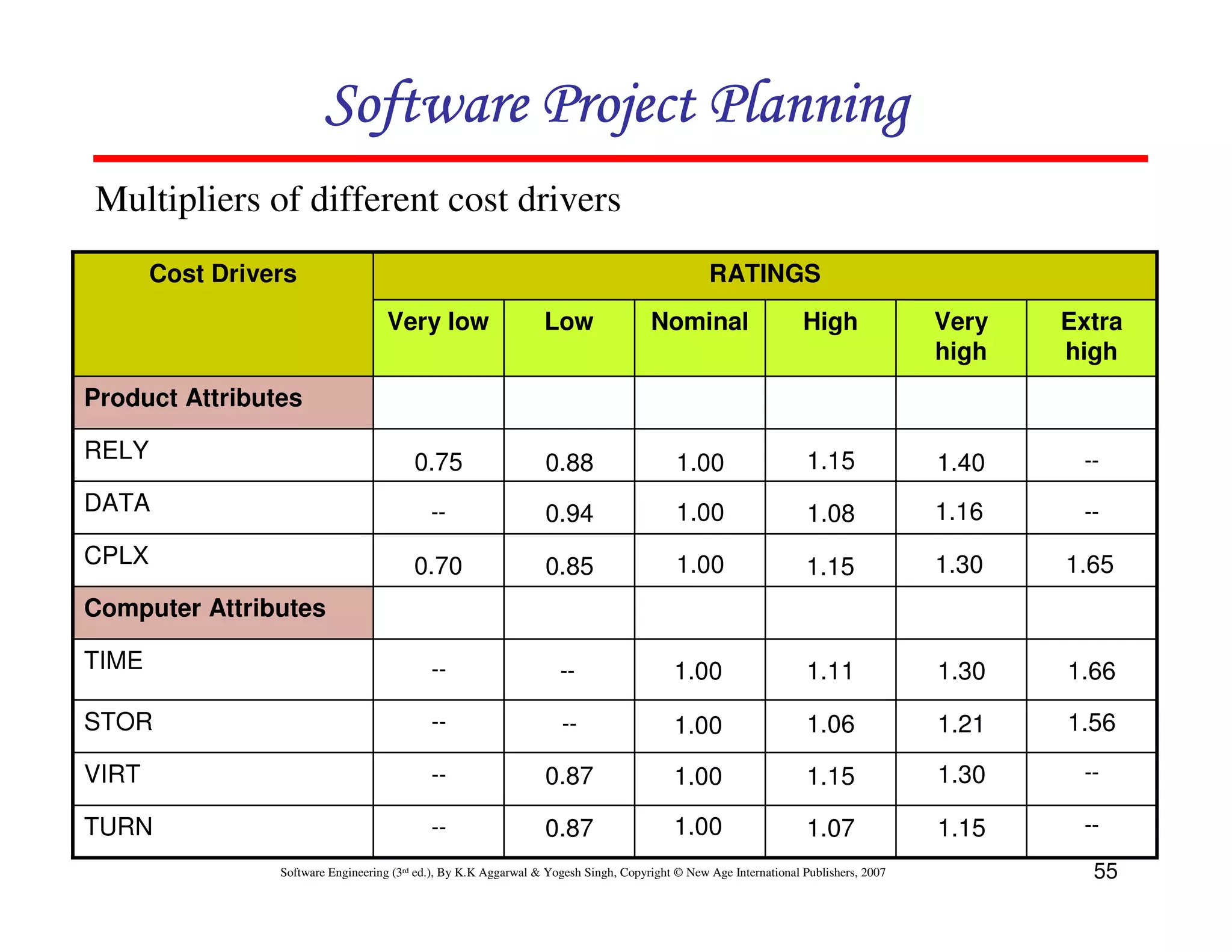
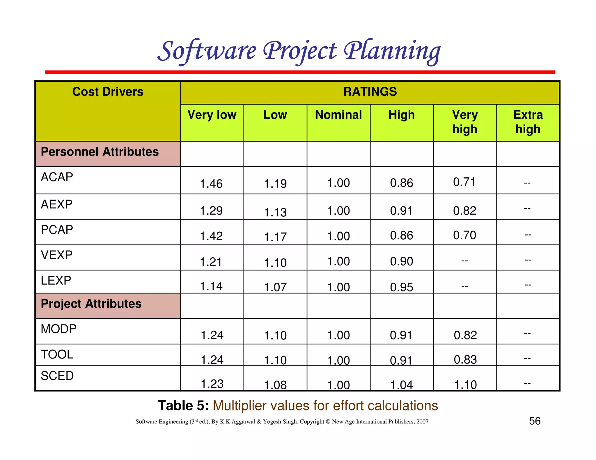
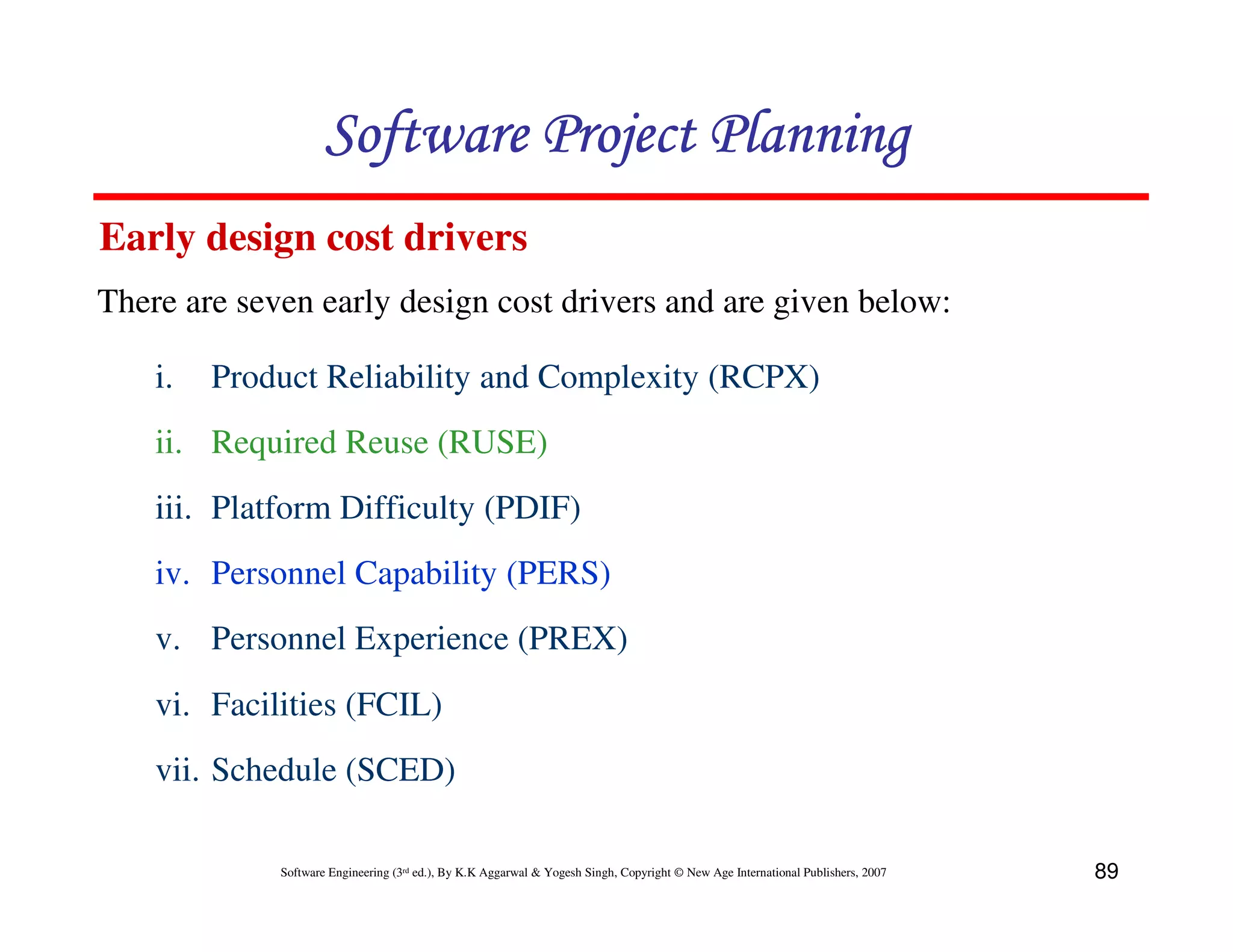
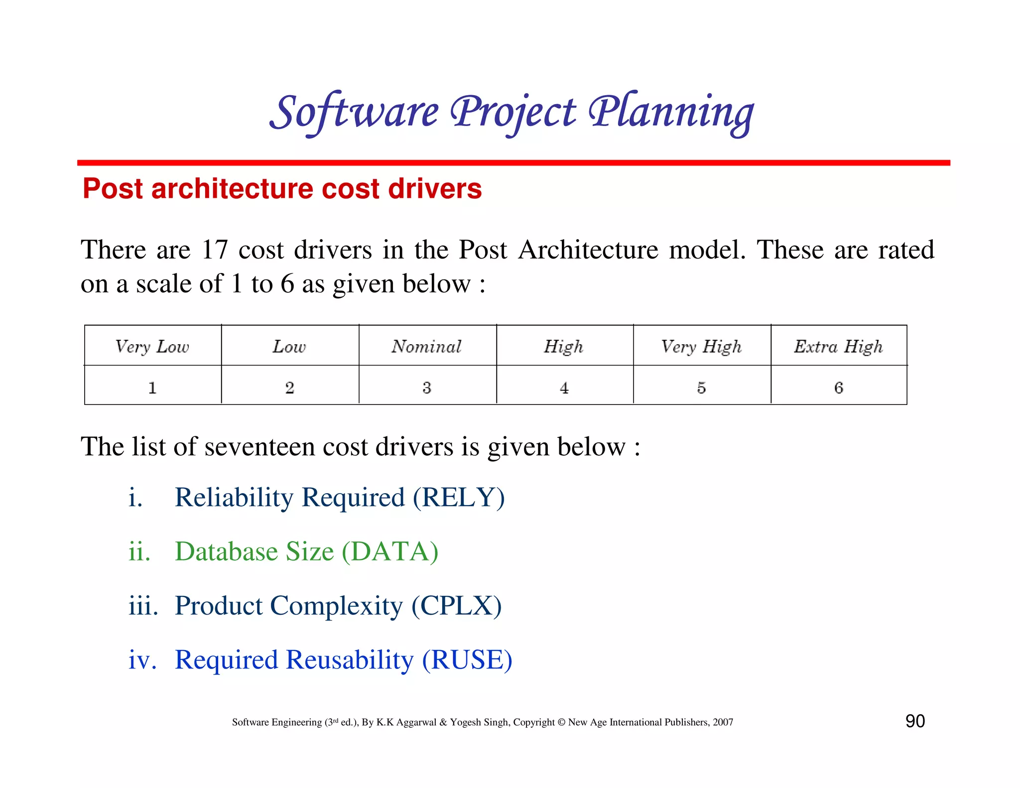
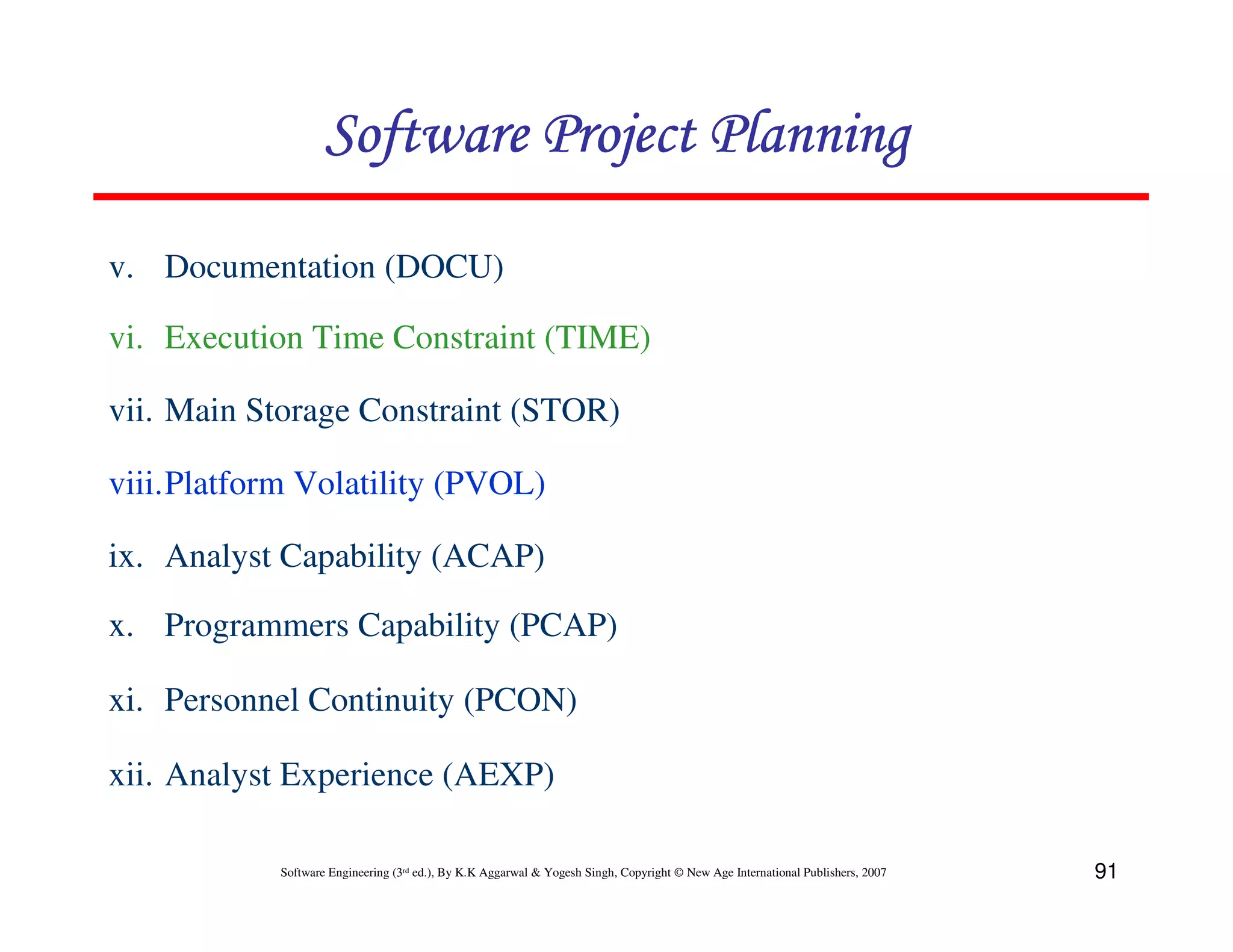
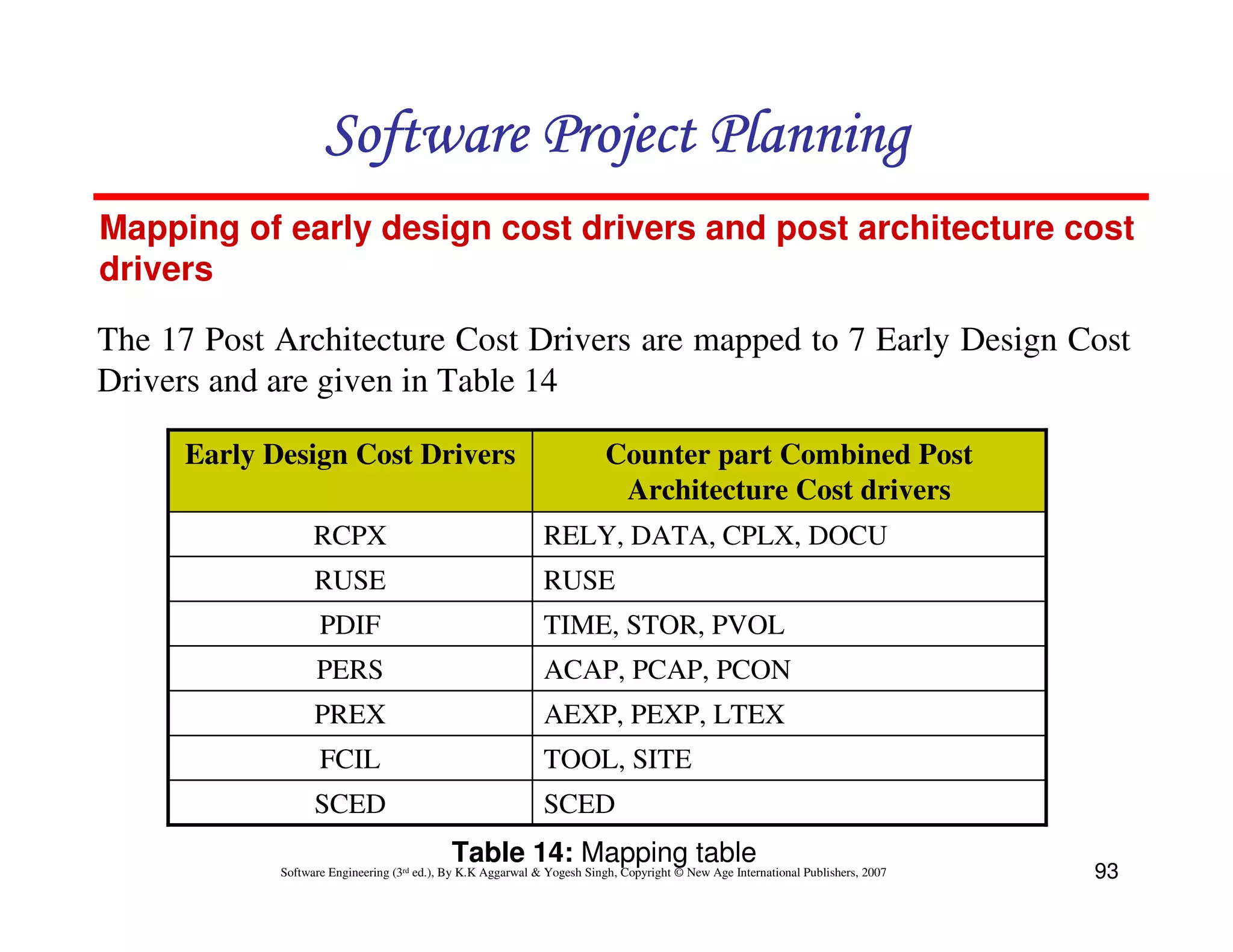
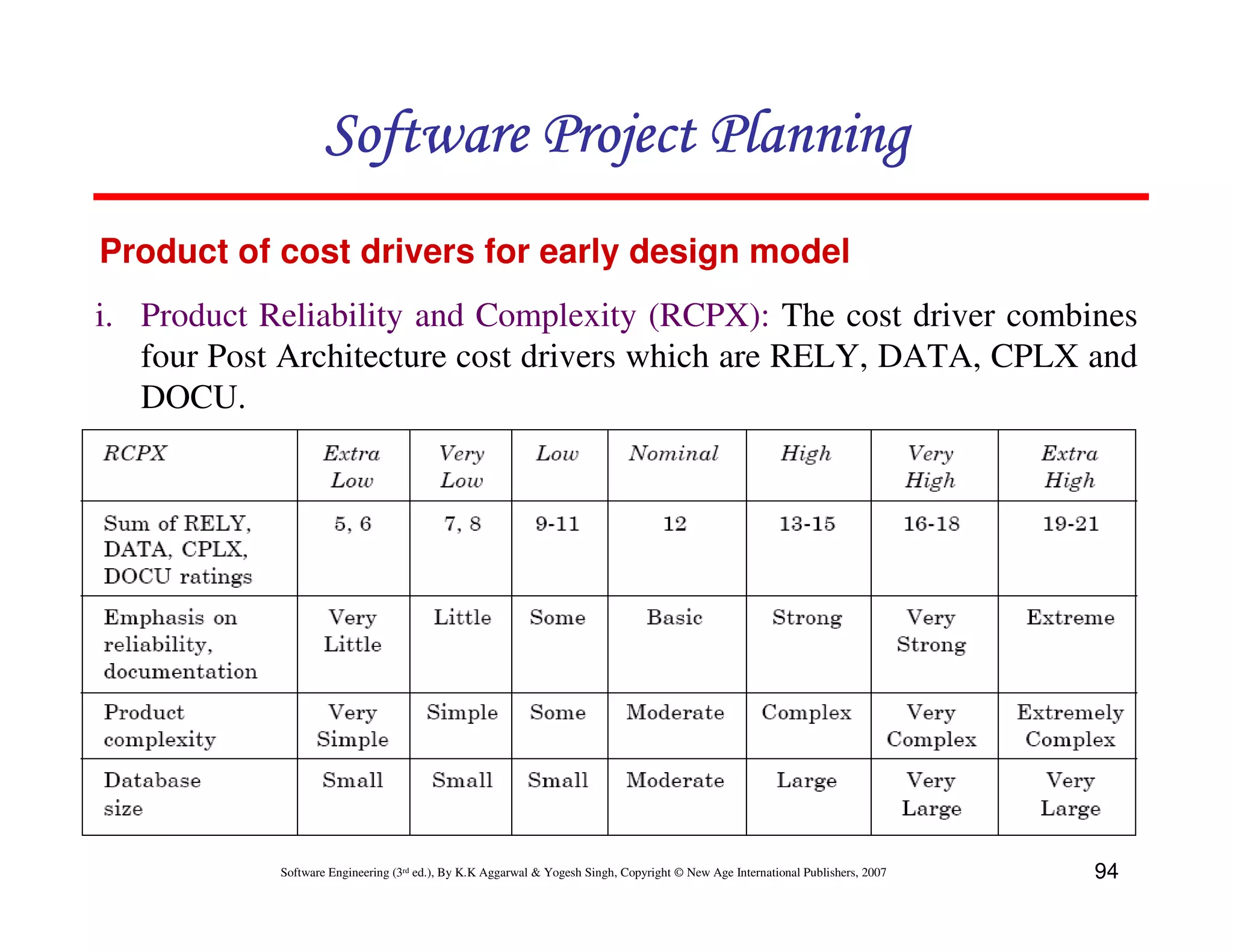
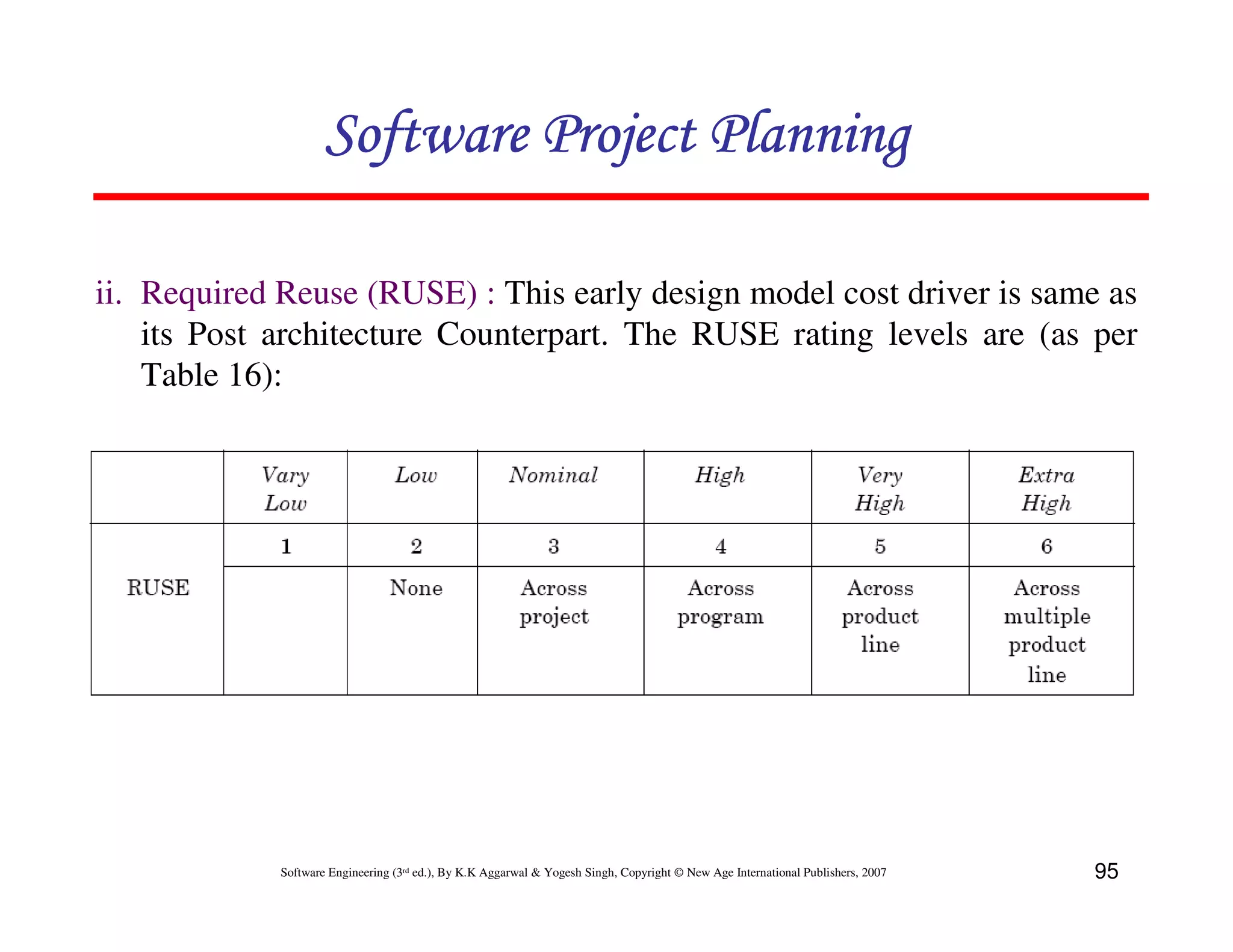
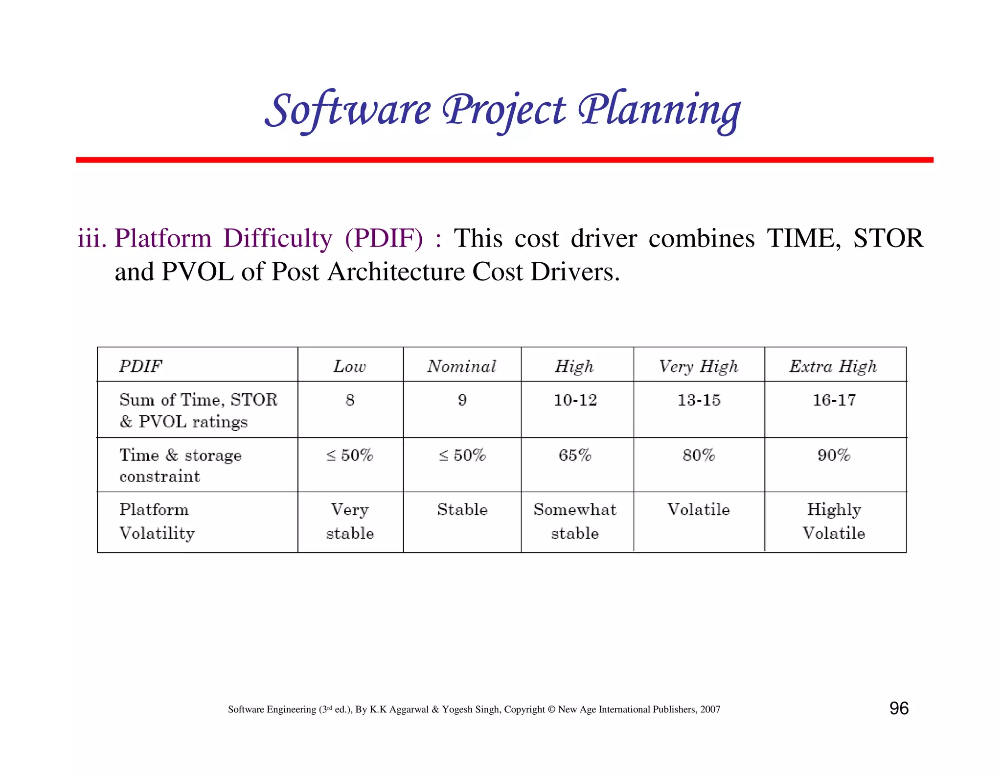
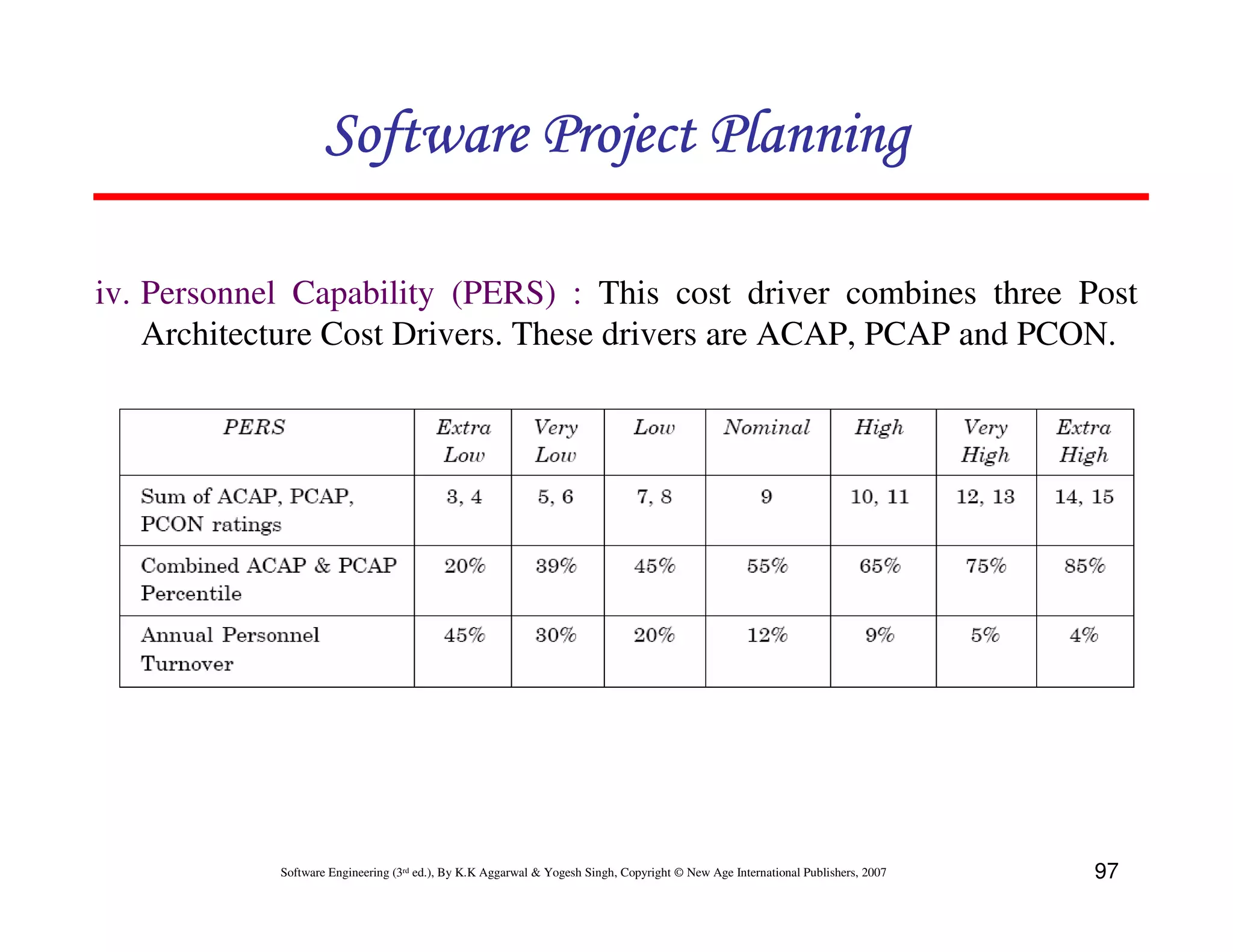
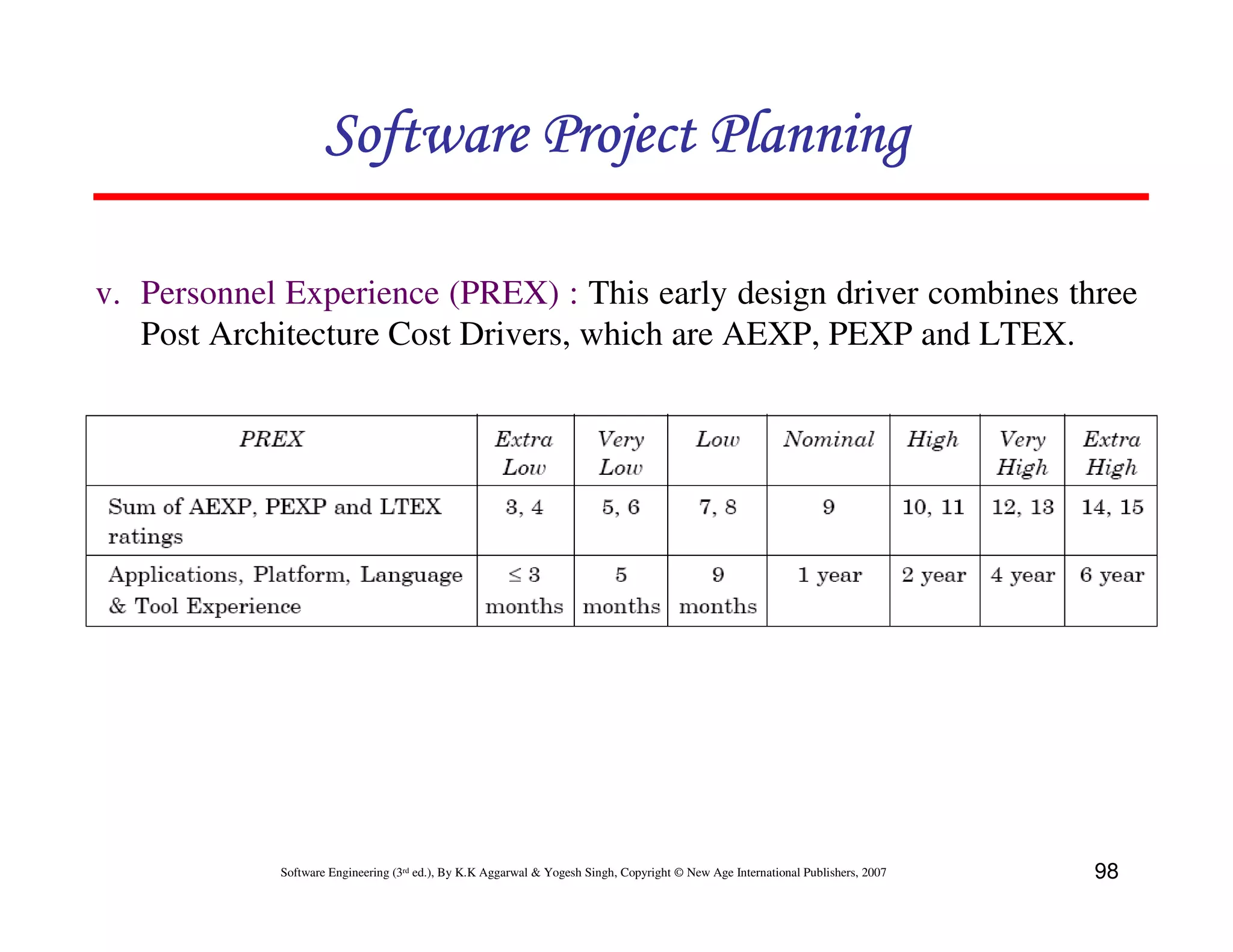
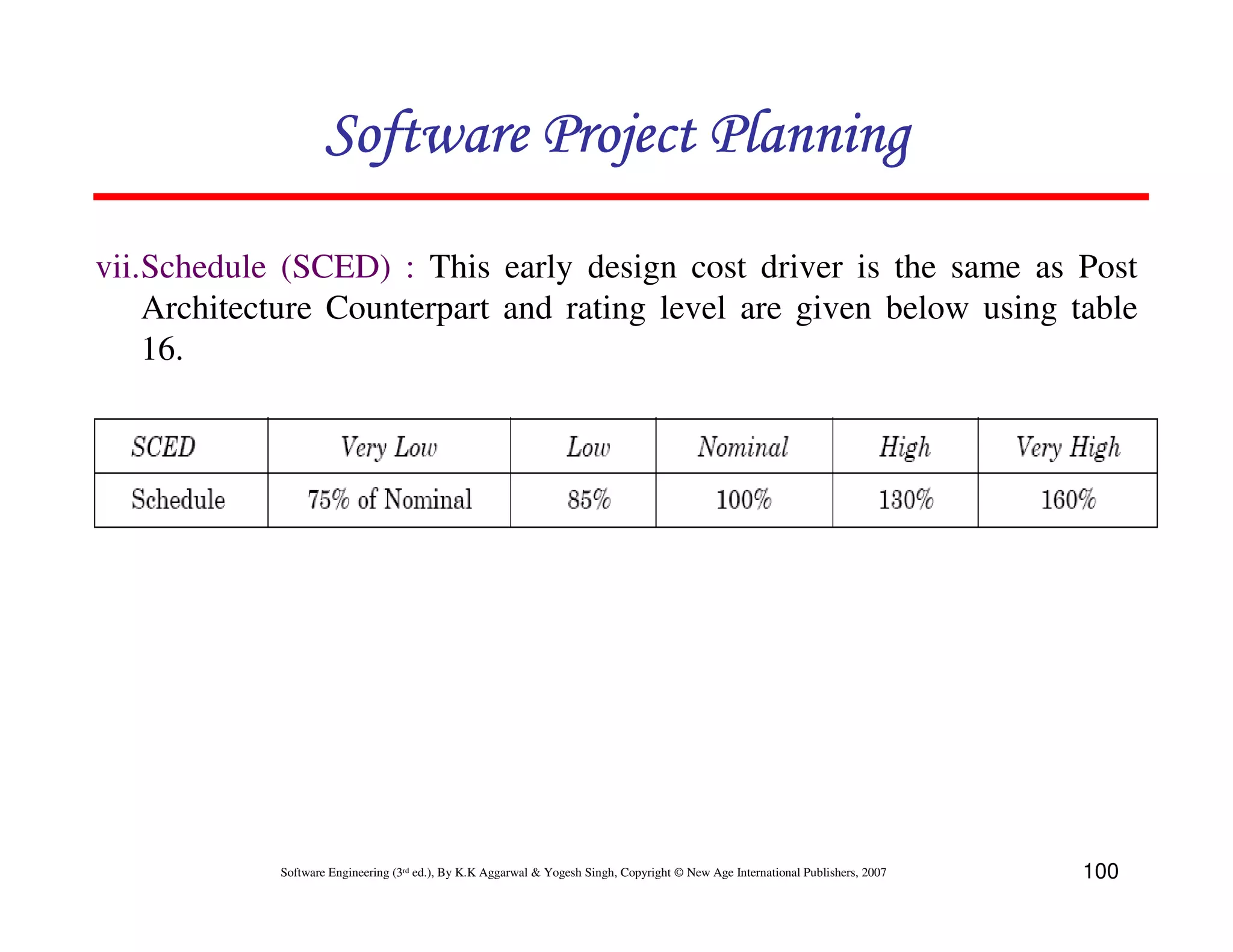
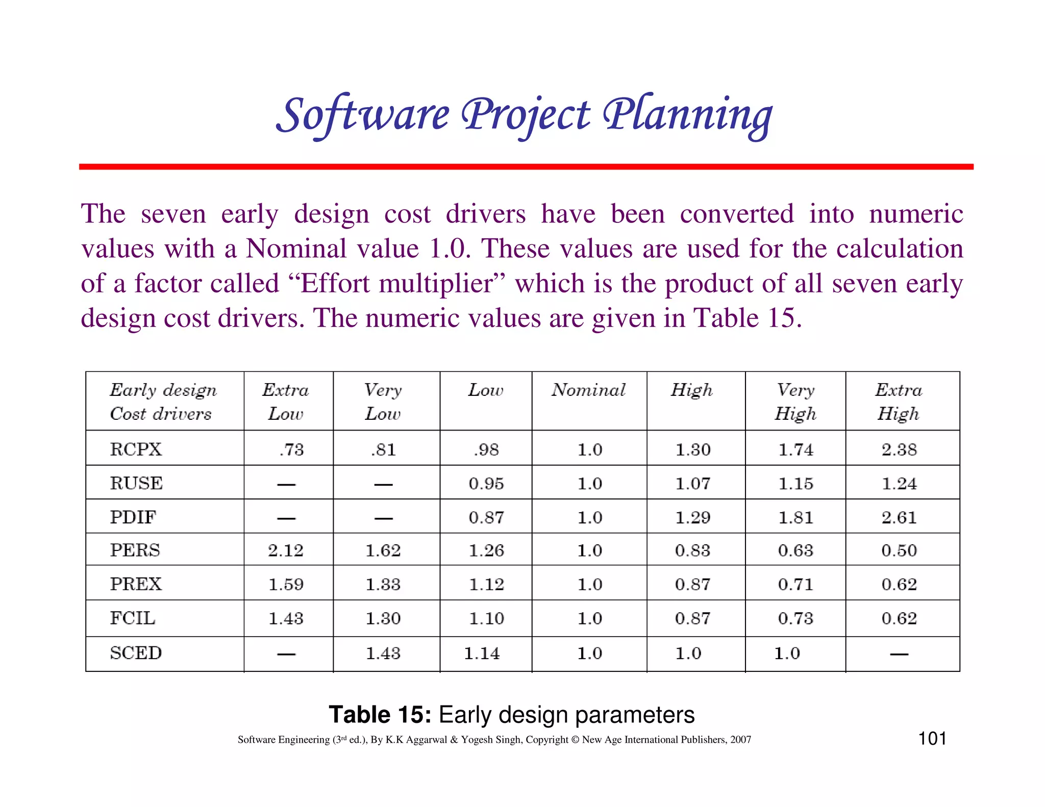
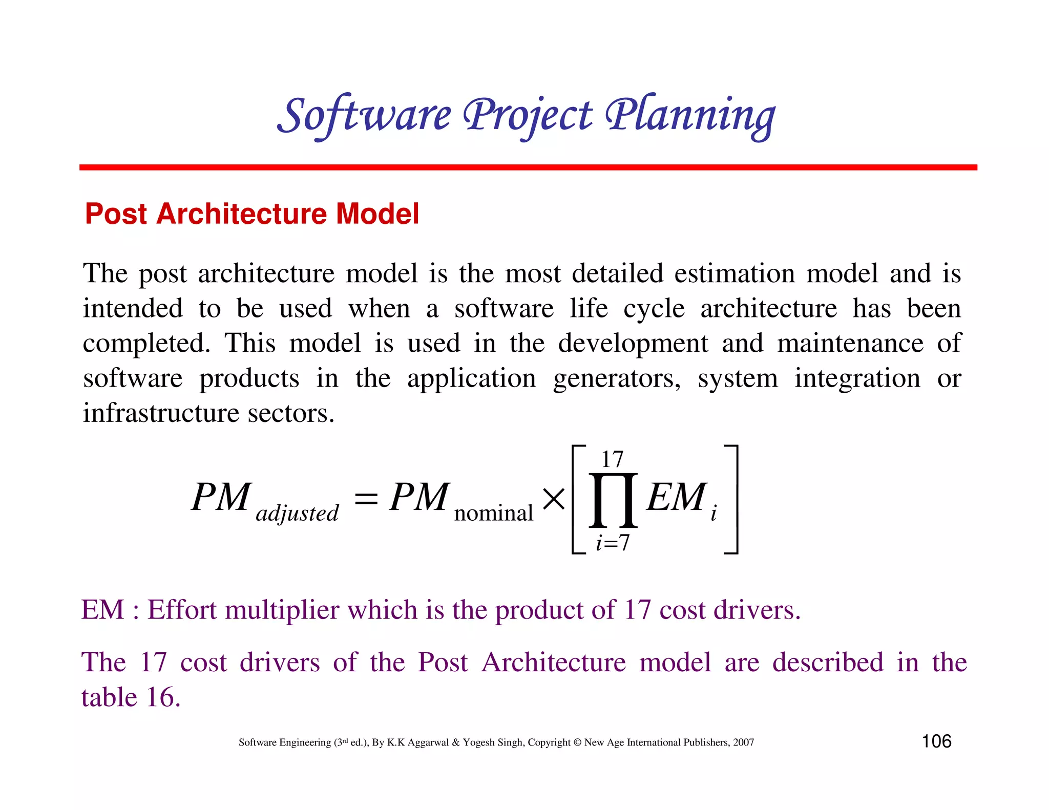
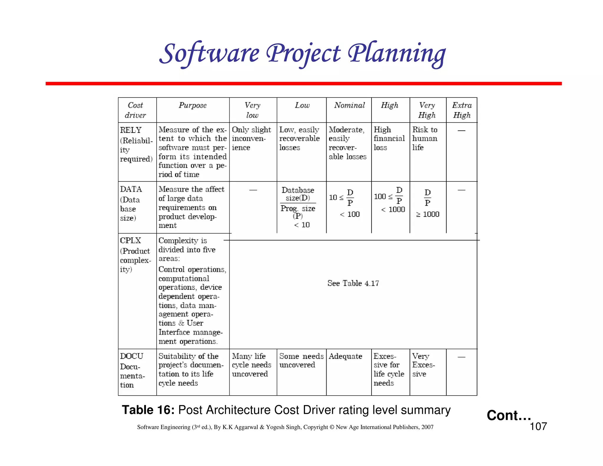
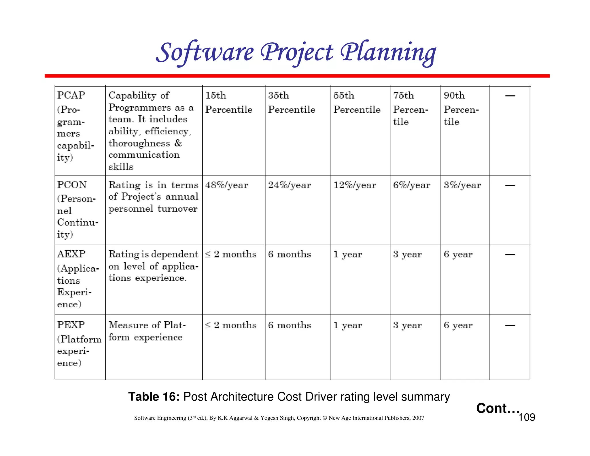
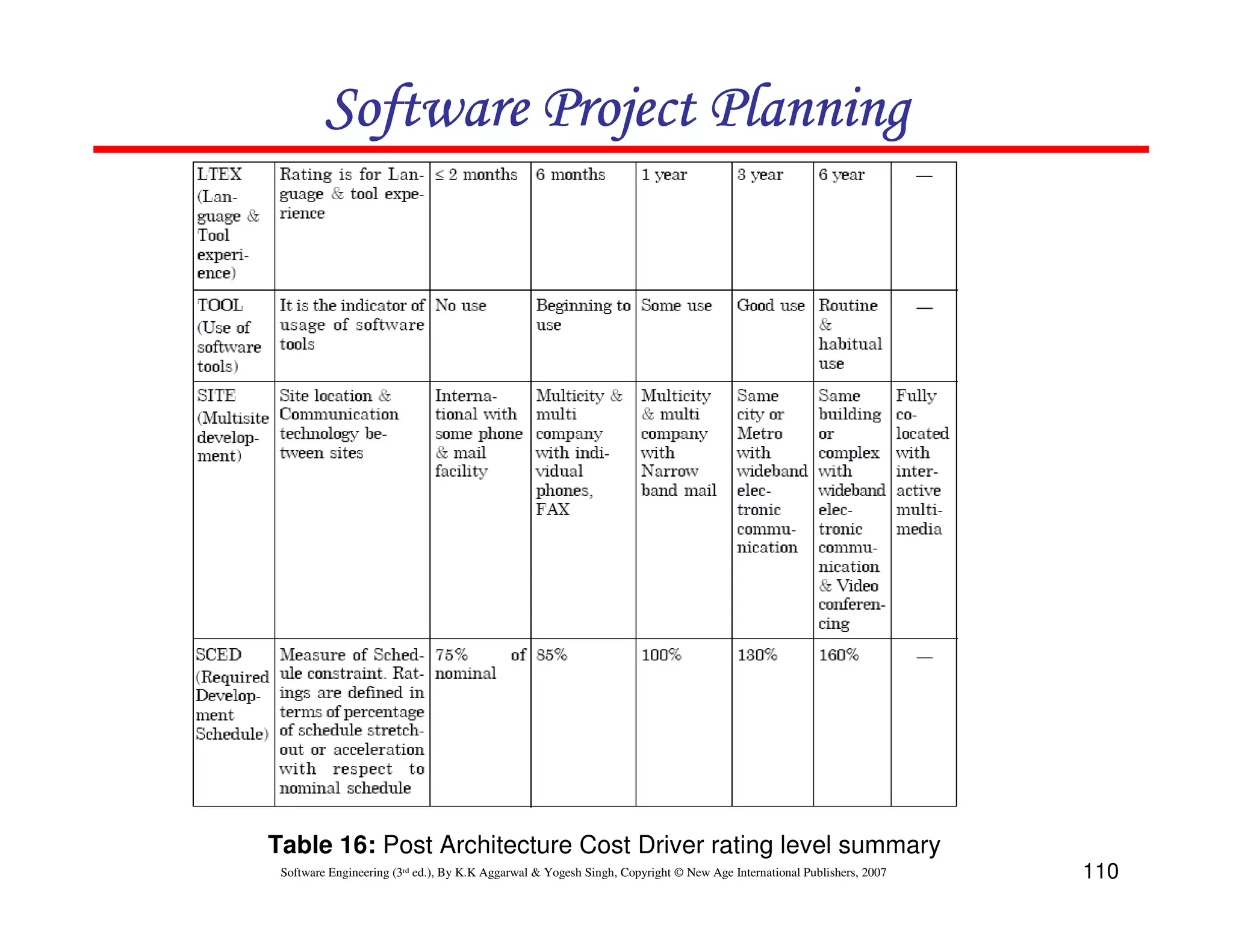
Cost drivers in early design and post-architecture models; Explains impact of product and personnel attributes on cost estimation.
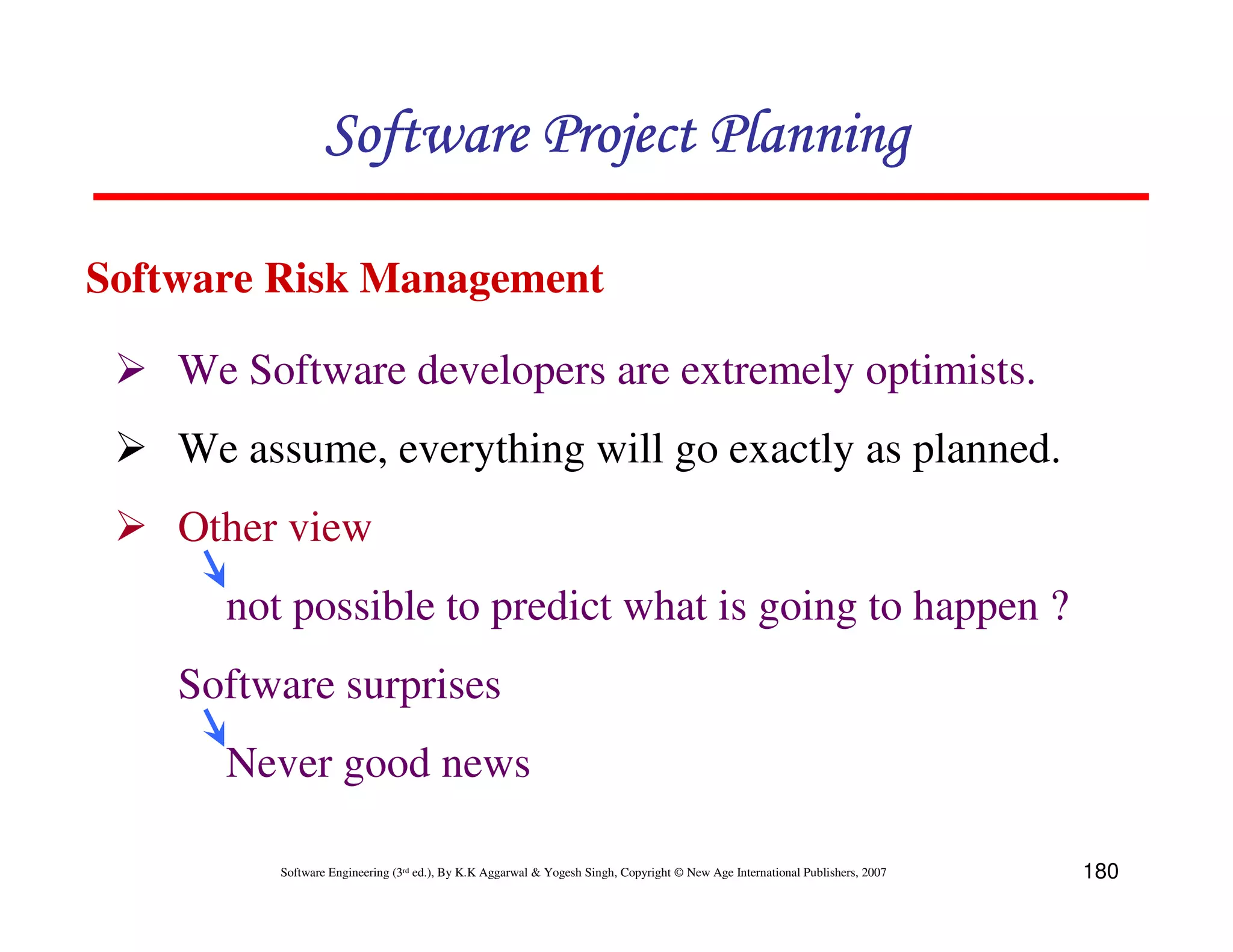
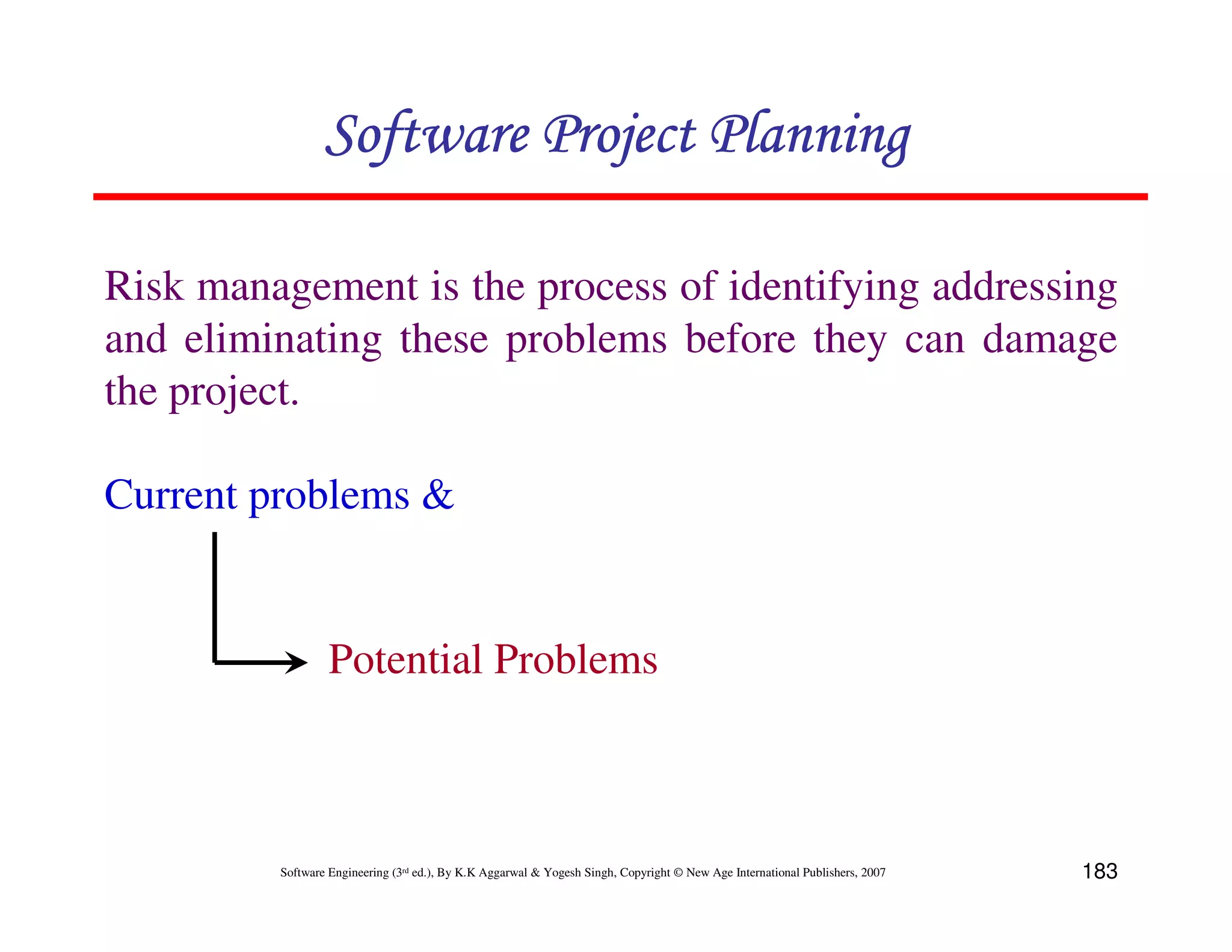
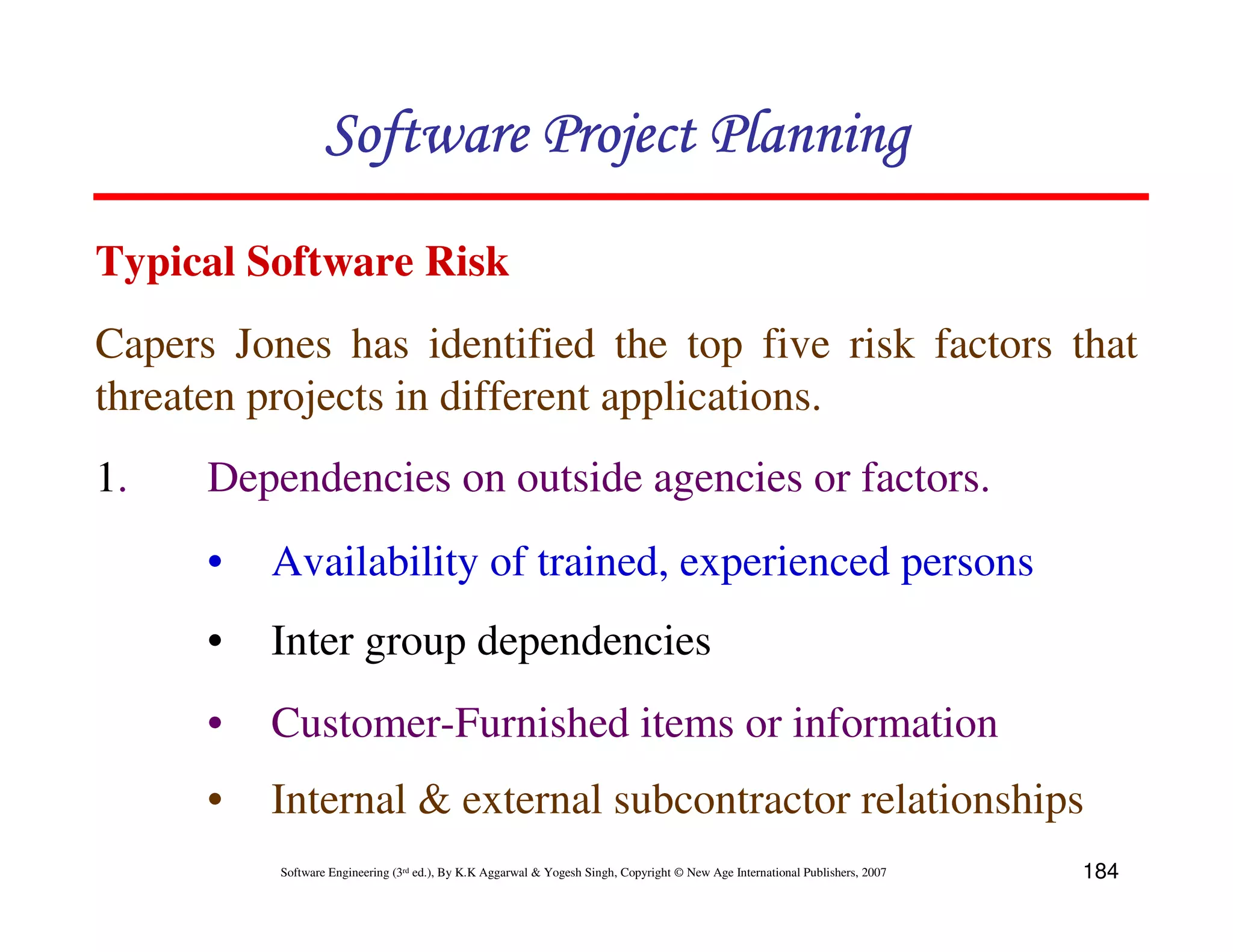
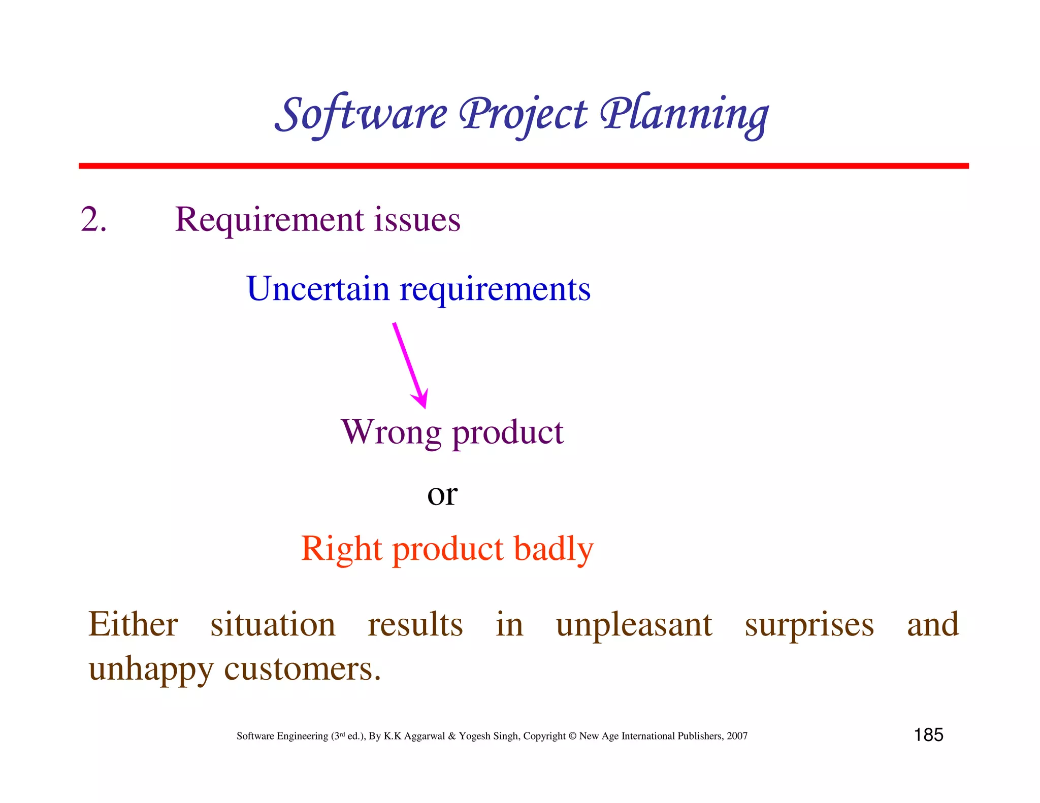
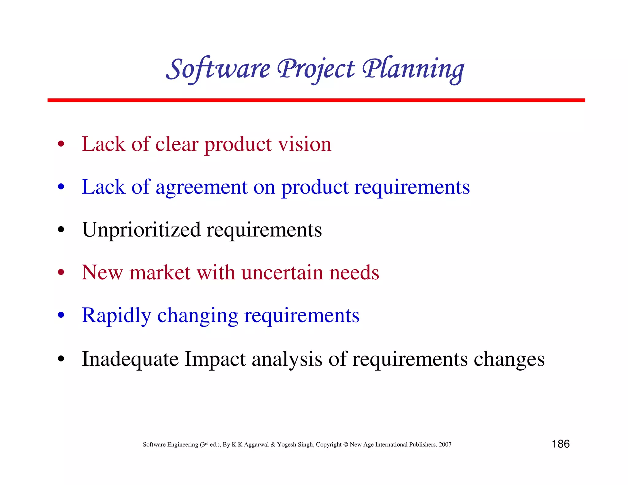
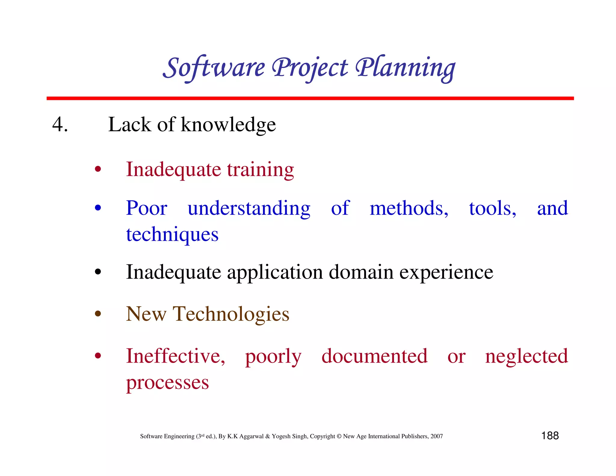
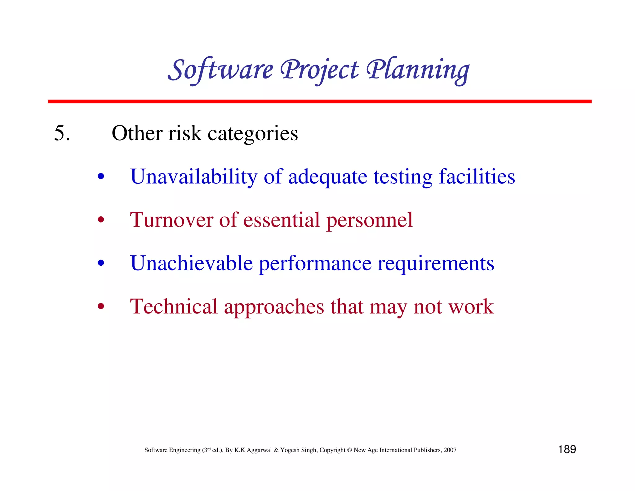
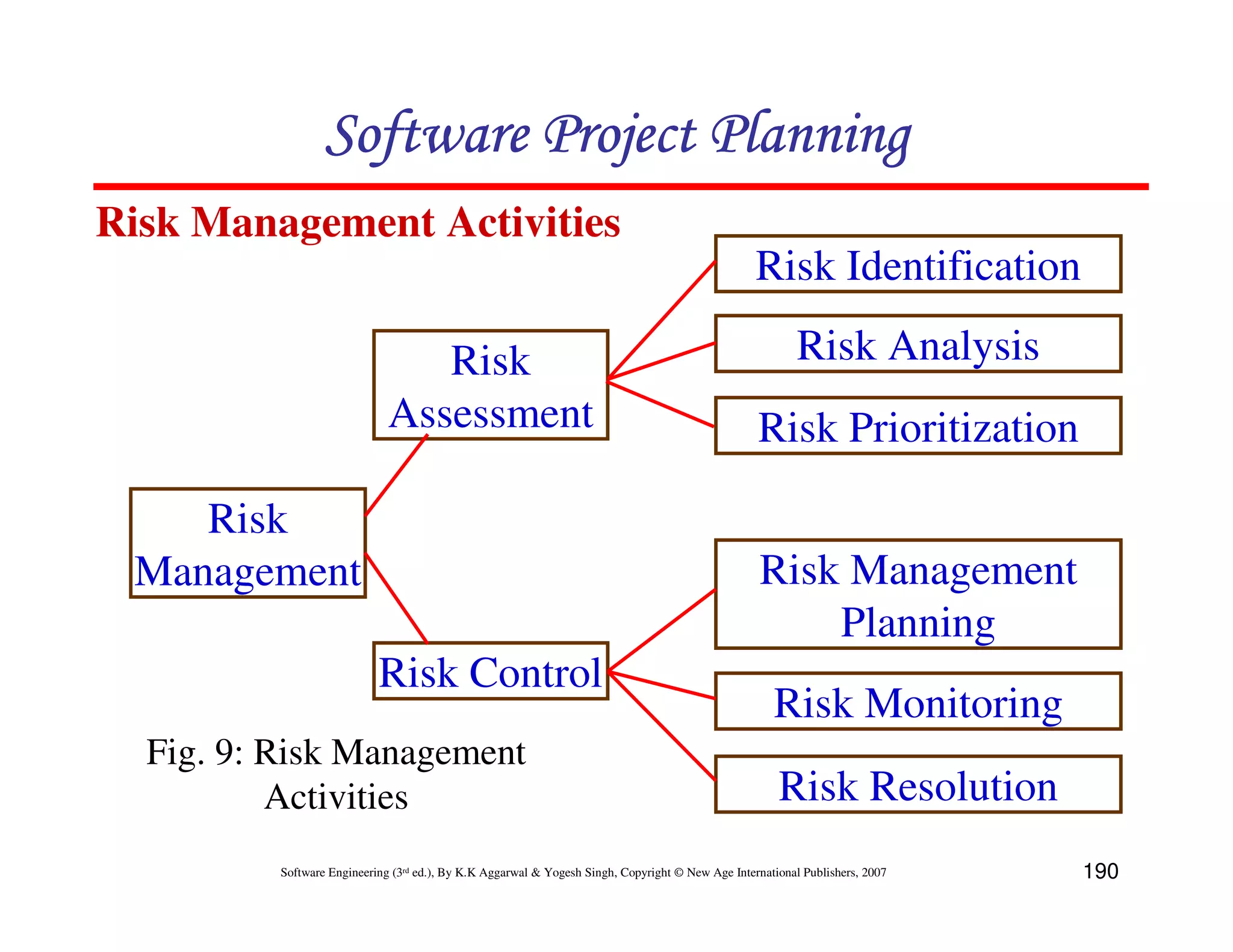
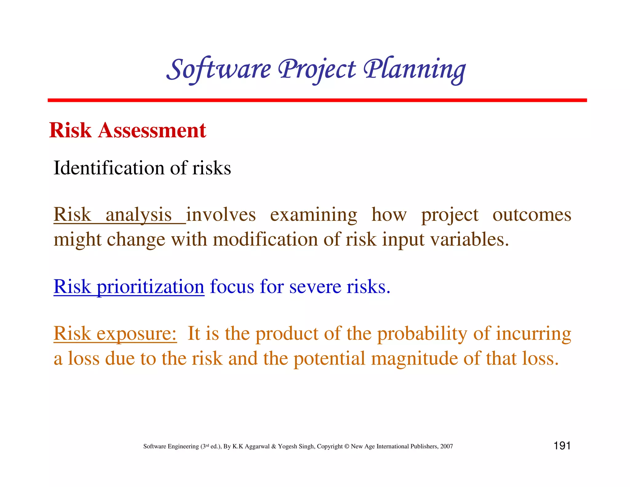
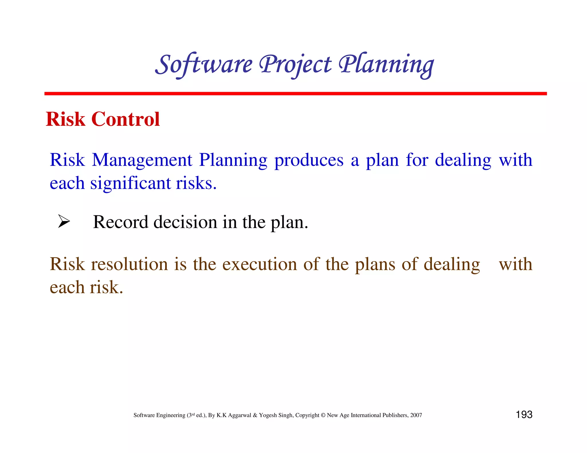
Identifies risks in software projects and emphasizes the importance of risk management activities to handle potential crises.
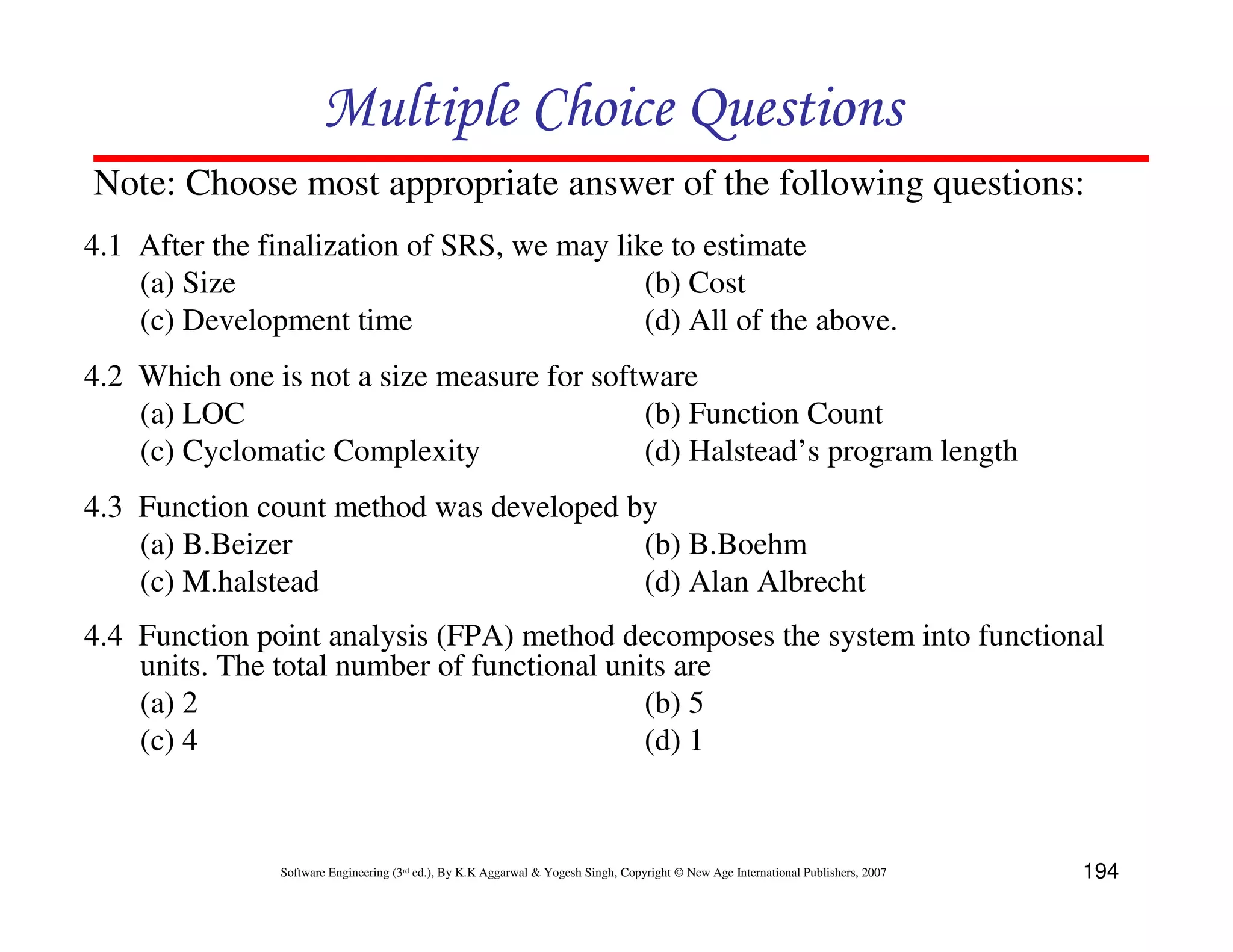
Includes various exercises for practical understanding of concepts like project planning, function points, COCOMO, and risk management.


![[slides] Software Engineering Third Edition - Aggarwal, Singh.pdf](https://cdn.slidesharecdn.com/ss_thumbnails/slidessoftwareengineeringthirdedition-aggarwalsingh-230615025923-02cadfc5-thumbnail.jpg?width=640&height=640&fit=bounds)