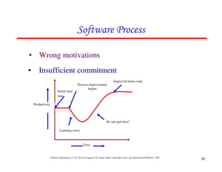
This document discusses common myths and misconceptions in software engineering. It presents 14 common myths that are frequently believed but are generally false, such as the ideas that more features means better software, software quality can only be assessed through testing, or that adding more developers will solve schedule delays. The document aims to dispel these myths by explaining why each one is a misconception regarding the realities of software development.


![5
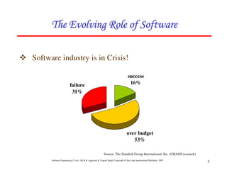
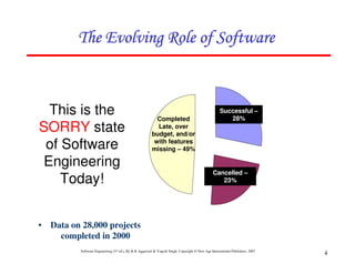
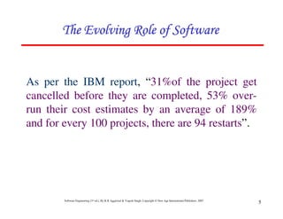
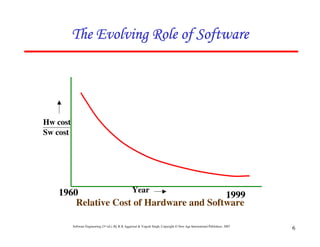
Software Engineering (3rd ed.), By K.K Aggarwal & Yogesh Singh, Copyright © New Age International Publishers, 2007
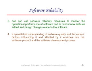
}
18.
return 0;
17.
}
16.
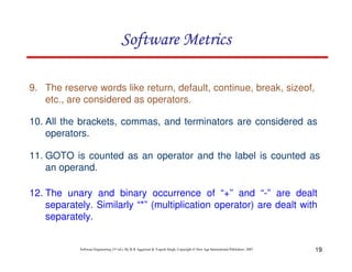
}
15.
x[j] = save;
14.
x[i] = x[j];
13.
Save = x[i];
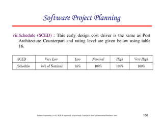
12.
{
11.
if (x[i] < x[j])
10.
for (j=1; j<=im; j++)
9.
im1=i-1;
8.
{
7.
for (i=2; i<=n; i++)
6.
If (n<2) return 1;
5.
/*This function sorts array x in ascending order */
4.
int i, j, save, im1;
3.
{
2.
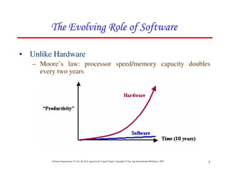
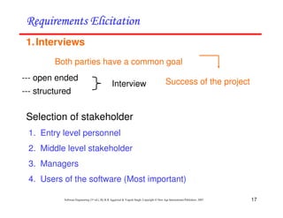
int. sort (int x[ ], int n)
1.
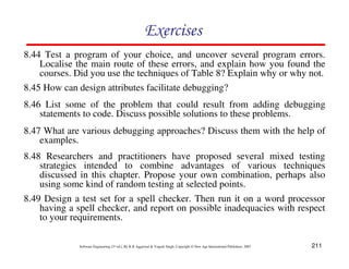
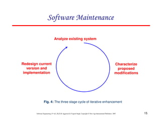
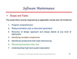
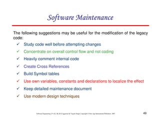
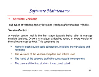
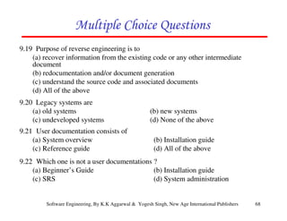
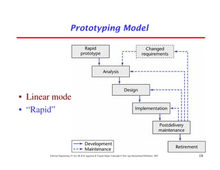
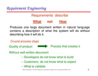
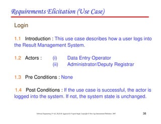
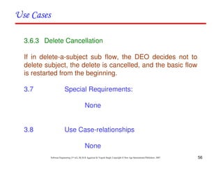
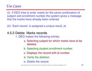
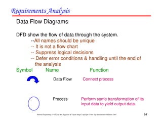
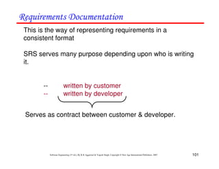
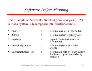
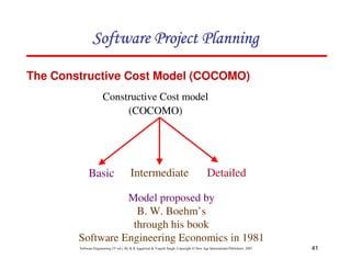
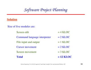
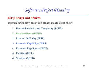
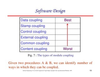
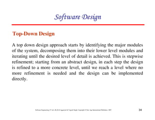
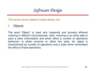
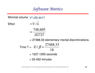
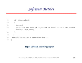
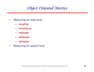
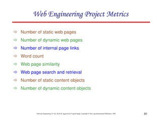
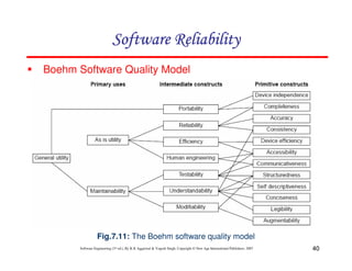
If LOC is simply a count of
the number of lines then
figure shown below contains
18 LOC .
When comments and blank
lines are ignored, the
program in figure 2 shown
below contains 17 LOC.
Lines of Code (LOC)
Size Estimation Fig. 2: Function for sorting an array](https://image.slidesharecdn.com/slidessoftwareengineeringthirdedition-aggarwalsingh-230615025923-02cadfc5/85/slides-Software-Engineering-Third-Edition-Aggarwal-Singh-pdf-274-320.jpg)


![20
Software Engineering (3rd ed.), By K.K Aggarwal & Yogesh Singh, Copyright © New Age International Publishers, 2007
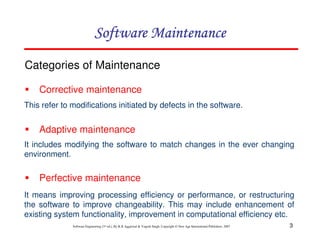
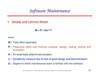
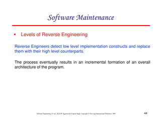
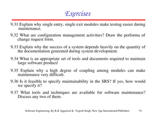
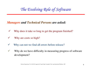
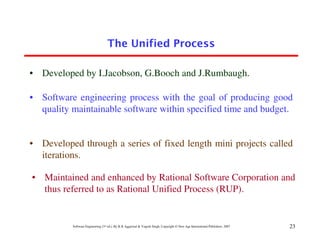
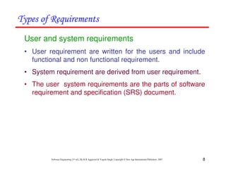
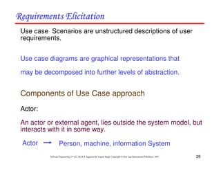
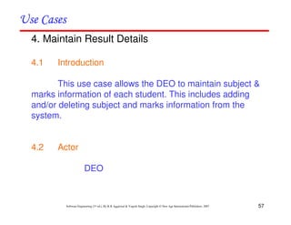
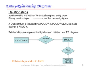
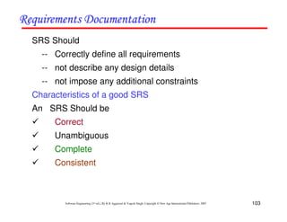
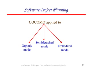
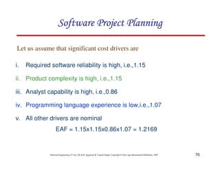
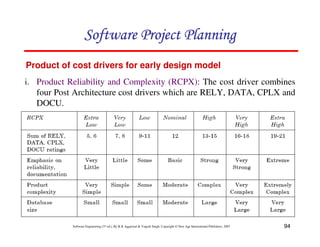
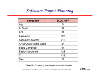
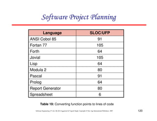
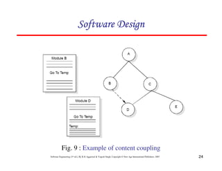
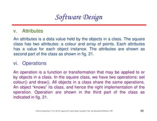
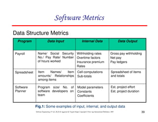
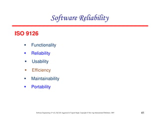
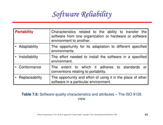
Organizations that use function point methods develop a criterion for
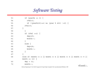
determining whether a particular entry is Low, Average or High.
Nonetheless, the determination of complexity is somewhat
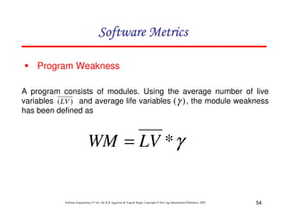
subjective.
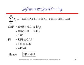
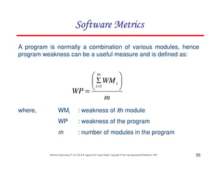
FP = UFP * CAF
Where CAF is complexity adjustment factor and is equal to [0.65 +
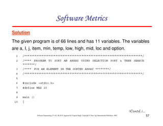
0.01 x Fi]. The Fi (i=1 to 14) are the degree of influence and are
based on responses to questions noted in table 3.](https://image.slidesharecdn.com/slidessoftwareengineeringthirdedition-aggarwalsingh-230615025923-02cadfc5/85/slides-Software-Engineering-Third-Edition-Aggarwal-Singh-pdf-289-320.jpg)


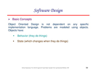
![117
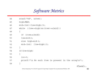
Software Engineering (3rd ed.), By K.K Aggarwal & Yogesh Singh, Copyright © New Age International Publishers, 2007
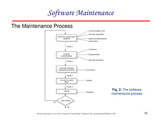
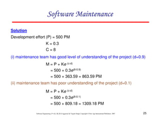
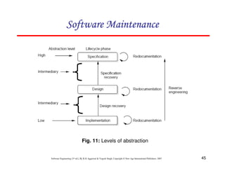
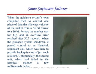
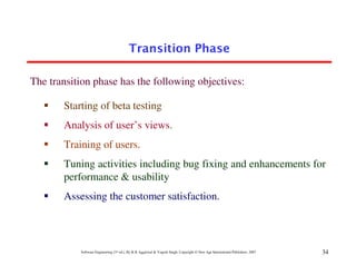
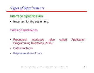
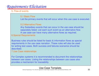
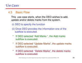
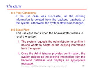
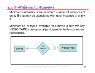
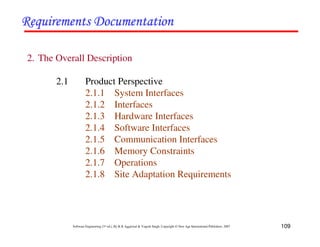
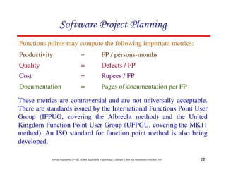
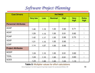
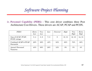
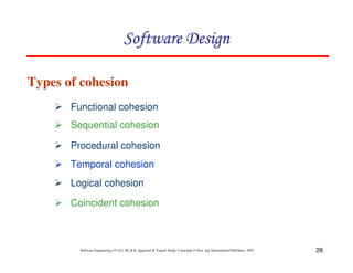
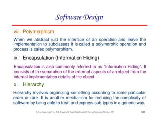
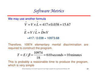
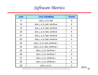
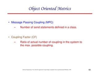
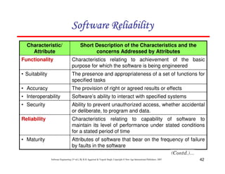
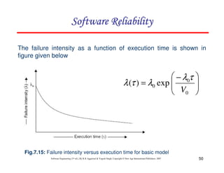
Schedule estimation
Development time can be calculated using PMadjusted as a key factor and the
desired equation is:
100
%
)
(
[ ))]
091
.
0
(
2
.
0
28
.
0
(
nominal
SCED
PM
TDEV B
adjusted ∗
×
= −
+
φ
where = constant, provisionally set to 3.67
TDEVnominal = calendar time in months with a scheduled constraint
B = Scaling factor
PMadjusted = Estimated effort in Person months (after adjustment)](https://image.slidesharecdn.com/slidessoftwareengineeringthirdedition-aggarwalsingh-230615025923-02cadfc5/85/slides-Software-Engineering-Third-Edition-Aggarwal-Singh-pdf-386-320.jpg)


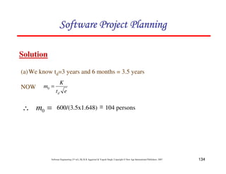
![125
Software Engineering (3rd ed.), By K.K Aggarwal & Yogesh Singh, Copyright © New Age International Publishers, 2007
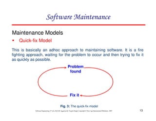
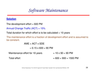
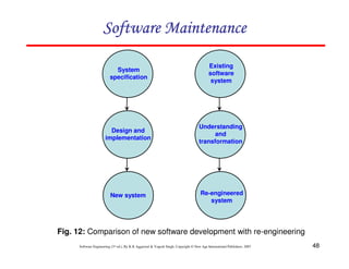
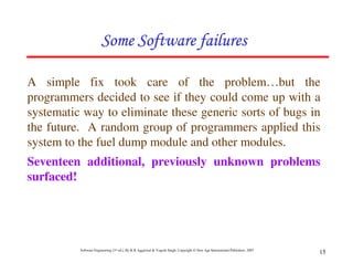
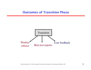
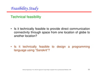
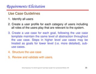
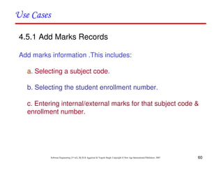
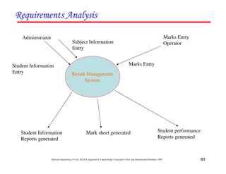
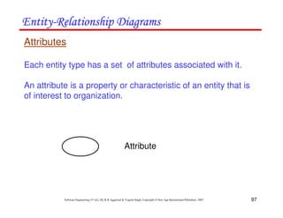
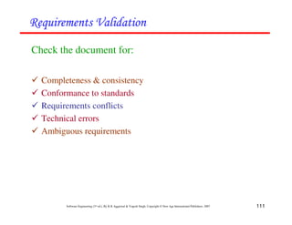
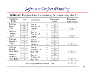
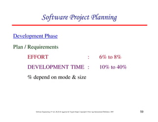
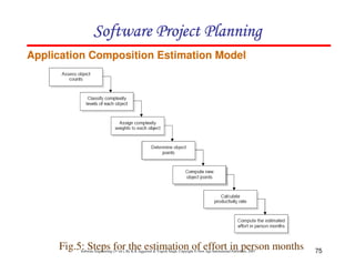
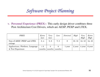
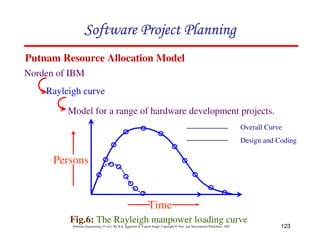
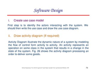
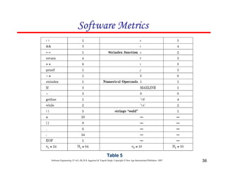
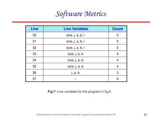
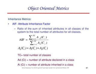
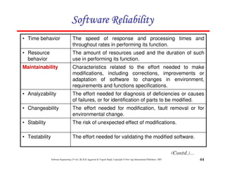
The Norden / Rayleigh Curve
= manpower utilization rate per unit time
a = parameter that affects the shape of the curve
K = area under curve in the interval [0, ]
t = elapsed time
dt
dy
2
2
)
( at
kate
dt
dy
t
m −
=
= --------- (1)
The curve is modeled by differential equation](https://image.slidesharecdn.com/slidessoftwareengineeringthirdedition-aggarwalsingh-230615025923-02cadfc5/85/slides-Software-Engineering-Third-Edition-Aggarwal-Singh-pdf-394-320.jpg)
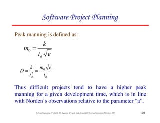
![126
Software Engineering (3rd ed.), By K.K Aggarwal & Yogesh Singh, Copyright © New Age International Publishers, 2007
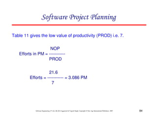
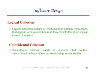
On Integration on interval [o, t]
Where y(t): cumulative manpower used upto time t.
y(0) = 0
y( ) = k
y(t) = K [1-e-at2
] -------------(2)
The cumulative manpower is null at the start of the project, and
grows monotonically towards the total effort K (area under the
curve).](https://image.slidesharecdn.com/slidessoftwareengineeringthirdedition-aggarwalsingh-230615025923-02cadfc5/85/slides-Software-Engineering-Third-Edition-Aggarwal-Singh-pdf-395-320.jpg)
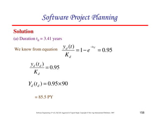
![127
Software Engineering (3rd ed.), By K.K Aggarwal & Yogesh Singh, Copyright © New Age International Publishers, 2007
0
]
2
1
[
2 2
2
2
2
=
−
= −
at
kae
dt
y
d at
a
td
2
1
2
=
“td”: time where maximum effort rate occurs
Replace “td” for t in equation (2)
2
5
.
0
2
2
1
3935
.
0
)
(
)
1
(
1
)
(
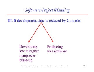
2
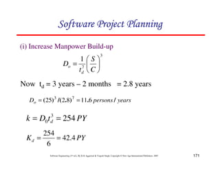
2
d
t
t
t
a
k
t
y
E
e
K
e
k
t
y
E d
d
=
=
=
−
=
−
=
= −](https://image.slidesharecdn.com/slidessoftwareengineeringthirdedition-aggarwalsingh-230615025923-02cadfc5/85/slides-Software-Engineering-Third-Edition-Aggarwal-Singh-pdf-396-320.jpg)


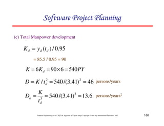
![135
Software Engineering (3rd ed.), By K.K Aggarwal & Yogesh Singh, Copyright © New Age International Publishers, 2007
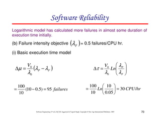
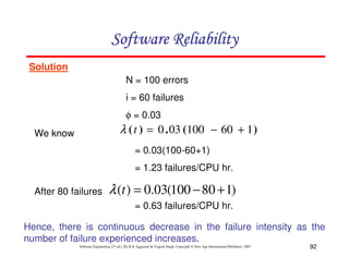
(b) We know
[ ]
2
1
)
( at
e
K
t
y −
−
=
t = 1 year and 2 months
= 1.17 years
041
.
0
)
5
.
3
(
2
1
2
1
2
2
=
×
=
=
d
t
a
[ ]
2
)
17
.
1
(
041
.
0
1
600
)
17
.
1
( −
−
= e
y
= 32.6 PY](https://image.slidesharecdn.com/slidessoftwareengineeringthirdedition-aggarwalsingh-230615025923-02cadfc5/85/slides-Software-Engineering-Third-Edition-Aggarwal-Singh-pdf-404-320.jpg)


![153
Software Engineering (3rd ed.), By K.K Aggarwal & Yogesh Singh, Copyright © New Age International Publishers, 2007
An examination of md(t) function shows a non-zero value of md
at time td.
This is because the manpower involved in design & coding is
still completing this activity after td in form of rework due to
the validation of the product.
Nevertheless, for the model, a level of completion has to be
assumed for development.
It is assumed that 95% of the development will be completed
by the time td.
md (t) = 2kdbt e-bt2
yd (t) = Kd [1-e-bt2
]
∴](https://image.slidesharecdn.com/slidessoftwareengineeringthirdedition-aggarwalsingh-230615025923-02cadfc5/85/slides-Software-Engineering-Third-Edition-Aggarwal-Singh-pdf-422-320.jpg)


![20
Software Engineering (3rd ed.), By K.K Aggarwal & Yogesh Singh, Copyright © New Age International Publishers, 2007
15. All the hash directive are ignored.
14. In the structure variables such as “struct-name, member-name”
or “struct-name -> member-name”, struct-name, member-name
are taken as operands and ‘.’, ‘->’ are taken as operators. Some
names of member elements in different structure variables are
counted as unique operands.
13. In the array variables such as “array-name [index]” “array-
name” and “index” are considered as operands and [ ] is
considered as operator.](https://image.slidesharecdn.com/slidessoftwareengineeringthirdedition-aggarwalsingh-230615025923-02cadfc5/85/slides-Software-Engineering-Third-Edition-Aggarwal-Singh-pdf-595-320.jpg)


![72
Software Engineering (3rd ed.), By K.K Aggarwal & Yogesh Singh, Copyright © New Age International Publishers, 2007
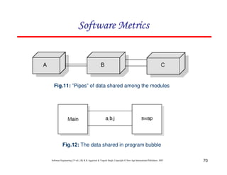
1. ‘FAN IN’ is simply a count of the number of other Components
that can call, or pass control, to Component A.
2. ‘FANOUT’ is the number of Components that are called by
Component A.
3. This is derived from the first two by using the following formula.
We will call this measure the INFORMATION FLOW index of
Component A, abbreviated as IF(A).
The Basic Information Flow Model
Information Flow metrics are applied to the Components of a
system design. Fig. 13 shows a fragment of such a design, and for
component ‘A’ we can define three measures, but remember that
these are the simplest models of IF.
IF(A) = [FAN IN(A) x FAN OUT (A)]2](https://image.slidesharecdn.com/slidessoftwareengineeringthirdedition-aggarwalsingh-230615025923-02cadfc5/85/slides-Software-Engineering-Third-Edition-Aggarwal-Singh-pdf-647-320.jpg)


![15
Software Engineering (3rd ed.), By K.K Aggarwal & Yogesh Singh, Copyright © New Age International Publishers, 2007
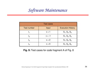
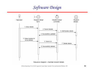
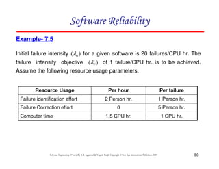
Fig. 5: Input domain of two variables x and y with
boundaries [100,300] each
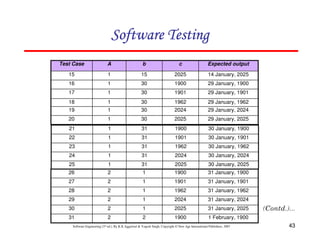
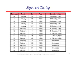
The boundary value analysis test cases for our program with two inputs
variables (x and y) that may have any value from 100 to 300 are: (200,100),
(200,101), (200,200), (200,299), (200,300), (100,200), (101,200), (299,200) and
(300,200). This input domain is shown in Fig. 8.5. Each dot represent a test case
and inner rectangle is the domain of legitimate inputs. Thus, for a program of n
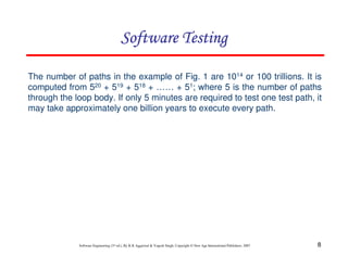
variables, boundary value analysis yield 4n + 1 test cases.
y
x
Input domain
300
200
100
400
0 300
200
100 400](https://image.slidesharecdn.com/slidessoftwareengineeringthirdedition-aggarwalsingh-230615025923-02cadfc5/85/slides-Software-Engineering-Third-Edition-Aggarwal-Singh-pdf-822-320.jpg)
![16
Software Engineering (3rd ed.), By K.K Aggarwal & Yogesh Singh, Copyright © New Age International Publishers, 2007
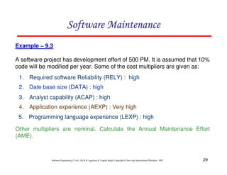
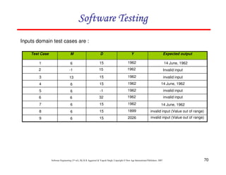
Example- 8.I
Consider a program for the determination of the nature of roots of a
quadratic equation. Its input is a triple of positive integers (say a,b,c) and
values may be from interval [0,100]. The program output may have one of
the following words.
[Not a quadratic equation; Real roots; Imaginary roots; Equal roots]
Design the boundary value test cases.](https://image.slidesharecdn.com/slidessoftwareengineeringthirdedition-aggarwalsingh-230615025923-02cadfc5/85/slides-Software-Engineering-Third-Edition-Aggarwal-Singh-pdf-823-320.jpg)


![22
Software Engineering (3rd ed.), By K.K Aggarwal & Yogesh Singh, Copyright © New Age International Publishers, 2007
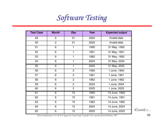
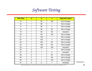
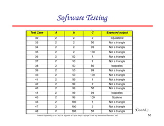
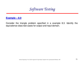
Example – 8.3
Consider a simple program to classify a triangle. Its inputs is a triple of
positive integers (say x, y, z) and the date type for input parameters ensures
that these will be integers greater than 0 and less than or equal to 100. The
program output may be one of the following words:
[Scalene; Isosceles; Equilateral; Not a triangle]
Design the boundary value test cases.](https://image.slidesharecdn.com/slidessoftwareengineeringthirdedition-aggarwalsingh-230615025923-02cadfc5/85/slides-Software-Engineering-Third-Edition-Aggarwal-Singh-pdf-829-320.jpg)


![25
Software Engineering (3rd ed.), By K.K Aggarwal & Yogesh Singh, Copyright © New Age International Publishers, 2007
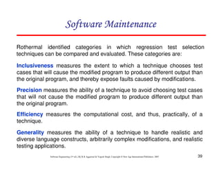
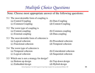
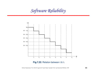
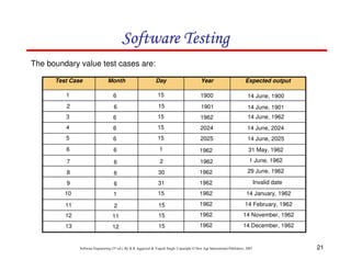
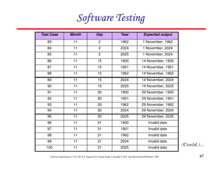
Fig. 8.6: Robustness test cases for two variables x
and y with range [100,300] each
y
x
300
200
100
400
0 300
200
100 400](https://image.slidesharecdn.com/slidessoftwareengineeringthirdedition-aggarwalsingh-230615025923-02cadfc5/85/slides-Software-Engineering-Third-Edition-Aggarwal-Singh-pdf-832-320.jpg)


![61
Software Engineering (3rd ed.), By K.K Aggarwal & Yogesh Singh, Copyright © New Age International Publishers, 2007
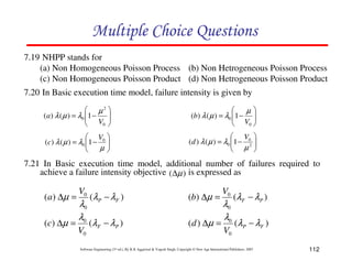
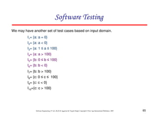
In this method, input domain of a program is partitioned into a finite number of
equivalence classes such that one can reasonably assume, but not be
absolutely sure, that the test of a representative value of each class is
equivalent to a test of any other value.
Two steps are required to implementing this method:
Equivalence Class Testing
1. The equivalence classes are identified by taking each input condition and
partitioning it into valid and invalid classes. For example, if an input
condition specifies a range of values from 1 to 999, we identify one valid
equivalence class [1<item<999]; and two invalid equivalence classes
[item<1] and [item>999].
2. Generate the test cases using the equivalence classes identified in the
previous step. This is performed by writing test cases covering all the valid
equivalence classes. Then a test case is written for each invalid equivalence
class so that no test contains more than one invalid class. This is to ensure
that no two invalid classes mask each other.](https://image.slidesharecdn.com/slidessoftwareengineeringthirdedition-aggarwalsingh-230615025923-02cadfc5/85/slides-Software-Engineering-Third-Edition-Aggarwal-Singh-pdf-868-320.jpg)


![118
Software Engineering (3rd ed.), By K.K Aggarwal & Yogesh Singh, Copyright © New Age International Publishers, 2007
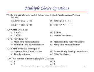
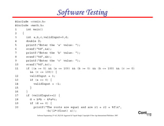
Example 8.13
Consider the problem for the determination of the nature of roots of a quadratic
equation. Its input a triple of positive integers (say a,b,c) and value may be from
interval [0,100].
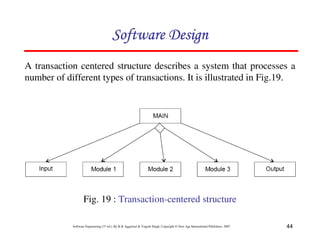
The program is given in fig. 19. The output may have one of the following words:
[Not a quadratic equation; real roots; Imaginary roots; Equal roots]
Draw the flow graph and DD path graph. Also find independent paths from the DD
Path graph.](https://image.slidesharecdn.com/slidessoftwareengineeringthirdedition-aggarwalsingh-230615025923-02cadfc5/85/slides-Software-Engineering-Third-Edition-Aggarwal-Singh-pdf-925-320.jpg)


![125
Software Engineering (3rd ed.), By K.K Aggarwal & Yogesh Singh, Copyright © New Age International Publishers, 2007
Example 8.14
Consider a program given in Fig.8.20 for the classification of a triangle. Its input is a
triple of positive integers (say a,b,c) from the interval [1,100]. The output may be
[Scalene, Isosceles, Equilateral, Not a triangle].
Draw the flow graph & DD Path graph. Also find the independent paths from the DD
Path graph.](https://image.slidesharecdn.com/slidessoftwareengineeringthirdedition-aggarwalsingh-230615025923-02cadfc5/85/slides-Software-Engineering-Third-Edition-Aggarwal-Singh-pdf-932-320.jpg)


![153
Software Engineering (3rd ed.), By K.K Aggarwal & Yogesh Singh, Copyright © New Age International Publishers, 2007
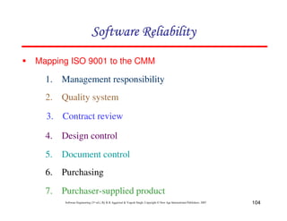
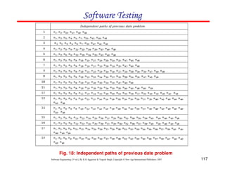
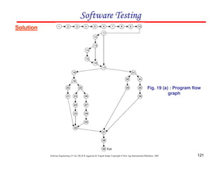
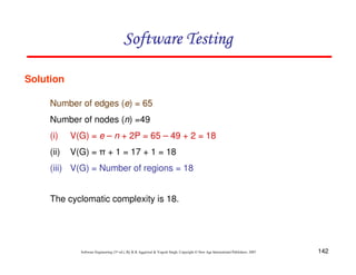
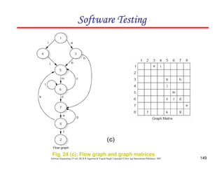
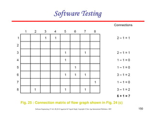
Solution
The graph & connection matrices are given below :
To find two link paths, we have to generate a square of graph matrix [A] and for three
link paths, a cube of matrix [A] is required.](https://image.slidesharecdn.com/slidessoftwareengineeringthirdedition-aggarwalsingh-230615025923-02cadfc5/85/slides-Software-Engineering-Third-Edition-Aggarwal-Singh-pdf-960-320.jpg)


![159
Software Engineering (3rd ed.), By K.K Aggarwal & Yogesh Singh, Copyright © New Age International Publishers, 2007
Example 8.20
Consider the program of the determination of the nature of roots of a quadratic
equation. Its input is a triple of positive integers (say a,b,c) and values for each of
these may be from interval [0,100]. The program is given in Fig. 19. The output may
have one of the option given below:
(i) Not a quadratic program
(ii) real roots
(iii) imaginary roots
(iv) equal roots
(v) invalid inputs
Find all du-paths and identify those du-paths that are definition clear.](https://image.slidesharecdn.com/slidessoftwareengineeringthirdedition-aggarwalsingh-230615025923-02cadfc5/85/slides-Software-Engineering-Third-Edition-Aggarwal-Singh-pdf-966-320.jpg)


![163
Software Engineering (3rd ed.), By K.K Aggarwal & Yogesh Singh, Copyright © New Age International Publishers, 2007
Example 8.21
Consider the program given in Fig. 20 for the classification of a triangle. Its
input is a triple of positive integers (say a,b,c) from the interval [1,100]. The
output may be:
[Scalene, Isosceles, Equilateral, Not a triangle, Invalid inputs].
Find all du-paths and identify those du-paths that are definition clear.](https://image.slidesharecdn.com/slidessoftwareengineeringthirdedition-aggarwalsingh-230615025923-02cadfc5/85/slides-Software-Engineering-Third-Edition-Aggarwal-Singh-pdf-970-320.jpg)