Q#1AgePopulationUnder 5 years19,853,515Question:Breakdown Population of U.S with respect to age?5 to 9 years20,445,12210 to 14 years20,713,11115 to 19 years21,219,05020 to 24 years22,501,96525 to 34 years44,044,17335 to 44 years40,656,41945 to 54 years43,091,14355 to 59 years21,523,46060 to 64 years19,224,06065 to 74 years27,503,38975 to 84 years14,087,47785 years and over6,141,523
Scatter plot
Under 5 years 5 to 9 years 10 to 14 years 15 to 19 years 20 to 24 years 25 to 34 years 35 to 44 years 45 to 54 years 55 to 59 years 60 to 64 years 65 to 74 years 75 to 84 years 85 years and over 19853515 20445122 20713111 21219050 22501965 44044173 40656419 43091143 21523460 19224060 27503389 14087477 6141523
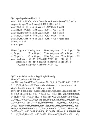
Q#2Sales Price of Existing Single-Family HomesYearMonthU.SNorth eastMidwestSouthWestQuestion:20164,838,000617,0001,222,0001,955,0001,044,000What is the difference in sale amount of single family homes in different parts of US?20174,892,000615,0001,222,0001,989,0001,066,00020184,742,000581,0001,192,0001,972,000997,0002018Jul4,790,000580,0001,190,0001,980,0001,040,0002018Aug4,760,000590,0001,210,0001,970,000990,0002018Sep4,600,000570,0001,190,0001,890,000950,0002018Oct4,620,000580,0001,180,0001,910,000950,0002018Nov4,630,000600,0001,220,0001,900,000910,0002018Dec4,450,000570,0001,120,0001,850,000910,0002019Jan4,360,000570,0001,090,0001,820,000880,0002019Feb4,910,000580,0001,190,0002,110,0001,030,0002019Mar4,670,000570,0001,100,0002,040,000960,0002019Apr4,630,000540,0001,110,0002,000,000980,0002019May4,760,000570,0001,160,0002,040,000990,0002019Jun4,710,000570,0001,180,0002,000,000960,0002019Jul4,840,000570,0001,200,0002,030,0001,040,000
Clustred column chart of Sale amoount in 1000s of Single family Homes
U.S Jul Aug Sep Oct Nov 2016 2017 2018 2018 2018 2018 2018 2018 4838000 4892000 4742000 4790000 4760000 4600000 4620000 4630000 North east Jul Aug Sep Oct Nov 2016 2017 2018 2018 2018 2018 2018 2018 617000 615000 581000 580000 590000 570000 580000 600000 Midwest Jul Aug Sep Oct Nov 2016 2017 2018 2018 2018 2018 2018 2018 1222000 1222000 1192000 1190000 1210000 1190000 1180000 1220000 South Jul Aug Sep Oct Nov 2016 2017 2018 2018 2018 2018 2018 2018 1955000 1989000 1972000 1980000 1970000 1890000 1910000 1900000 West Jul Aug Sep Oct Nov 2016 2017 2018 2018 2018 2018 2018 2018 1044000 1066000 997000 1040000 990000 950000 950000 910000
Q#3Provisional number of marriages and marriage rate: United States, 2000-2017YearMarriagesPopulationRate per 1,000 total populationQuestion:How number of marriages varries in U.S from 2000 to 2017?20172,236,496325,719,1786.920162,251,411323,127,5137.020152,221,579321,418,8206.92014 12,140,272308,759,7136.92013 12,081,301306,136,6726.820122,131,000313,914,0406.820112,118,000311,591,9176.820102,096,000308,745,5386.820092,080,000306,771,5296.820082,157,000304,093,9667.120072,197,000301,231,2077.32006 22,193,000294,077,2477.520052,249,000295,516,5997.620042,279,000292,805,2987.820032,245,000290,107,9337.720022, ...
1. Q#1AgePopulationUnder 5
years19,853,515Question:Breakdown Population of U.S with
respect to age?5 to 9 years20,445,12210 to 14
years20,713,11115 to 19 years21,219,05020 to 24
years22,501,96525 to 34 years44,044,17335 to 44
years40,656,41945 to 54 years43,091,14355 to 59
years21,523,46060 to 64 years19,224,06065 to 74
years27,503,38975 to 84 years14,087,47785 years and
over6,141,523
Scatter plot
Under 5 years 5 to 9 years 10 to 14 years 15 to 19 years 20
to 24 years 25 to 34 years 35 to 44 years 45 to 54 years 55
to 59 years 60 to 64 years 65 to 74 years 75 to 84 years 85
years and over 19853515 20445122 20713111 21219050
22501965 44044173 40656419 43091143 21523460
19224060 27503389 14087477 6141523
Q#2Sales Price of Existing Single-Family
HomesYearMonthU.SNorth
eastMidwestSouthWestQuestion:20164,838,000617,0001,222,00
01,955,0001,044,000What is the difference in sale amount of
single family homes in different parts of
US?20174,892,000615,0001,222,0001,989,0001,066,00020184,7
42,000581,0001,192,0001,972,000997,0002018Jul4,790,000580,
0001,190,0001,980,0001,040,0002018Aug4,760,000590,0001,21
0,0001,970,000990,0002018Sep4,600,000570,0001,190,0001,89
0,000950,0002018Oct4,620,000580,0001,180,0001,910,000950,
0002018Nov4,630,000600,0001,220,0001,900,000910,0002018
Dec4,450,000570,0001,120,0001,850,000910,0002019Jan4,360,
000570,0001,090,0001,820,000880,0002019Feb4,910,000580,00
01,190,0002,110,0001,030,0002019Mar4,670,000570,0001,100,
2. 0002,040,000960,0002019Apr4,630,000540,0001,110,0002,000,
000980,0002019May4,760,000570,0001,160,0002,040,000990,0
002019Jun4,710,000570,0001,180,0002,000,000960,0002019Jul
4,840,000570,0001,200,0002,030,0001,040,000
Clustred column chart of Sale amoount in 1000s of Single
family Homes
U.S Jul Aug Sep Oct Nov 2016 2017 2018 2018 2018 2018
2018 2018 4838000 4892000 4742000 4790000
4760000 4600000 4620000 4630000 North east
Jul Aug Sep Oct Nov 2016 2017 2018 2018 2018 2018
2018 2018 617000 615000 581000 580000 590000
570000 580000 600000 Midwest Jul Aug Sep
Oct Nov 2016 2017 2018 2018 2018 2018 2018 2018
1222000 1222000 1192000 1190000 1210000
1190000 1180000 1220000 South Jul Aug Sep
Oct Nov 2016 2017 2018 2018 2018 2018 2018 2018
1955000 1989000 1972000 1980000 1970000
1890000 1910000 1900000 West Jul Aug Sep Oct
Nov 2016 2017 2018 2018 2018 2018 2018 2018 1044000
1066000 997000 1040000 990000 950000 950000
910000
Q#3Provisional number of marriages and marriage rate: United
States, 2000-2017YearMarriagesPopulationRate per 1,000 total
populationQuestion:How number of marriages varries in U.S
from 2000 to
2017?20172,236,496325,719,1786.920162,251,411323,127,5137
.020152,221,579321,418,8206.92014
12,140,272308,759,7136.92013
12,081,301306,136,6726.820122,131,000313,914,0406.820112,
118,000311,591,9176.820102,096,000308,745,5386.820092,080
5. Q#2: What is the difference in sale amount of single-family
homes in different parts of US?
https://www.nar.realtor/sites/default/files/documents/ehs-07-
2019-single-family-only-2019-08-21.pdf
Units: (1000)
Clustred column chart of Sale amoount in 1000s of Single
family Homes
U.S Jul Aug Sep Oct Nov 2016 2017 2018 2018 2018 2018
2018 2018 4838000 4892000 4742000 4790000
4760000 4600000 4620000 4630000 North east
Jul Aug Sep Oct Nov 2016 2017 2018 2018 2018 2018
2018 2018 617000 615000 581000 580000 590000
570000 580000 600000 Midwest Jul Aug Sep
Oct Nov 2016 2017 2018 2018 2018 2018 2018 2018
1222000 1222000 1192000 1190000 1210000
1190000 1180000 1220000 South Jul Aug Sep
Oct Nov 2016 2017 2018 2018 2018 2018 2018 2018
1955000 1989000 1972000 1980000 1970000
1890000 1910000 1900000 West Jul Aug Sep Oct
Nov 2016 2017 2018 2018 2018 2018 2018 2018 1044000
1066000 997000 1040000 990000 950000 950000
910000
Q#3: How number of marriages varies in U.S from 2000 to
2017?
https://www.cdc.gov/nchs/data/dvs/national-marriage-divorce-
6. rates-00-17.pdf
Units(1000 person)
Marriages
2017 2016 2015 2014 1 2013 1 2012 2011 2010 2009 2008
2007 2006 2 2005 2004 2003 2002 2001 2000 2236496
2251411 2221579 2140272 2081301 2131000
2118000 2096000 2080000 2157000 2197000
2193000 2249000 2279000 2245000 2290000
2326000 2315000
Q#4: What is racial composition in U.S?
https://factfinder.census.gov/faces/tableservices/jsf/pages/produ
ctview.xhtml?pid=ACS_17_5YR_DP05&src=pt
[百分比]
White Black or African American American Indian
Asian Native Hawaiian Some other race 24297
2820 44631272 5487131 20371856 1327014 17282368
Q#5: What is the range of median Household income in U.S?
https://www.census.gov/data/academy/courses/excel.html
7. Frequency 45000 50000 55000 60000 65000
70000 More 5 13 9 4 4 3 5
Upper limit
Frequency
Data Analysis Project 1
For this project each student will learn and demonstrate
competency in researching economics; that is, creatively
designing a research question, locating pertinent and credible
data to support an answer, and presenting results in a
professional and articulate manner. The skill set practiced in
this project is highly valued in business and government
occupations. Follow these steps to complete the project:
1. Using the data covered in the Demography and Housing
slides, generate five research questions to study (e.g. “Have
home prices in the U.S. increased since 2010?”, “What is the
racial composition of U.S. males?”). You are to create two
research questions from Demography, two from Housing, and
one from either category. You are to use at least 3 different data
sources (e.g. census, CDC, NAR, etc.) in the overall project.
2. Excel File: For each research question create an Excel sheet
with your data set and one graph. You are to use each of the
following graphs once in the overall project:
· Bar chart(horizontal or vertical)
· Pie chart
· Histogram
· Frequency table,
· Scatterplot (lined or unlined).
3. PowerPoint Presentation: For each question, create a
PowerPoint slide containing one graph, up to three bullet points
8. (optional), and hyperlinks to your data source website (make
sure the links works). The PowerPoint should also contain an
introduction slide (e.g. name, project #, and
class).
4. Submission: Upload the Excel and PowerPoint file into the
link provided in Blackboard by the due date (no e-mailed
copies).
5. Grading: Project grade is weighted 50/50 for
Excel/PowerPoint; however, both must be submitted to receive a
score. Excel graphs must be derived from the data input in
Excel. The PowerPoint is graded subjectively as a presentation
to your fellow classmates so cosmetics, spelling, character size,
color, creativity all matter.
6. Academic Integrity: Do not copy graphs from websites nor
replicate another student’s work.
Describing Data
Decision Making and Data
Everyday decisions are based on incomplete Information:
it is now?
the rest of the year if the
budget deficit is as high as predicted?
9. Data are used to assist in decision making:
mathematical analysis of data.
of all items under investigation.
characteristics to the population.
choosing sample
members from a population.
population.
sample.
(denoted X or Y).
that variables take on.
Collection & Presentation of Data
Data
10. Qualitative Quantitative
Discrete Continuous
Marital Status
Nationality
Race
Gender
Sexual Orientation
# of Children
# of Voters
Weight
Age
Presenting Data
• Frequency Distribution Tables
• Column, Bar charts, and Histograms
• Pie chart
• Line charts and Scatter Plots
Proportional
% of Smokers
% of Democrats
11. Frequency Distribution Tables
3 x 3 Cross Table (r x c) for Investment Choices by Investor
(values in $1000’s)
Bar Charts & Histograms
Unlike a column graph, a histogram has no natural separation
between
rectangles of adjacent classes and always identifies frequency
on the
vertical axis.
Hospital Patients by Unit
Emergency
25%
Maternity
6%
Surgery
53%
Cardiac Care
12. 12%
Intensive Care
4%
Pie Charts
(Percentages
are rounded to
the nearest
percent)
Hospital Number % of
Unit of Patients Total
Cardiac Care 1,052 11.93
Emergency 2,245 25.46
Intensive Care 340 3.86
Maternity 552 6.26
Surgery 4,630 52.50
Line Charts and Scatter Plots
Ideal for
correlation and
13. Time-series data
Descriptive vs. Inferential Statistics
llecting and presenting data.
population based only
on sample data.
sufficiently precise.
Methods of Sampling
• Simple Random: select such that any individual or group of
individuals is equally likely to
be selected.
• Systematic: randomly select a starting point and take every nth
data piece.
• Cluster (Area): divide the population into groups then
randomly sample.
• Stratified: divide the population into groups then take a
proportionate number form each
14. stratum.
• Convenience: non-random sampling done for efficiency
purposes.
https://www.youtube.com/watch?v=yx5KZi5QArQ
https://www.youtube.com/watch?v=QFoisfSZs8I
https://www.youtube.com/watch?v=QOxXy-I6ogs
https://www.youtube.com/watch?v=sYRUYJYOpG0
Excel Practice
horizontal bar chart for store 1, vertical bar chart
for store 2, and a histogram for store 3.
a time series line and scatter plot for gas prices.
chart illustrating the percentage of students
that……..
Housing
15. Housing
• Cost of Housing & Affordability
– Bureau of Labor Statistics (BLS) Shelter Index
• Consumer Price Index (CPI) subcategory of shelter costs.
• Conducted monthly
– National Association of Realtors (NAR)
• Provides data on existing pending home sales, actual sales,
price data to the
county level, and housing affordability indexes.
• Conducted monthly
– Qualifying Income (NAR)
– Proportion able to afford a median priced home (CAR).
http://www.bls.gov/news.release/archives/cpi_09172013.htm
http://www.bls.gov/news.release/archives/cpi_09172013.htm
http://www.realtor.org/research-and-statistics/housing-statistics
https://www.nar.realtor/research-and-statistics/housing-
statistics
https://www.car.org/en/marketdata/data/haitraditional
• The Housing Bubble
– Shiller Index revealed high price volatility
• 240% ↑ from 1997-2006 and 120% ↓ from 2006-2009
• Federal Housing Finance Administration was much less
volatile
• Explanation: Shiller was a more comprehensive measurement
and included
16. sub-prime financed units.
– Housing data is often too broad in scope
• Most data is at the metropolitan area or larger.
• Limited neighborhood, city, and county analysis.
• California and San Diego Association of Realtors provide
more geographically
specific prices.
– Predicting the housing bubble was challenging
• Housing prices change due to fundamental and speculative
factors
– Fundamentals (less volatile): income, rental value, inflation,
vacancies,
demographics, etc.
– Speculative (highly volatile): buy low and sell high for a
quick profit.
• Some researchers confused fundamental and speculative forces
and failed to
accurately predict the bubble.
Housing
http://us.spindices.com/index-family/real-estate/sp-corelogic-
case-shiller
https://www.fhfa.gov/DataTools/Tools/Pages/House-Price-
Index-(HPI).aspx
https://www.car.org/marketdata/data/countysalesactivity
https://www.sdar.com/fast-stats.html
17. • Homeownership Rates
– Rates increased to an all time high of 69% in 2004 and racial
gaps had
shrunk significantly.
– Formula: (owner-occupied households) ÷ (owner & renter
occupied households)
– Rates can increase due to:
• Renters becoming owners
• Renters consolidate (move back home, take in roommates,
etc.).
– Important: When the numerator and denominator are
simultaneously
changing, quick conclusions should not be made.
Housing
http://www.census.gov/housing/hvs/index.html
• Quality of Housing
– American Housing Survey
• Compiles data on housing size and quality, neighborhood
characteristics, home financing, and recently
moved households.
• Conducted biennially in odd-numbered years.
– Changes in housing prices may reflect quality changes.
– Shiller and FHFA control for many price influential variables
by looking at the same home over
time (lot size, square footage, neighborhood, schools, etc.)
18. making adjustments upon each new
sale.
– Downward skew in prices during housing bust resulted, in
part, from increased short-sales and
foreclosures.
• Units failed to represent the typical home (Sample Bias)
• Geographical Units
– Important for detailed geographic issues and data consistency
across time.
– “City”, “County”, “Rural Area” are often subjective and
arbitrary.
– Census defines
• “Urban” as any incorporated place with more that 50,000
residents and “Built Up” characteristics.
• Census Blocks (11.5 million in U.S)
• Census Tracts (65,000 in U.S.)
– Metropolitan Statistical Area:
• Determined by the Office of Management and Budget (OMB)
based on economically and socially linked
geographies.
• 389 in the U.S as of 2018.
Housing
https://www.census.gov/programs-surveys/ahs.html
https://www.census.gov/geo/maps-data/maps/statecbsa.html
• Best Places to Live
– Different studies use different variables (climate, crime,
housing, culture,
19. education, income, wealth, public transportation, etc.)
– Different studies may weigh variables differently.
– Hedonic Pricing: analyzes price differences to impute a value
for a
qualitative variable.
• How much more would the same house sell for in San Diego
vs. El Centro.
• Challenge is to determine which factors are causing the price
differences
(climate, crime, school system, etc..)
Housing
• Homeless
– Estimates suggest anywhere from 500,000 to 3 million
homeless in the U.S.
– Lower estimates: point-in-time head counts.
• Records people in shelters, transitional housing, and on the
street.
• HUD reports 553,742 (0.17% of population) homeless people
on one night in Jan. 2017
• Fails to consider length of homelessness.
– Overestimates chronic homelessness since some individuals
are only temporarily homeless.
– Underestimates the number of people that have been homeless
20. at some time in their life.
– Larger estimates: one year estimates.
• HUD reports 1.56 million people spent at least one night in a
shelter from
2009-2010
– Underestimate; does not include those on the streets.
– Highest estimates: extrapolation
• Point-in-time estimates ÷ population in poverty
• National Law Center on Homelessness and Poverty and the
Urban Institute generate a
range of 2.5-3.5 million based on their January 2015 report.
• Fails to consider that the proportion of those in poverty that
are homeless may change
over time.
Housing
https://www.hudexchange.info/resources/documents/2017-
AHAR-Part-1.pdf
• Segregation
– Typically measured by census track demographic data,
obscuring neighborhood
segregation.
– Dissimilarity Index
• The proportion of a group that would need to move in order to
21. achieve
perfect integration.
• 1970 to 2010 index suggests decreased dissimilarity (less
segregation).
• May be due to movements of Asians and Hispanics rather that
Blacks.
Housing
http://www.censusscope.org/us/s6/p66000/chart_dissimilarity.ht
ml
Demography
The scientific study of population.
– U.S. Census Bureau
• Decennial Census collected every 10 years since 1790.
– Worlds largest data set.
– Determines the number of congressional representatives and
allocation of federal funds.
– Census Form
• American Community Survey (ACS) sample that supplements
the census with
ongoing data gathering on additional topics (housing, education,
occupation, etc.).
22. – Center for Disease Control (CDC)
• Data on diseases, life expectancy, drug use, obesity,
behaviors, etc.
• Records vital stats (births, deaths, marriages & divorces)
– Pew Research Organization
• Various surveys on such topics as immigration, personal
finance, political affiliation,
and attitudes.
Demography
http://www.census.gov/
http://www.census.gov/2010census/about/interactive-form.php
https://www.cdc.gov/nchs/nvss/marriage-divorce.htm
http://www.pewresearch.org/data-trend/society-and-
demographics/immigrants/
Demography
Issues with Census Data:
• Self enumerations may undercount specific groups
– Privacy issues, mistrust of government, and/or inability to
locate may limit
participation by minorities, inner city residents, homeless, and
transients.
– Reduces political representation and funding.
• Prisoners count as residents of the prison
23. – Prisoners are disproportionally adult minority males, skewing
geographical
demographics.
– May add to political representation and funding in location of
prison.
• Inter-census year data are estimates only
– Population changes are based on county birth and death data.
– County housing records are then used to allocate the
population growth to individual
cities within each county.
– Creates large gaps between decennial headcounts relative to
the prior year.
Demography
Issues with Census Data:
• Privacy
– Data is adjusted to preserve anonymity without sacrificing
demographic patterns.
• Identities of respondents are removed.
• Income values are rounded off.
• Outliers are averaged together.
• Characteristics of respondents are swapped.
Researching Undocumented Immigrants
• Lowest estimates come from surveys since many are hesitant
to reveal their
undocumented status out of fear of deportation.
24. • Medium estimates come from a residual approach that
involves subtracting
legal immigrants from the entire foreign-born population in the
U.S.
• Highest estimates come from Border Patrol extrapolations
measuring arrests at
the border; however, these are biased since the same individual
may be
arrested multiple times.
• Accurate counts are critical!
– Undocumented residents count for congressional
apportionment
– Allows for better cost/benefit analysis of migrants and policy
prescriptions.
http://www.pewhispanic.org/2016/09/20/methodology-10/
Demography
Researching Race and Ethnicity
• Non-scientific conflations of biological, national origins,
and/or linguistic traits.
• Census provides multiple categories of race but no “multi-
racial” category.
• Who is “Black” or “African American”
– Typically identified by skin color.
– NAACP estimated that despite 70% of Blacks being multi-
racial, only 3% checked more than one box.
25. – CDC’s Vital Statistics definition historically assigned the race
of the non-white parent to the child; since 1989 they have used
the
mother’s race (led to an increase in black infant mortality
rates).
• Who is “Asian”
– Typically identified by country of origin.
– Write-in surveys are especially problematic for uneducated
groups, causing an undercount.
• Who is “Hispanic”
– Broader definition using cultural characteristics
– Acquired an entirely separate question on Census form.
• Who is “Arab” or “Middle Eastern”
– No separate category in census.
• Summary
– Inconsistent results, lack of clear definition cause people to
often choose different categories at different times in their
lives.
– Imbalances in political representation and funding for certain
groups.
– Race at death often involves a visual inspection of the body
by a mortician or physician.
– Death rates often use mortician/physician evaluation of race
in numerator but census evaluation in denominator.
http://www.census.gov/2010census/about/interactive-form.php
26. Demography
Researching LGBT Community
• 1948 Kinsey study contended 10% of the population is
homosexual.
– Sample bias: males studied were incarcerated and included
prostitutes and sex offenders.
• 1992 national opinion poll showed 2.8% (identify as gay), 6%
(attracted to same
sex), and 9% (had at least one homosexual experience since
puberty).
– Self-selection bias: volunteers may not have been
representative of the larger population.
• 1993 Yankelovich Consumer Survey found 5.7% of
respondents were gay.
– Self-selection bias: volunteers may not have been
representative of the larger population.
• 2011 Researcher Gary Gates averaged four national and two
state surveys
conducted after year 2000 and concluded approximately 3.5%
self identify as
Lesbian, Gay, or Bisexual.
– Sample bias: one of the surveys was in California (highest gay
population in the U.S.)
• Summary
– Sample and self-selection biases limit the credibility of many
studies.
– Surveys conducted in specific geographies may not be
representative of the larger
population.
27. – Personal nature implies survey method (online, phone, mail,
personal interview) may yield
inconsistent results.
– Phrasing: different interpretations of “Transgender”, “Bi”,
“Homosexual”, “Gay”.
– Sexual behavior may differ from sexual orientation and
gender identity.
Demography
Researching Households
• Census identifies “Household” by the housing unit, not the
relationship of inhabitants.
• “Family” vs. “Non-Family” households: family is defined as
two or more people related by birth,
marriage, or adoption and residing together.
• Many research projects analyze “family households”, omitting
young single and/or cohabiting
individuals and creating a bias in income, housing, education,
employment and other stats.
• Increasing gay marriages suggest Household composition may
shift from “Non-family” to “Family”.
Demography
Researching Marriage and Divorce
• Divorce & Marriage
28. – Since the 1980s divorces per 1000 people have fallen.
• Stat controls for population changes but not the number of
marriages.
• Over the same time frame the number of marriages has fallen
too.
• Is the lower number of divorces because of less marriages
failing or just less marriages?
– Longitudinal studies estimate the marriage survival rate
• For marriages occurring in the 1970s the 25-year rate was 48%
(typical media point that half of all marriages fail)
• From 2006-2010 the survival rate for first marriages was:
– 10 year: 68% for women and 78% for men.
– 20 year: 52% women and 56% men.
– Details Matter
• Divorce rates are much lower for those that marry older
compared to those that marry young.
• Cohabitation vs. Marriage
– Decline in married households is partly due to a substitution
toward long-term
cohabitation.
– In 2002 >20% of cohabitating couples had lived together for
>5 years, suggesting a
long-term arrangement.
https://www.cdc.gov/nchs/data/dvs/national-marriage-divorce-
rates-00-17.pdf
29. https://www.cdc.gov/nchs/data/series/sr_23/sr23_022.pdf
Data Analysis Project 1
For this project each student will learn and demonstrate
competency in researching economics; that is, creatively
designing a research question, locating pertinent and credible
data to support an answer, and presenting results in a
professional and articulate manner. The skill set practiced in
this project is highly valued in business and government
occupations. Follow these steps to complete the project:
1. Using the data covered in the Demography and Housing
slides, generate five research questions to study (e.g. “Have
home prices in the U.S. increased since 2010?”, “What is the
racial composition of U.S. males?”). You are to create two
research questions from Demography, two from Housing, and
one from either category. You are to use at least 3 different data
sources (e.g. census, CDC, NAR, etc.) in the overall project.
2. Excel File: For each research question create an Excel sheet
with your data set and one graph. You are to use each of the
following graphs once in the overall project:
· Bar chart(horizontal or vertical)
· Pie chart
· Histogram
· Frequency table,
· Scatterplot (lined or unlined).
3. PowerPoint Presentation: For each question, create a
PowerPoint slide containing one graph, up to three bullet points
(optional), and hyperlinks to your data source website (make
sure the links works). The PowerPoint should also contain an
introduction slide (e.g. name, project #, and
class).
4. Submission: Upload the Excel and PowerPoint file into the
30. link provided in Blackboard by the due date (no e-mailed
copies).
5. Grading: Project grade is weighted 50/50 for
Excel/PowerPoint; however, both must be submitted to receive a
score. Excel graphs must be derived from the data input in
Excel. The PowerPoint is graded subjectively as a presentation
to your fellow classmates so cosmetics, spelling, character size,
color, creativity all matter.
6. Academic Integrity: Do not copy graphs from websites nor
replicate another student’s work.