Computer Vision - Single View

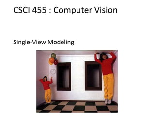
1. Single-View Modeling
CSCI 455 : Computer Vision

2. Single-View Modeling
• Readings
– Mundy, J.L. and Zisserman, A., Geometric Invariance in Computer Vision, Appendix:
Projective Geometry for Machine Vision, MIT Press, Cambridge, MA, 1992,
(read 23.1 - 23.5, 23.10)
• available online: http://www.cs.cmu.edu/~ph/869/papers/zisser-mundy.pdf
Ames Room

3. Roadmap ahead
• The next few lectures will finish up geometry
– Next up is recognition / learning
• We already know about camera geometry &
panoramas
• Coming up
– Single-view modeling (today)
– Two-view geometry
– Multi-view geometry

4. Ames Room
4

5. Projective geometry—what’s it good for?
• Uses of projective geometry
– Drawing
– Measurements
– Mathematics for projection
– Undistorting images
– Camera pose estimation
– Object recognition
Paolo Uccello

6. Applications of projective geometry
Vermeer’s Music Lesson
Reconstructions by Criminisi et al.

7. Making measurements in images

8. 1 2 3 4
1
2
3
4
Measurements on planes
Approach: unwarp then measure

9. Homogeneous coordinates and lines
• (X,Y,W) same as (SX,SY,SW)
• Line in projective plane
– ax + by + c = 0
– aX + bY + cW = 0
– uTp = pTu =0
• u = [a,b,c]T and p = [X,Y,W] T
• (x,y) Euclidean = (X/W,Y/W)
• W = 0? Ideal points, points at infinity (X,Y,0)

10. l
Point and line duality
– A line l is a homogeneous 3-vector
– It is  to every point (ray) p on the line: l.p=0
p1
p2
What is the intersection of two lines l1 and l2 ?
• p is  to l1 and l2  p = l1  l2
Points and lines are dual in projective space
l1
l2
p
What is the line l spanned by rays p1 and p2 ?
• l is  to p1 and p2  l = p1  p2
• l can be interpreted as a plane normal

11. Ideal points and lines
• Ideal point (“point at infinity”)
– p  (x, y, 0) – parallel to image plane
– It has infinite image coordinates
(sx,sy,0)-y
x-z image plane
Ideal line
• l  (a, b, 0) – parallel to image plane
(a,b,0)
-y
x
-z image plane
• Corresponds to a line in the image (finite coordinates)
– goes through image origin (principal point)

12. 3D projective geometry
• These concepts generalize naturally to 3D
– Homogeneous coordinates
• Projective 3D points have four coords: P = (X,Y,Z,W)
– Duality
• A plane N is also represented by a 4-vector
• Points and planes are dual in 3D: N P=0
• Three points define a plane, three planes define a point

13. 3D to 2D: perspective projection
Projection: ΠPp 




























1
****
****
****
Z
Y
X
w
wy
wx

15. Vanishing points (1D)
• Vanishing point
– projection of a point at infinity
– can often (but not always) project to a finite
point in the image
image plane
camera
center
ground plane
vanishing point
camera
center
image plane
ground plane

16. Vanishing points (2D)
image plane
camera
center
line on ground plane
vanishing point

17. Vanishing points
• Properties
– Any two parallel lines (in 3D) have the same vanishing
point v
– The ray from C through v is parallel to the lines
– An image may have more than one vanishing point
• in fact, every image point is a potential vanishing point
image plane
camera
center
C
line on ground plane
vanishing point V
line on ground plane

18. One-point perspective

19. Two-point perspective
vxvy

20. Three-point perspective

21. Questions?

22. Vanishing lines
• Multiple Vanishing Points
– Any set of parallel lines on the plane define a vanishing
point
– The union of all of these vanishing points is the horizon line
• also called vanishing line
– Note that different planes (can) define different vanishing
lines
v1 v2

23. Vanishing lines
• Multiple Vanishing Points
– Any set of parallel lines on the plane define a vanishing
point
– The union of all of these vanishing points is the horizon line
• also called vanishing line
– Note that different planes (can) define different vanishing
lines

24. Computing vanishing points
V
DPP t 0
P0
D

25. Computing vanishing points
• Properties
– P is a point at infinity, v is its projection
– Depends only on line direction
– Parallel lines P0 + tD, P1 + tD intersect at P
V
DPP t 0












































 
0/1
/
/
/
1
Z
Y
X
ZZ
YY
XX
ZZ
YY
XX
t
D
D
D
t
t
DtP
DtP
DtP
tDP
tDP
tDP
PP
 ΠPv
P0
D

26. Computing vanishing lines
• Properties
– l is intersection of horizontal plane through C with image plane
– Compute l from two sets of parallel lines on ground plane
– All points at same height as C project to l
• points higher than C project above l
– Provides way of comparing height of objects in the scene
ground plane
lC
v1 v2l

28. Fun with vanishing points

29. Lots of fun with vanishing points

30. Perspective cues

31. Perspective cues

32. Perspective cues

33. Comparing heights
Vanishing
Point

34. Measuring height
1
2
3
4
5
5.4
2.8
3.3
Camera height
How high is the camera?

35. q1
Computing vanishing points (from lines)
• Intersect p1q1 with p2q2
v
p1
p2
q2
Least squares version
• Better to use more than two lines and compute the “closest” point of
intersection
• See notes by Bob Collins for one good way of doing this:
– http://www-2.cs.cmu.edu/~ph/869/www/notes/vanishing.txt

36. Measuring height
without a ruler
H R

37. C
Measuring height without a ruler
ground plane
Compute Z from image measurements
• Need more than vanishing points to do this
Z

38. The cross ratio
• A Projective Invariant
– Something that does not change under projective
transformations (including perspective projection)
P1
P2
P3
P4
1423
2413
PPPP
PPPP


The cross-ratio of 4 collinear points
Can permute the point ordering
• 4! = 24 different orders (but only 6 distinct values)
This is the fundamental invariant of projective geometry













1
i
i
i
i
Z
Y
X
P
3421
2431
PPPP
PPPP



39. vZ
r
t
b
tvbr
rvbt


Z
Z
image cross ratio
Measuring height
B (bottom of object)
T (top of object)
R (reference point)
ground plane
HC
TBR
RBT


scene cross ratio














1
Z
Y
X
P











1
y
x
pscene points represented as image points as
R
H

R
H

R

40. Finding the vertical (z) vanishing point
Find intersection
of projections of
vertical lines

41. Measuring height
RH
vz
r
b
t
R
H
Z
Z



tvbr
rvbt
image cross ratio
H
vvx vy
vanishing line (horizon)
b0
t0

42. vz
r
b
vx vy
vanishing line (horizon)
t0
What if the point on the ground plane b0 is not known?
• Here the person is standing on the box, height of box is known
• Use one side of the box to help find b0 as shown above
b0
t1
b1
Measuring height
v
m0

43. 3D modeling from a photograph
St. Jerome in his Study, H. Steenwick

44. 3D modeling from a photograph

45. 3D modeling from a photograph
Flagellation, Piero della Francesca

46. 3D modeling from a photograph
video by Antonio Criminisi

47. 3D modeling from a photograph

48. Related problem: camera calibration
• Goal: estimate the camera parameters
– Version 1: solve for 3x4 projection matrix
ΠXx 




























1
****
****
****
Z
Y
X
w
wy
wx
• Version 2: solve for camera parameters separately
– intrinsics (focal length, principal point, pixel size)
– extrinsics (rotation angles, translation)
– radial distortion

49. Vanishing points and projection matrix









****
****
****
Π  4321 ππππ
1π 2π 3π 4π
 T
00011 Ππ  = vx (X vanishing point)
Z3Y2 ,similarly, vπvπ 
  originworldofprojection10004 
T
Ππ
 ovvvΠ ZYX
Not So Fast! We only know v’s up to a scale factor
 ovvvΠ ZYX cba
• Can fully specify by providing 3 reference points with known coordinates

50. Calibration using a reference object
• Place a known object in the scene
– identify correspondence between image and scene
– compute mapping from scene to image
Issues
• must know geometry very accurately
• must know 3D->2D correspondence

51. Chromaglyphs
Courtesy of Bruce Culbertson, HP Labs
http://www.hpl.hp.com/personal/Bruce_Culbertson/ibr98/chromagl.htm

52. AR codes
ArUco

53. Estimating the projection matrix
• Place a known object in the scene
– identify correspondence between image and scene
– compute mapping from scene to image

54. Direct linear calibration

55. Direct linear calibration
Can solve for mij by linear least squares
• use eigenvector trick that we used for homographies

56. Direct linear calibration
• Advantage:
– Very simple to formulate and solve
• Disadvantages:
– Doesn’t tell you the camera parameters
– Doesn’t model radial distortion
– Hard to impose constraints (e.g., known f)
– Doesn’t minimize the right error function
For these reasons, nonlinear methods are preferred
• Define error function E between projected 3D points and image positions
– E is nonlinear function of intrinsics, extrinsics, radial distortion
• Minimize E using nonlinear optimization techniques

57. Alternative: multi-plane calibration
Images courtesy Jean-Yves Bouguet
Advantage
• Only requires a plane
• Don’t have to know positions/orientations
• Good code available online! (including in OpenCV)
– Matlab version by Jean-Yves Bouget:
http://www.vision.caltech.edu/bouguetj/calib_doc/index.html
– Zhengyou Zhang’s web site: http://research.microsoft.com/~zhang/Calib/

58. Some Related Techniques
• Image-Based Modeling and Photo Editing
– Mok et al., SIGGRAPH 2001
– http://graphics.csail.mit.edu/graphics/ibedit/
• Single View Modeling of Free-Form Scenes
– Zhang et al., CVPR 2001
– http://grail.cs.washington.edu/projects/svm/index.htm
• Tour Into The Picture
– Anjyo et al., SIGGRAPH 1997
– http://www.mizuno.org/gl/tip/

59. Single-image depth prediction
Image Depth map
Deep
learning

60. Questions?