Thermo-Economic Frangopolus

1. Energy Vol. 12, No. 7, pp. 563-571, 1987 0360-5442187 $3.00 + 0.00
Printed in Great Britain Pergamon Journals Ltd
b,,
C
ce
CJ
CPY
&;h
km
f,
M
4
N
n3
“r
P
P
R.3
S
s
s
T
v
CL
x
Y
Y
Yr L
Yrk
Yr.,
THERMO-ECONOMIC FUNCTIONAL ANALYSIS AND
OPTIMIZATION
CHRISTOS A. FRANGOPOULOS
Department of Naval Architecture and Marine Engineering, National Technical University of
Athens, Athens 106 82, Greece
(Received 18 August 1986)
Abstract-Thermo-economic functional analysis is a method for optimal design or improvement
of complex thermal systems. Thermodynamic concepts are combined with economic considerations
in a systems approach. Units are the basic elements of the system; each unit has a particular
quantified function (purpose or product). The distribution of functions establishes inter-relations
between units or between the system and the environment and leads to a functional diagram of
the system. The optimization minimizes the total cost of owning and operating the system, subject
to constraints revealed by the functional diagram and analysis. The general formulation and a
numerical example are presented.
NOMENCLATURE
cost coefficients (constants) Greek letters
annual fixed charge rate ‘111 second-law efficiency
price of electricity (%/kJ) ‘lu = w/(,%?Ah) for the turbine-generator
price of fuel ($/kJ) = niAh/wfor the pump-motor
specific heat of water ). vector of all the Lagrange multipliers
chemical essergy of fuel 0 number of units
pump material factor (constant) T number of units and junctions
enthalpy per unit mass specific volume
number of outputs from unit r ; maintenance factor
mass w number of units, junctions and branching
number of inputs to unit r points
hours of operation per year
number of transfer units of condenser
number of decision variables for unit r
pressure
parameter
overall heat transfer resistance of condenser
entropy
negentropy
entropy per unit mass
temperature
velocity
power
vector of decision variables
contraint function
Subscripts
i the ith decision variable
0 reference state
r the rth unit (r = 0 is for the environment)
W water
Overmarks
per unit time
reference quantity (constant)
fixed value of an otherwise variable quantity
vector of all the inputs and outputs
the product of unit r
the kth output from r
thejth input to r
1. INTRODUCTION
Earlier work by Tribus, Evans and El-Sayed on thermo-economics’,’ led to the concept
of thermo-economic isolation (TI) introduced by Evans.3 In order to approach thermo-
economic isolation, Tribus’ and Evans et ~1.~made use of the functions or purposes of
thermal system components, but the conditions for approaching TI remained to be derived.
The attempt to derive formally the complete set of conditions for TI has led us to the
development of a new and generally applicable method for optimal design or improvement
of complex thermal systems, which we call thermo-economic functional analysis (TFA).’
2. FUNCTIONAL ANALYSIS
2.1 Concepts and definitions
A thermal system (thermal power plant, refrigeration plant, chemical plant, etc.) consists
of a set of inter-related units.6 Each unit has one particular function (purpose or product).
563
FRANGOPOULOS, Christos A. Thermo-economic functional analysis and optimization.
Energy, v. 12, n. 7, p. 563-571, 1987.

2. 564 CHRISTOSA. FRANGOPOULOS
Functional analysis is “the formal, documented determination of the function of the
system”7 as a whole and of each unit individually.5
2.2 The functional diagram ofa system
The picture of a system will be composed of small geometrical figures representing the
units and a network of lines representing the distribution of the unit functions. This is the
functional diagram of the system. Junctions (where the functions of two or more units
merge) and branching points (where the function of a unit is distributed to more than one
unit) are considered to be fictitious units, unless they correspond to real components of
the plant.
3. THERMO-ECONOMIC FUNCTIONAL OPTIMIZATION
The optimization objective is the minimization of the total cost of owning and operating
the system, with income included as a negative cost.
3.1 Total optimization
The system is considered to be operating at the steady state with products of a specific
type, but not necessarily of predetermined quantity. The objective function is
min P = i i, + lo? tO.k,
x r=l k=l
(1)
where p = cost rate of owning and operating the whole system, Z, = amortized capital
cost rate of unit r including fixed charges and maintenance, rO,k = cost rate associated
with yO.k. For 1 < k d 8O,p O,kis positive and represents expenditure corresponding to
services purchased by the system from the environment; penalties for environmental
pollution or other social hazards can be quantified and included. For
e,, + 1 Q k < !, + m,, rO,k is negative and represents profit from selling products.
Costs are functions of decision variables and quantities purchased or sold as follows:
z =Z,(X,,Yl,l) = z,, (24
pO.k = rO.k(YO.k) = rO.k, GW
P = F(x,y) = F. (W
Both sides of Eqs. (2) are expressions for cost rate, but the left hand side (e.g. Z,) represents
the cost rate quantity itself, while the right hand side (e.g. Z,) represents the mathematical
functional operation which generates its numerical value.
In view of Eqs. (2), the objective function takes the form
T$ F = i z,(x,? Y,.l) + “so rO.k(YO.k)~
r=l k=l
(3)
The equality constraints are
Y,,j = Y,,j(X,,Y,,l) E Y,,j (r = O,l,...,W i = L&...,m,L (4)
Y,~,~= yl,j (r’= O,l,..., w, k = 1,2,..., e,). (5)
The constraints (4) give the inputs to the unit I as functions of the product Y,.~and the
decision variables x, of the unit. The constraints (5) represent interconnections between

3. Thermo-economic functional analysis and optimization 5h5
units or between a unit and the environment, which are revealed by the functional diagram
of the system.
Inequality constraints would not alter the basic principles of the method, but they will
not be considered.
For the solution of the optimization problem, the method of Lagrange multipliers has
been chosen, which leads readily to the special cases of decomposition and thermo-
economic isolation.s The Lagrangian is
r=l k=l r=Oj=l
+ f f$A'.k(Yr,j- Yr’.k). (6)
r'=Ok=l
The necessary conditions for an extremum are
v,w, Y, J-1= 0, t7a)
V&(x, y,v =0, (7b)
V*L(x, y, k) = 0. (7c)
It is proved in Ref. 5 that the Lagrangian takes the convenient form
where
L= f err- i ir.kyr.k)+ f"i?rO.k - ju0.ky0.k)3
r=l k=l k=l
(8)
I-, = z, + t 4,jY.j.
j=I
(9)
The conditions (7~) lead to a restatement of the constraints given in Eqs. (4) and (5). The
conditions (7a, b) lead to
8
( >
i r, /fJX,i = 0 (r = 1,2,...,a, i = 1,2, ..., n,),
r=l
I 0.k= arO.k/dYO.k (k = 1,2 ,...) to + mo), (11)
&k = w~y,.k (r = 1,2 )“‘, 0, k = 1,2 ,..., t,). (12)
The concept of internal economy introduced by El-Sayed and Evans’ and the correspond-
ing interpretation of Lagrange multipliers as economic indicators of prices are maintained
here. According to Eqs. (1 I), (12), each Lagrange multiplier can be viewed as the marginal
price of the corresponding function (product) y.
The optimization problem is solved by using the following procedure: (a) select a set of
values for the decision variables x; (b) solve Eqs. (4), (5) for the dependent variables y; (c)
determine the Lagrange multipliers from Eqs. (1 l), (12). We stop when Eq. (10) is satisfied
to an acceptable approximation. Otherwise, we select a new set for x and repeat the
procedure.

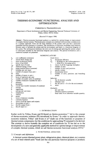
4. 566 CHRISTOSA. FRANGOPOULOS
3.2 Fixed-product optimization
This case arises when the income functions FO,(yc,J,
known, but the products are fixed and known quantities:
~O+l<k<to+mo, are not
Y0.k = 90,j (k = to+.i i = lg2,...,mo),
The objective function in such a situation is
(13)
minF = i Z,~,Y~J + ? ro.k(~o.k).
X,Y r=l k=l
(14)
Equation (6) is vaiid if the upper limit PO+ m, of the summation over I0.k is replaced by
lo, while Eq. (8) takes the form
>
+ ; (r0.k - l-O.kYO.k) + jtl ‘0.jfO.j
k=l
(15)
The procedure to solve the optimization problem is similar to the one described in Sec.
3.1.
3.3 Main actions for TFA and 0
In summary, the thermo-economic functional analysis and optimization of a thermal
system consists of the following actions: (1) identifying the functions of the system as a
whole and of each individual unit; (2) constructing the functional diagram of the system;
(3) formulating the optimization problem, i.e. (a) selecting the decision variables,(b) deriving
the cost functions ZI(x,, Y,.~)and &,k(yo.k), (c) deriving the constraint functions YI,Axr,y,,r),
(d) deriving the explicit form of the optimization equations; (4) solving the system of
optimization equations. Parametric study and sensitivity analysis may follow.
4. APPLICATION OF TFA AND 0 TO A FOUR-UNIT THERMAL POWER PLANT
4.1. Description of the plant and main assumptions
The method will now be applied to a simplified thermal power plant. The system is
considered to be made up of four units: (1) boiler, (2) turbine-generator, (3) condenser and
condensing supply works (e.g. cooling towers, coolinggwater-circulating pumps etc.), and
(4) boiler feed pump (see Fig. 1).
A distinction must be drawn between a unit and a component. The cooling tower or
cooling-water-circulating pump are components. However, in this example, they are not
considered to be separate units but are instead combined with the condenser in a unit
having one function. The number of units in a system is not unique and depends on the
available information and desired results. The designer may select high (many units) or
low resolution (a few units), depending on the objectives.
It is assumed that the plant produces only electrical power at a specified rate I& The
power required by the pump is supplied from outside the system. All of the components
are well insulated and losses through the pipes connecting the components are negligibly
small.
4.2. The functional diagram of the system
The function of each unit will be measured by means of essergy (as defined by Evans’)
and entropy. To identify the functions and their distribution, the following procedure is
used: a closed loop of an essergy-carrying stream is considered, Fig. 2. The units take from
this stream or from outside the system the amount of essergy required for their operation,

5. Thermo-economic functional analysis and optimization 567
Fuel
Ex.Gases Air
1.
I
C
1 - 1
I. _ -__-a
(a) *'"I
ti
w
Fig. 1. A four-unit thermal power plant (B = boiler, T = turbine, G = generator, C = condenser, P = pump).
and give their product either back to the stream or to the environment. The operation of
the units creates entropy, which is rejected to the environment through the condenser. In
other words, the condenser is supplying the system with the negative ofentropy, (negentropy,
as introduced by Brillouin’ and used by Smith” to quantify the function of the condenser).
A negentropy-carrying stream runs parallel to the essergy stream but in the opposite
direction (see Fig. 2).
yil.1
1,
r-
___---_--_-- -___
y1,1
1
y1,2
-J
1
y1,3
:
q.Yl.1
- _m5-*
r-- ,
s4
II
I . I,
1
.%,t .
5, 1
1 'IV1
I y2,1 /
y2.1
L2-2< 0
yod
Y2
I'
I
I
152
I
-_-_-
System Boundary
Fig. 2. The power plant with essergy and negentropy streams.
I

6. 568 CHRISTOSA.FRANGOPOULOS
I
i I t *5.1
L-,
I
i *2,i /
__~ r-;-eJ
y2.1
2-
----_ -L
" v
y2,2
7
L- -l-*3,2
_-____
-7---------
I l-*n :, System Boudary
Fig. 3. Functional diagram of a four-unit thermal power plant
Essergy and negentropy balances along each stream lead to expressions for the yr,j,
which are given in Appendix A. The concepts introduced in Sec. 2.2 and the procedure
described here lead to the functional diagram of the system (see Fig. 3).
An arrow pointing toward a unit does not necessarily represent a stream (of mass,
energy, essergy, etc.) entering the unit. For example, exhaust gases of a boiler form a stream
exiting the boiler; but, the service of getting rid of exhaust gases is provided to the boiler
by an other unit (not shown in Fig. 3, because of the resolution level selected). Similarly,
if the boiler is to be penalized for environmental pollution, then the corresponding
expenditure will depend on an appropriate measure of pollution, to be represented by an
arrow, say y1.4 pointing toward the unit.
4.3 Optimization of the system
Among the many quantities involved, the decision variables are selected to be
x = (q,rtrrl, T2, Gr~wt1,14). (16)
The remaining quantities are either dependent variables or parameters. The objective
function is given by Eq. (14) with CJ= 4 and /, = 3.
The procedure described at the end of Sec. 3.1 has been used to solve the optimization
problem for ri/= 20 MW. Figures 4 and 5 show the influence of fuel and electricity prices
on optimum values of decision variables. The effect of parameter uncertainties on the
optimum solution may be obtained by using sensitivity anaIysis. The change (uncertainty)
in the objective function due to a change (uncertainty) in a particular parameter may be
estimated from
AF = (dF/apj)Apj. (17)

7. Thermo-economic functional analysis and optimization 569
-6,Tb -h
(K) (K)
320 830
310
300
820
810
1.0 1.5 2.0 2.5 3.0 35 4.0
cF
(106$/d
Fig. 4. Effect of fuel price on optimum values of decision variables.
2.0 - - 0.84
;i
I%
'; 18- - 0.62 c2
>*
1.6 - - 0.60
1.4 - - 0.70
2 3 4 5 6 7
C,(C/kWhr)
Fig. 5. EfFect of electricity price on optimum values of decision variables.
The maximum possible uncertainty in the objective function caused by uncertainties in a
set of parameters is
AF,,, =
while the most probable uncertainty is
AF prob = J~C(aFlaPjWPjl’. (19)
(18)
As an example, sensitivity analysis results are presented in Table 1. Primarily economic
parameters have been selected, because of the inherent uncertainty in deriving or predicting
values of these parameters. Cost data found in the literature are only accurate to +25-
30%.

8. 570 CHRISTOSA. FRANGOPOULOS
Table 1. An example of sensitivity analysis
Parameter (pj)
j. aF
aPj
LIP!*’
3
AF.
Symbol Nominal Units 3
Value
1
=f
2.0x10-a B/kJ 7.7378x10C 2.0x10-' 1.5476x10-'
2 'e
8.33x1O-6 B/kJ 2.3541~10' 8.33x10-' 1.9610x10-'
3 bll 740. $/(kW)".8 3.7912x1o-5 74. 2.8055x10-'
4 b12 0.8 2.8941x10-1 0.08 2.3153x10-'
5 b21 3000. $/(kW)"*7 7.2855x10-' 300. 2.1857x10-:
6 b22 0.7 2.1645x10-l 0.07 1.5152x10-'
7 b31 217. S/m’ 1.2885~10-~ 21.7 2.7961x10-*
8 b32 577. S/(kg/s) 5.7447x1o-6 57.7 3.3147x1o-u
9 b41 378. $/(kW)".71 6.4086x10-' 37.8 2.4225x10-5
to b42 0.71 - 1.1835~10-~ 0.071 8.4O29x1O-5
Ll fm 1.06 - 5.3079x10-* 0.106 5.6264x10-'
L2 c 18.2 % 3.o914x1o-3 1.82 5.6264x10-j
AFmax
= 7.0940~10-* AF
prob
= 1.0813x10-'
(*) for Apj/pj = 0.10
Acknowledgements-The author expresses his sincere gratitude to R. B. Evans for advice and encouragement.
Support provided by the Georgia Institute of Technology and the National Technical University of Athens is
gratefully acknowledged.
REFERENCES
1. M. Tribus and R. B. Evans, A Contribution to the Theory of Thermoeconomics, UCLA Report No. 62-36,
University of California at Los Angeles, Los Angeles, Calif. (1962).
2. Y. M. El-Sayed and R. B. Evans, .I. Engng Power 92, 27 (1970).
3. R. B. Evans, Energy 5, 805 (1980).
4. R. B. Evans, W. A. Hendrix and P. V. Kadaba, Essergetic functional analysis for process design and synthesis,
in Ejiciency and Costing: Second Law Analysis ofProcesses (Edited by R. A. Gaggioli), p. 239. ACS Symposium
Series No. 235, Washington, D.C. (1983).
5. C. A. Frangopoulos, Thermoeconomic Functional Analysis: A Method for Optimal Design or Improvement
of Complex Thermal Systems. Ph.D. Thesis, Georgia Institute of Technology, Atlanta, Ga (1983).
6. N. J. T. A. Kramer and J. Smit, Systems Thinking: Concepts and Notions. Martinus Nijoff Social Sciences
Division, Leiden, The Netherlands (1977).
7. S. L. Dickerson and J. E. Robertshaw, Planning and Design. Lexington Books, Lexington, Mass. (1975).
8. R. B. Evans, A Proof that Essergy is the only Consistent Measure of Potential Work. Ph.D. Thesis, Dartmouth
College, Hanover, N.H. (1969).
9. L. Brillouin, Science and Information Theory, 2nd ed. Academic Press, New York (1962).
IO. M. S. Smith, Effect of Condenser Design upon Boiler Feedwater Essergy Costs in Power Plants. M.S. Thesis,
Georgia Institute of Technology, Atlanta, Ga (1981).
11. R. M. Garceau, Thermoeconomic Optimization of a Rankine Cycle Cogeneration System. M.S. Thesis,
Georgia Institute of Technology, Atlanta, Ga (1982).
12. J. G. Singer ed., Combustion: Fossil Power Systems, 3rd ed. Combustion Engineering Inc., Windsor, Conn.
(1981).
13. H. Popper, Modern Cost Engineering Techniques. McGraw-Hill, New York (1970).
14. R. S. Hall, J. Matley and K. J. McNaughton. Chem. Engng 89, 80 (1982).

9. Thermo-economic functional analysis and optimization 571
APPENDIX A
Expressions for the Functions of Fig. 2 and 3
The essergy flows related to the environment are:
y,., = $3 Y3.2 = fi,v,(P, - Pb)lVMW
~4.1 = ri/, = h(k, - hA/r7Md. y2, = ri/= ?/M*14?(hl- h2).
Other essergy flows are:
Y1.2 = fiv,(P* - PI), Y2.1 = M11/1 - (LA Y3.1 = Mti1 - $3).
Y4.1 = M+a - ti3)? L, = +, + Y4 , - Y1.2 = Mi, - v4(P4 - P,)l.
y, , ==9, - 9, = nicI(I1- $4)+ v4(P4 - P,)l,
where $ is the flow essergy per unit mass:
The negentropy flows are:
where:
$ = h - h, - T,(s - s,,) and 9” = ti$.
Y3.1 = $2 - $3 + y, 1 = Wl(s, - sj),
Y1.3 = $1 - $4 -+ y1.3 = ‘WAS, - &A
Y2,2 = $2 - $1 -+ y2.z = n;lT,(s, - s,),
Y4.2 = $4 - $3 -+ y4.2 = n;lT,(s, - s3).
S, = -nisi(i = 1,2,3,4)
The last forms of y3,,.y1 3,y2,2, and y4 z are obtained by multiplying negentropy flows by the reference
temperature To and changing the sign. This convenient procedure is used in order to obtain all functions as
positive quantities in the same units.
APPENDIX B
Cost Functions
The following equations have been derived in Ref. 5 by using information from several sources (e.g. Refs. 1I
14):
where:
i,, = (C/3.6 x 10SN)+,h,i, gP = expl(P, - ~,).!b,,l,
RI, = 1+ C(O,45 - ri,,,)/(O, 45 - %,P.
R,~= 1+ b,,exp[(T, - T,)/bJ(r = 1.2).
R,, = 1 + ~(1 - sdm - r7diVr = 2,4).