1. 1
2.STRESS STRAINS AND YIELD CRITERIA
Stress−Strain Relations
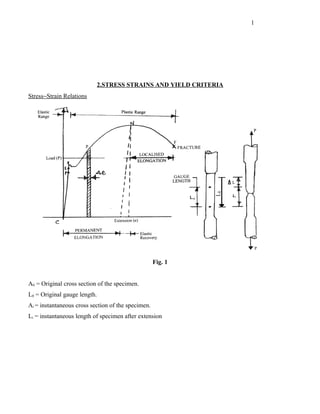
Fig. 1
A0 = Original cross section of the specimen.
L0 = Original gauge length.
Ai = instantaneous cross section of the specimen.
Li = instantaneous length of specimen after extension

2. 2
Fig. 2: Stress− Strain Diagram.
P = Proportionality limit E = Elasticity limit Y = Yield point
N = Necking Point F = Fracture Point
Fig. 3

3. 3
Fig. 4

4. 4
i. Engineering
Fi
Stress S = Fi = instantaneous load
A0
∆L Change in length  L − L0 
Engineering strain = = = 
L0 Original length of specimen  L0 
 
Fi
ii. True stress σ = and
Ai
Li
dL L 
True strain ∈ = ∫ = log  i 
L L 
L0  o 
True stress is defined as load divided by actual cross sectional area (not original cross sectional area
A0) for that particular load.
Fi
σ=
Ai
Similarly, true strain is based on the instantaneous specimen length rather than original length. As such
true strain (or incremental strain) is defined as
dL
d∈ = Where L is length at load F and ∈ is the true strain.
L
The true strain at load F is then obtained by summing all the increments of equation.
Arithmetically, this can be written as
dL0 dL1 dL2 dL3 dL
∈ = ∑d ∈ = + + + + ...... + n
L0 L1 L2 L3 Ln
L1
dL L1
= ∫ L
= log
L0
L0
True strain is the sum of each incremental elongation divided by the current length of specimen, where
L0 is original gauge length and Li is the gauge length corresponding to load Fi. The most important
characteristics of true−stress strain diagram is that true stress increases all the way to fracture. Thus true
fracture strength σ f is greater than the true ultimate strength σ u in contrast with engineering stress
where fracture strength is lesser than ultimate strength.

5. 5
Relationship between true and engineering stress strains
From volume constancy, V = A0 L0 = Ai Li
Li A
∴ = 0
L0 Ai
Li − L0  Li 
e= =  − 1
L0 L 
 0 
Li
∴ = ( 1 + e)
L0
Fi Fi A0 Li
σ= = × =S×
Ai A0 Ai L0
σ = S (1 + e)
Li
dL L
∈= ∫ = log i = log (1 + e)
L0
L L0
∴ ∈ = log (1 + e)
Problems with Engineering Stress−Strains
1. Engineering stress−strain diagram does not give true and accurate picture of deformation
characteristics of the material because it takes original cross sectional area for all calculations
though it reduces continuously after yield point in extension and markedly after necking. That’s
why we get fracture strength of a material less than its ultimate tensile strength is Su > Sf which is
not true.
2. Total engineering strain is not equal to sum of incremental strains which defies the logic.

6. 6
Let us have a specimen with length of 50 mm which then is extended to 66.55 in three steps
Length before extension (L0) Length after extension ∆L ∆L
E=
L0
0 50 50
1 50 55 5 5/50 = 0.1
2 55 60.5 5.5 5.5/55 = 0.1
3 60.5 66.55 6.05 6.05/60.5 = 0.1
5 5.5 6.05
Sum of incremental strain = + + = 0.1 + 0.1 + 0.1 =0.3
50 55 60.5
Now we will calculate total strain considering original and final length after of extension L3 = 66.55
L3 − L0 66.55 − 50
∴ Total engineering strain when extended = = = 0.331
L0 50
the specimen in one step
The result is that summation of incremental engineering strain is NOT equal to total engineering strain.
Now same procedure is applied to true strain-
 L L L 
∈ = ∈0−1 + ∈1−2 + ∈2 − 3 =  log 1 + log 2 + log 3 
 L0 L1 L2 
 
55 60.5 66.55
= log + log + log = 0.286
50 55 60.5
L3 66.55
But total true strain equals to ∈0.3 = log = log = 0.286
L0 50
In the case of true strains, sum of incremental strain is equal to the overall strain. Thus true strains are
additive. This is not true for engineering strains.
3.

7. 7
Fig
L0 = length before extension
L1 = L0 = length after extension
L1 − L 0 L1 − L 0
Strain e = ⇒ −I=
L0 L0
L1 = 0
Fig
To obtain strain of −1 the cylinder must be squeezed to zero thickness which is only hypothetical and
not true. Moreover, intuitively we expect that strain produced in compression should be equal in
magnitude but opposite in sign.
Applying true strain formulation, to extension
L1 2L 0
∈ = log = log = log 2
L0 L0
To compression; L1 = L0/2
L1 L0 / 2
∈ = log = log = log 1 / 2 = − log 2
L0 L0
gives consistent results. Thus true strains for equivalent deformation in tension and comprehension are
identical except for the sign. Further unlike engineering strains, true strains are consistent with actual
phenomenon.

8. 8
Problem:
The following data were obtained during the true strain test of nickel specimen.
Load Diameter Load Diameter
kN mm kN mm
0 6.40 15.88 5.11
15.30 6.35 15.57 5.08
15.92 6.22 14.90 4.83
16.32 6.10 14.01 4.57
16.5 5.97 13.12 4.32
16.55 5.84 12.45 3.78
A. Plot the true stress true strain curve:
B. Determine the following
1. True stress at maximum load.2.True fracture stress.3.True fracture strain.4.True uniform strain .
5. True necking strain. 6.Ultimate tensile strength.7. Strain hardening component.
Pmax 16.55 × 10 3
1. True stress at max load = = π = 617.77 MPa
A × 5.84 2
4
P 12.45 × 10 3
2. True fracture stress = = = 1109 MPa
A min 11.22
2 2
d 
3. True fracture strain = ln  0  = ln  6.4  = 1.053
 
d   3.78 
 i 
2 2
d   6.4 
4. True uniform strain = ln  0  = ln   =0.183
d   5.84 
 i 
5. True necking strain = true fracture strain −
true uniform strain = 1.053 − 0.183 = 0.87
Pmax 16.55 × 10 3
6. Ultimate tensile stress = = π = 514 MPa
A max × 6.4 2
4
7. Now, n= log(1+e) = log (1.2) =0.183

9. 9
Load Diamete Area True stress True strain = Engg. Stress Engg. Strain
KN r mm2 2
Pi d  P
mm ln  0  = d
2

= d  A = 0  −1
Ai  i  d 
 i 
2
(N/mm2)
(N/mm )
0 6.40 32.17 0 0
15.3 6.35 31.67 48.31 0.0156 475.59 0.0158
15.92 6.22 30.39 523.86 0.057 494.87 0.059
16.32 6.10 29.22 558.52 0.096 507.30 0.10
16.5 5.97 27.99 589.50 0.139 512.90 0.149
16.55 5.84 26,79 617.77 0.183 514.45 0.20
15.88 5.11 20.5 774.63 0.45 493.62 0.568
15.57 5.08 20.27 768.13 0.46 484.00 0.587
14.90 4.83 18.32 813.32 0.56 463.16 0.755
14.01 4.57 16.40 854.27 0.67 435.5 0.961
13.12 4.32 14.66 894.95 0.786 407.83 1.19
12.45 3.78 11.22 1109.63 1.053 387.00 1.866
Applications of Engineering Stress and Strains
Engineering stress and strain are useful for many engineering design applications. Computation of
stress and strain is based on initial area or gauge length and therefore engineering stress and strain
represent only approximations of the real stress and strain in plastic zone.
In elastic deformation region (where dimensional changes are small and negligible) the initial and
instantaneous areas are approximately same and hence true stress equals engineering stress. Therefore,
in design problems where large dimensional changes do not occur, the use of engineering stress is
sufficiently accurate and used extensively as it is easier to measure.
However, for metal working where large plastic deformations occur and are necessary, the
approximations inherent in engineering stress and strain values are unacceptable. For this reason, the
true stress and true strains are used.
Important advantages of true stress−strain curves:
1. It represents the actual and accurate stress and strain. True strain refers to a length from
which that change is produced rather than to original gauge length.The engineering stresse and

10. 10
strains provides incorrect values after yield point i.e. plastic zone which a main zone of interest for
metal working.
2. True strains additive i.e. the total overall strain is equal to sum of incremental strains.
3. True strains for equivalent deformation in tension and compression are identical except in sign.
4. The volume change is related to the sum of the three normal true strains and with volume constancy.
5. True stress can be related to true strain.
σ = K (∈) n σ = (∈0 + ∈) n
∈0 = the amount of strain hardening that material received prior to the tension test.
6. True−stress−true strain values are quite sensitive to change in both metallurgical and mechanical
conditions of matter.
True−stress−strain Engineering
1. Actual values of gauge length and 1. Original cross sectional areas (A0) is
cross sectional area is used in used for calculating engineering stress.
calculating true stress and true strain. Fi
S=
Li A0
Fi dL
σ= ∈= ∫
Ai L0
L Li − L0
Further strain e = is used.
L0
The sum of incremental strains is
The sum of incremental strains is not
equal to total strain
equal to total strain.
Unlike load elongation curve, there is
no maximum in the true strin curve.
The sloppe of the curve in the plastic
region decreases with increase in
strain
2. The calculated values of stress− 2. The nominal stress (s) defined for the
strain are real and very useful in the tensile test in terms of original cross
plastic region of the curve. sectional area (A0) is not really stress
because the cross sectional area Ai at
the instant of load measurement is less
than A0 in the evaluation of s.
3. The metal working designers are 3. The structural designers are interested
interested in plastic region where in a region where strains are elastic

11. 11
difference between Ai and A0 is and difference between Ai and A0 is
significant. The true stress−strains negligibly small. But this is not true in
give accurate picture and hence it is the plastic region and especially when
more useful to metal working designs. maximum load is reached.
4. It is not easy to obtain values of σ 4. It is easy to obtain these values
from test since the force Fi and cross through test and convenient−less
sectional area (Ai) must be measured costly. These values are widely
simultaneously. True stress ( σ ) is available and documented.
important in metal working
calculation because of its
fundamental significance.
5. It is more consistent with the 5. It is less consistent with physical
phenomenon of metal deformation. phenomenon of metal deformation.
Idealisation of stress – strain curves
The solutions to the plasticity problems are quite complex. To obtain solution to these problems,
stress – strain curves are idealized by [i] neglecting elastic strains and/or [ii] ignoring the effect work
hardening. Idealization and simplification restrict its field of application.
1. Elastic perfectly plastic
It considers elastic strains and neglects effects of work hardening; it yields more difficult constitutive
relations. As a consequence, it also leads to greater mathematical difficulties in practical applications.
It must be used for those processes in which elastic and plastic strains are of the same order. This is the
case in structural engineering or for bending.
2. Rigid, perfectly plastic
In most metal forming operations, the permanent strains are much longer than the elastic. One therefore
in air no great error by assuming the metal to behave as a rigid body prior to yielding. It is for this
reason that one mainly employs perfectly plastic material idealisation.

12. 12
(a) Perfectly elastic, brittle (b) Perfectly rigid plastic
(c) Rigid, linear strain hardening (d) Elastic – perfectly plastic
(e) Elastic – linear strain hardening
Fig. 5
The flow curve
A true stress–strain curve is frequently called a flow curve because it gives the stress required to cause
the metal to flow physically to given strain.
The plastic region of a true stress – strain curve for many materials has a general form in the form of
Holloman equation which is
σ = k (∈) n
where: n is strain hardening exponent

13. 13
k is strength constant
Fig. 6
In a tension test of stell, a specimen of circular cross section with original diameter 9 mm is used. The
loads applied were 22 kN and 28 kN which reduces its diameter to 8.6 mm and 8.3 mm respectively.
Determine (i) true stress and true strain for given loads (ii) strain hardening exponent and strength
coefficient.
Solution:
d 0 = original diameter of specimen = 9 mm
d1 = diameter of specimen on application of load F1 = 22kN
d 2 = diameter of specimen on application of load F2 = 28kN
F1 22 × 10 3 ( N)
σ1 = = = 3.78 N / mm 2
2
π / 4 d1 π / 4 (8.6) 2
F2 28 × 10 3
T2 = = = 517.5 N / mm 2
π / 4 (8.3) 2 π / 4d2
2
L1
∈= true strain = log e
L0
L1 = Length after deformation
L 0 = length before deformation

14. 14
As volume of specimen remain constant,
A 0 × L 0 = A1 × L1
2
π 2 π 2 L1 d 
d 0 × L 0 = d1 × L1 ∴ = 0 
4 4 L 0  d1



2
d  d
∴ ∈= log  0
d  = 2 log 0

 1  d1
∈1 = true strain for first extension
9
∴ 2 log = 0.091
8 .6
∈2 = true strain for second extension
d 9
= 2 log 0 = 2 log = 0.1619
d1 8.3
Applying Hollomon equation,
n
σ1 = K∈1
σ 2 = K ∈n
2
n σ ∈
σ2 ∈ 
∴ = 2  or log 2 = n . log 2
σ1  ∈1 
  σ1 ∈1
σ 517.5
log 2 log
n= σ1 = 378 = 0.54
∴
∈2 0.1619
log log
∈1 0.091
Substituting the value of ‘n’ in equation (1)
378 = k (0.091) 0.54
K = 1385 N / mm 2

15. 15
∴ strain hardening exponent (n) = 0.54
strength coefficient K = 1385 N / mm 2
with this information, Hollomon equation can be written as
σ = 1385 (∈) 0.54
Both n and K are material properties: The strain hardening exponent physically reflects the rate at
which the material hardens. The derivative of this equation
dσ  d ∈
= n
 ∈ .

σ  
In states that fractional change in true stress caused by a fractional change in true strain is determined by
the strain hardening exponent (n). Therefore, the stress increases rapidly with strain for a material that
has a large strain hardening exponent, such as 3O 2 stainless steel (n = 0.3) compared to a material
where n is low such as 4.10 stainless steel (n = 0.1).
Plastic Instability
Necking or localised deformation begins at maximum load where decrease in cross sectional area
which hears the load is compensated by increase in strength due in load
dF = 0

16. 16
Fig. 7
F = σ.A
dF = σ dA + A dσ = 0
dA dσ
⇒ − =
A σ
From constancy of volume, V = A . L A= cross section of spearmen
L =
length of specimen
dV = 0 = A. dL + dA L
dA dL
∴ − =
A L
dσ dl
∴ = = d∈
σ L
dσ
∴ =σ
d∈
Problem
Prove that uniform strain is equal strain hardening exponent (n).
Solution:

17. 17
Fig.
P = load at any instance
A = cross section of specimen.
P = A σ = A . k (∈) n σ = k (∈) n (1)
Ao A
∈ = log ∴ e∈ = 0
A A
⇒ A = A 0 e −∈ (2)
Substituting value in equation (1)
P = A 0 e −∈ K (∈) n
P = K A 0 [e −∈ (∈) n ]
At maximum load point on engg.
stress – strain curve dP = 0
∈ = ∈u
When true strain
dP = K A 0 [e −∈N (∈u ) n −1 + (−1) e −∈ ∈u n ] = 0
n ∈u n −1 =∈u n
∴
∈u = n
Problem 1:
Hollomon equation for a material is given as σ = 1400 (∈) 0.33 . Find the ultimate tensile strength of the
material.
Solution:

18. 18
Ultimate tensile strength of a material is measured at maximum load point and where necking begins.
Upto the necking point, deformation is uniform throughout its gauge length. It is a engineering stress
(S u ).
True strain for uniform elongation is equal to strain hardening exponent. Therefore ∈u = n.
σu
Ultimate tensile strength = = S u = [σ = (1 + e) × S]
1 + σu
∈u = log e (1 + e u )
∴ ∈u = (1 + e u )
e = 2.71 (logarithmic base)
1 + eu = en
n n
σu K . ∈u n ∈ n 
∴ Su = = = K u  = K n 
 
 e  e
en en    
=
0.33
 0.33 
1400 
 2.71 
 = 698.1 N / mm 2
 
∴ UTS = 698. 1 N / mm 2
This shows that ultimate strength of a material can be calculated from the value of K and n.
Problem 2:
A metal obeys Hollomon relationship and has a UTS of 300 MPa. To reach the maximum load requires
an elongation of 35%. Find strain hardening exponent (n) and strength coefficient (K).
Solution:
UTS = S u = 300 MPa = 300 N / mm 2
Engineering elongation strain = e u = 35% = 0.35

19. 19
uniform true strain ∈u = log (1 + e u ) = log (1.35) = 0.3
σ u = S u (1 + e u ) but n = ∈u = 0.3
= 300 (1 + 0.35) = 405 N / mm 2 .
σ u = K (∈u ) n = k (n ) n
405 = K (0.3) 0.3
∴ K = 581.2 N / mm 2
∴ Hollomon equation for given metal is
σ = 581.2 (∈) 0.3
Deformation work
Work is defined as the product of force and distance. A quantity equivalent to work per unit volume is
the product of stress and strain. The area under the true stress strain curve for any strain ∈1 is the energy
per unit volume (u) or specific energy, of the deformed material.
Fig. 9
∈1
u = ∫σ d∈
0

20. 20
The true stress–strain curve can be represented by the Hollomon equation σ = K (∈) n .
∈1 ∈1
K ∈n +1
n
u = ∫ K (∈) . d ∈ =
0
n +1
0
K ∈1n +1
u=
n +1
similarly mean flow stress can be found
∈1 ∈1
n
∫σ d∈ ∫ K ∈ .d ∈
K ∈1n +1 K ∈1n
0 0
σm = = = =
∈1 −0 ∈1 (n + 1) ∈1 (n + 1)
K ∈1n
σm =
n +1
The work calculated according to above equation assumes that the deformation is homogeneous through
out the deforming part. This work is called ideal deformation work.
Example: Ideal work of deformation
Deformation of fully annealed AA–1100 aluminium is governed by the Hollomon equation. If a 10 cm
long bar of this material is pulled in tension from a diameter of 12.7 mm to a diameter of 11.5, calculate
the following:
a. the ideal work per unit volume of aluminium required;
b. the mean stress in the aluminium during deformation;
c. the peak stress applied to the aluminium.
σ = 140 (∈) 0.25 N / mm 2
Solutions
a. Calculate total strain during deformation

21. 21
A0 d
∈ = ln = 2 ln 0
A d
12.7
= 2 ln = 0.199
11.5
Calculate the total volume of bar
πd2 π (0.0127 m 2
V= ×l= × 0.1 m = 1.26 × 10 − 5 m 3
4 4
For AA–1100, K = 140 MPa and n = 0.25. Note that, as ∈< n, the deformation is homogeneous
∈1 +1
n
Wi = K × ×V
n +1
1.25
= 140 × 10 6 N × 0.199 × 1.26 × 10 − 5 m 3 = 187.5 N (J )
m 6 1.25
(b) Mean stress during deformation
n
∈1
σm = K ×
n +1
0.199 0.25
= 140 MPa × = 74.8 MPa
1.25
(c) Peak (maximum) stress applied, from Hollomon equation
σ1 = K ∈1 = 140 MPa × 0.199 0.25 = 93.5 MPa
n
Yield Criterion
Yield point under simplified condition of uniaxial tension is widely known and documented. But such
simplified conditions [1 – Pure uniaxial tension 2 – Pure shear] are rare in reality. In many situations
complex and multiaxial stresses are present and in this situation it is necessary to know when a material
will yield. Mathematically and empirically, the relationships between the yield point under uniaxial
tensile test and yield strength under complex situations have been found out. These relationships are
known as yield criteria. Thus yield criterion is defined as mathematical and empirically derived

22. 22
relationship between yield strength under uniaxial tensile load and yielding under multiaxial complex
stress situation.
Yield Criterion is a law defining the limit of elastic behaviour under any possible combination of
stresses is called yield criterion. Yield criterion is a mathematical expression which unites experimental
observations with mathematical expressions n a phenomenological manner. Yield criteria is primarily
used to predict if or when yielding
will occur under combined stress states in terms of particular properties of the metal being stressed [
σ 0 , K] .
Any yield criterion is a postulated mathematical expression of the stress that will induce yielding or the
onset of plastic deformation. The most general form is
f (σ x , σ y , σ z, Txy , Tyz , Tzx ) = a constant.
or in terms of principal stresses
f( f (σ1 , σ 2 , σ 3 ) = C
For most ductile metals that are isotropic, the following assumptions are invoked:
1. There is no Bauschinger effect, thus the yield strengths in tension and compression are equivalent.
Bauschinger effect
The lowering of yield stress for a material when deformation in one direction is followed by deformation
in the opposite direction, is called Bauschinger effect.

23. 23
Fig. 10
2. The constancy of volume prevails so that plastic equivalent of poison’s ratio 0.5.
σ1 + σ 2 + σ 3
3. The magnitude of the mean normal stress σ m = does not cause yielding. The
3
assumption that yielding is independent of σm (also called hydrostatic component of the total state
of stress) is reasonable if plastic flow depends upon shear mechanism such as slip or twinning. In
this context, yield criterion is written as
F[(σ1 − σ2), (σ2 − σ3), (σ3 − σ1)] = C
which implies that yielding depends upon the size of the Mohr’s circle and not their position. It is
shown that if a stress state (σ1, σ2, σ3) will cause yielding, an equivalent stress state
(σ1′ , σ 2 ′ , σ 3′ ) will cause yielding, if,
Two widely used yield criterion:
1. Tresca criterion or maximum shear stress criterion.
2. Von Mises criterion or distortion energy criterion.
1. Tresca criterion
Tresca found that plastic flow in a metal begins when tangential stress attains a value.
Assume that a body is subjected to triaxial stresses. σ1 , σ 2 , σ 3 are principal stresses and σ1 > σ 2 > σ 3
(algebraically).
Then maximum shear stress
σ − σ3
Tmax = 1
2
when Tmax exceeds a certain value ‘c’, specific to that material, yielding will occur. To find the value
of ‘c’, the material is subjected to uniaxial tensile test and find out yield point strength (σ 0 ).

24. 24
For uniaxial tensile test, stress situation is
σ1 = σ 0 , σ 2 = σ 3 = 0
σ − σ3 σ 0
∴ Tmax = 1 = =c
2 2
σ − σ3 σ0
∴ 1 = or σ1 − σ 3 = σ 0
2 2
ii) Material is subjected to pure shear:
σ1 = k σ2 = 0 σ 3 = −k k = shear strength of the material
σ1 − σ 3 = σ 0
∴k + k = σ0
σ
k = 0 = 0.5 σ 0
2
Application:
i) Plain stress condition. σ x , σ y, Txy
2
σx + σy  σx + σy 
σ1 = +   + (T ) 2
2  2  xy
 
2
σx + σy  σx + σy 
σ2 = −   + (T ) 2
2  2  xy
 
∴ σ1 = σ 0 when σ 3 > 0
σ1 + σ 3 = σ 0 when σ 3 < 0
ii) Plain strain condition ∈3 = 0 σ 2 = 2 (σ1 + σ 2 )
σ + σ3
σ1 − σ 3 = σ 0 σ2 = 1
2

25. 25
Shortcomings
1. An essential short coming of this criterion is that it ignore the effect of intermediate principal stress
(σ 2 ).
2. Since pastic flow depends upon slip phenomenon which is essentially a shearing. Slip is
practically absent in brittle materials. Therefore application of this criterion is limited to ductile
materials. This criterion is not applicable to crystalline brittle material which cannot be brought
into plastic state under tension but yield a little before compress fracture in compression.
3. Failure of/ yielding of a material under triaxial pure tension condition where σ1 = σ 2 = σ 3 can not
be explained by this criterion.
4. It suffers from a major difficulty that it is necessary to know in advance which are maximum and
minimum stresses.
5. Moreover, the general form of this criterion is far more complicated than the Von Mises criterion.
Therefore Von Mises criterion is preferred in most theoretical (not practical) work.
For sake of simplicity, in analysis, this criterion is widely used in practice.

26. 26
Von Mises Criterion
According to this criterion, yielding will occur when shear strain energy per unit volume reaches a
critical value. The shear strain energy per unit volume is expressed terms of three principal stresses:
e=
1
σG
[
(σ1 − σ 2 ) 2 + (σ 2 − σ 3 ) 2 + (σ 3 − σ1 ) 2 ]
G = modulus of shear which is a constant.
(σ1 − σ 2 ) 2 + (σ 2 − σ 3 ) 2 + (σ 3 − σ1 ) 2 = Constant.
(i) For uniaxial tensile test, yielding will occur when σ1 = σ 0 ; σ 2 = σ 3 = 0
(σ y ) 2 + (−σ y ) 2 = cons tan t = 2 σ 0 2
Therefore Von Mises criterion can be stated as
(σ1 − σ 2 ) 2 + (σ 2 − σ 3 ) 2 + (σ 3 − σ1 ) 2 = 2 σ 0 2
(σ x − σ y ) 2 + (σ y − σ z ) 2 + (σ z − σ x ) 2 + σ (T 2 + T 2 + T 2 ) = 2σ 0 2
x y y z z x
i) For plane stress: σ 2 = 0
σ + σ3
ii) For plane strain: σ 2 = 1
2
iii) For pure shear stress condition:
σ1 = k σ2 = 0 σ 3 = −k
(σ1 − σ 2 ) 2 + (σ 2 − σ 3 ) 2 + σ 3 − σ1 ) 2 = 2 σ 0 2
(k 0 − 0) 2 + (0 + k 0 ) 2 (− k 0 − k 0 ) 2 = 2 σ 0 2
σ k 02 = 2 σy2
σy
∴k = = 0.557 σ 0
3

27. 27
This is the relationship between shear yield strength and tensile yield strength of the material as per Von
Mises criterion.
k = 0.5 σ 0 2 Tresca criterion
k 0 = 0.577 σ 0 Von Mises criterion.
σy
Von Mises criterion satisfy the experimental data better than Tresca and therefore k = value is
3
normally used.
Advantages of Von Mises criterion
1. It overcomes major deficiency of Tresca criterion. Von Mises criterion implies that yielding is not
dependent on any particular normal stress but instead, depends on all three principal shearing
stresses.
2. Von Mises criterion conforms the experimental data better than Tresca and therefore more
realistic.
3. Since it involves squared terms, the result is independent of sign of individual stresses. This is an
important since it is not necessary to know which is the largest and the smallest principal stress in
order to use this criterion.
Von Mises yield criteria:
[(σ x − σy )
2
+ (σ y − σ z ) 2 + (σ z − σ x ) 2 + 6 (T 2 xy + T 2 yz + T 2 zx ) = 2 σ 0 2 ]
Effective stress
With the yield criterion, it is useful to define an effective stress denoted as σ which is function of the
applies stresses. If the magnitude of σ reaches a critical value, then the applied stress will cause
yielding.
For Von Mises criterion
σ=
1
2
[(σ1 − σ2 )
2
+ (σ 2 − σ 3 ) 2 + (σ 3 − σ1 ) 2 ] 1/ 2

28. 28
For Tresca criterion
σ = σ1 − σ 3
σ ≥ σ 0 ……………………. For both the criteria.
σ ≥ 3 k …………………. Von Mises
σ ≥ 2 k …………………… Tresca
Plane stress condition Plane strain condition
1. In plane stress condition, there is no stress 1. In plane strain condition, the strain
in third direction is absent.
in third direction.
1
∈2 = [ σ 2 − υ(σ 3 + σ1 )]
E
∴ σ 2 = υ ( σ1 + σ 3 )
Near yield point and in plastic zone
1
υ = (For plastic defo)
2
 σ + σ3 
σ2 =  1 
But there is strain in third direction. Two  2 
principal stresses
2
σx + σy  σx + σy 
σ1 =
2
+ 
 2
 + Txy 2
 ( )
 
2
σx + σy  σx + σy ) 
σ2 =
2
− 
 2  ( )
 + Txy 2
 
1
∈1 = [ σ1 − υ (σ 2 )]
E
1
∈2 = [ σ 2 − υ (σ1 )]
E
1
∈3 = [ 0 − υ (σ1 + σ 2 )]
E
Plane strain condition

29. 29
In majority of metal forming operations the problem can be simplified by assuming a condition of plane
strain is one. One of the principal strains is zero.
1
∈1 = [ σ1 − υ (σ 2 + σ 3 )]
E
1
∈2 = [ σ 2 − υ (σ1 + σ 3 )]
E
1
∈3 = [ σ 3 − υ (σ1 + σ 2 )]
E
let ∈2 = 0 ⇒ σ 2 = υ (σ1 + σ 3 ) for plastic region, Nadai has shown that υ = 0.5
 σ + σ3 
σ2 =  1 
 2 
σ + σ3
Thus, for Tresca criterion: σ1 , 1 , σ3
2
σ1 − σ 3 = σ 0
Von Mises criterion in plane strain:
2 2
 σ + σ3   σ + σ3 
 σ1 − 1  + 1 − σ 3  + (σ 3 − σ1 ) 2 = 2 σ 0 2
 2   2 
3
( σ1 . σ 3 ) 2 = 2 σ 0 2
2
 2 
 σ1 − σ 3 ) 2 =
 σ 0 = σ '0 

 3 
σ '0 = 1.155 σ 0 = constrained yield strength of the material.

30. 30
Yield criterion
Maximum shear stress Maximum distortion
Criterion (Tresca) energy criterion (Von Misces)
Plane Plane Pure
Stress Strain Shear
σ + σ2
σ 2 − 0, σ min = σ 2 σ= 1 σ1 = −σ 3 = k σ 2 = 0
2
σ1 = σ 0 .....σ 3 = ⊕ ve σ1 − σ 3 = σ 0 σ1 + σ 3 = σ 0
σ1 + σ 3 = σ 0 σ 3 = Οve 2k= σ0
σ0
k=
2
Plane stress Plane strain Pure Shear
σ1+σ3 1
σ12 + σ 3 2 − σ1σ 3 = σ 0 2 σ2 = k= σ0
2 3
2
σ1 − σ 3 = σ0
3
Tresca criterion Von Mises yield criterion
1. This criterion is also known as 1. Van Mises criterion is also known as
maximum shear stress criterion and distortion energy yield criterion. It states
attributes yielding to slip that yielding occurs when deformation
phenomenon which occurs when energy per unit volume of material
maximum shear stress exceeds a exceeds certain value which is
value, characteristic to the material. characteristic of the material.
Mathematically it can be stated as Mathematically, it can be stated as

31. 31
σ1 − σ 3 = σ 0
σ0 =
1
[(σ 1 − σ2 )
2
+ (σ 2 − σ 3 ) 2
]
2
where σ1, σ 2 , σ 3 are principal
+ (σ 3 − σ1 ) 2 1 / 2
stresses, and σ1 > σ 2 > σ 3 .
Or
1 
σ0 = (σ − σ y ) 2 ) 2 + (σ y − σ z ) 2
 x
2
+ (σ z − σ x ) 2 +
σ (τ 2 xy + τ 2 yz + τ 2 zx ) ] 1/ 2
2. Phenomenon of slip is limited to 2. The application of this yield criterion
ductile materials and hence holds good for both ductile and brittle
application of this criterion is limited materials.
to ductile materials. This criterion do
not yield good results for brittle
materials.
3. Tresca criterion ignores the effect of 3. Von Mises criterion take into considera−
intermediate principal stress and this tion the intermediate principal stress and
is a major draw back of this. hence move realistic. The predications
offered by Von Mises criterion conforms
empirical data.
4. 4. The yield stress predicted by Von Mises
criterion is 15. 5% greater than the yield
stress predicted by Tresca criterion.
5. Locus shown in Figure. 5. . Locus shown in Figure.
It is Hexagonal. It is Elliptical.

32. 32
Superimposed
6. Von Mises criterion is preferred where
6. Tresca criterion is preferred in
more accuracy is desired.
analysis for simplicity.
Locus of yield as per Tresca criterion
Biaxial stress condition is assumed to present locus of yield point on plane paper.
σ1 , σ 3 , σ2 = 0
yielding will occur if the point plotted is on the boundary or outside.

33. 33
Fig. 11 : Tresca yield locus. In the six sectors, the following conditions apply:
I σ 3 > σ1 > 0, so σ 3 = + Y II σ 3 > σ1 > 0, so σ 3 = + Y
III σ1 > 0 > σ 3 , so σ1 − σ 3 = + Y IV 0 > σ1 > σ 3 > 0, so σ 3 = − Y
V 0 > σ 3 > σ1 , so σ1 = − Y VI σ 3 > 0 > σ1 , so σ 3 − σ1 = + Y
Locus of yield as per Von Mises criterion
1. For a biaxial plane stress condition (σ 2 = 0) the Von Mises criterion can be expressed
mathematically,
σ12 + σ 3 2 − σ1σ 3 = σ 0 2
This the equation of an ellipse whose major semiaxis is 2 σ 0 and whose minor semiaxis is
2
σ 0 . The plot of equation is called a yield locus.
3

34. 34
Fig. 12
Comments
1. Yielding will occur if the point representing the given stress is plotted and is on the boundary or
outside the boundary.
2. The yield locus of maximum shear stress criterion [Tresca criterion] fall inside the maximum
distortion energy criterion [Von Mises] yield locus.
3. Two yield criteria predict the same yield stress for conditions of uniaxial stress and balanced
biaxial stress (σ1 = σ 3 ). The greatest divergence between the two criteria occurs for pure shear
(σ1 = −σ 3 ).
4. The yield stress predicted by the Von Mises criterion is 15.5% greater than the yield stress,
predicted by Tresca criterion.
Derive a mathematical expression for Von Mises yield criterion applicable to plane strain stress
condition:
Solution:
Von Mises yield criterion is stated as
(σ1 − σ 2 ) 2 + (σ 2 − σ 3 ) 2 + (σ 3 − σ1 ) 2 = 2 σ 0 2
where σ1 , σ 2 , σ 3 are three principal stresses and σ 0 is the yield strength of material. In plane strain
stress condition, the intermediate principal stress is arithmetic mean of other two. Assuming
σ1 > σ 2 > σ 3 , we can write
σ + σ3
σ2 = 1
2
substituting the value of σ 2 in the above expression
2 2
 σ + σ3   σ + σ3 
 σ1 − 1  + 1 − σ 3  + ( σ 3 − σ1 ) 2 = 2 σ 0 2
 2   2 

35. 35
(σ1 − σ 3 ) 2 (σ1 − σ 3 ) 2 (σ 3 − σ1 ) 2
+ + = 2 σ02
4 4 1
σ (σ1 − σ 3 ) 2
= 2 σ02
4
(σ1 − σ 3 ) 2 = 8 / 6 σ 0 2
2
∴ σ1 − σ 3 = σ0 = σ0'
3
σ 0 ' is called constrained strength of material and is 1−15 times the yield strength under uniaxial tensile
test.
PROBLEM
A stress analysis of a space craft structural member gives the state of stress as below:
200 30 0 
 
Tij =  30 100 0 
 0
 0 − 50

If the part is made of aluminium alloy with strength 500 MPa, will it exhibit yielding as per Tresca yield
criterion and von Mises yield criterion? If not, what is the safety factor?
Data given:
σ x = 200 MPa
σ y = 100 MPa
σ z = − 50 MPa
Tx y = 30 MPa
(1) Applying von Mises criterion
1/ 2
1 
2
σc =
2
( ) ( )
 σ x − σ y 2 + σ y − σ z 2 + (σ z − σ x ) 2 + 6  T 2 − T 2 + T 2  

 x y y z

z x 
 

36. 36
( )
1/ 2
1 
( 200 − 100) 2 + (100 + 50) 2 + ( − 50 − 200) 2 + 6 30 2 + 0 2 + 0 
2
σc =  
2  
∴ σ c = 224 MPa
The calculated stress ( σ c ) is less than the yield strength of the material (σ 0 ) , yielding will not occur as
per von Mises criterion
σ0 500 MPa
Factor of safety = = = 2.2
σc 224 MPa
(ii) Applying Tresca Criterion
In order to apply this criterion, it is necessary to know the magnitude and sign of three principal
stresses stress situation can be written in matrix form.
σ Txy Txz  200 30 0 
 x   
Tij = Tyx σy Tyz  =  30 100 0 
T Tzy σz   0 0 − 50
 zx   
20 3 0 
 
=  3 10 0  × 10
 0 0 − 5
 
To find the principal stresses σ
20 − σ 3 0
3 10 − σ 0 =0
0 0 − 5−σ
∴ I1 = σ x + σ y + σ z = 20 + 10 − 5 = 25
σx Txy σy Tyz σx Txz
I2 = + +
Txy σy Tyz σz Txz σz
= 191 − 50 − 100

37. 37
∴ I2 = 41
I 3 = Tij
10 0 3 0 3 10
= 20 −3 +0
0 −5 0 −5 10 0
= − 1000 + 45
∴ I3 = − 955
f (σ) = σ 3 − I1σ 2 + I 2 σ − I 3 = 0
σ 3 − 25 σ 2 + 41 σ + 955 = 0
Applying standard method to get cubic roots,
f (σ) = σ 3 − 25 σ 2 + 41 σ + 955 = 0
f(y) = y3 + py2 + qy + r = 0
∴ p = − 25
q = 41
r = 955
a=
1
3
( 1
)
3q − p 2 = ( 3 × 41 − 625)
3
a = − 167.3
b=
1
[
27
2p 3 − 9 pq + 27r ]
=
1
27
[2(−25) 3
− 9(−25) ( 41) + 27(955) ]
∴ b = 139.25

38. 38
−b − 139.25
=
3 3
Cos φ = a  − 167.3 
2 × −  2× − 
3  3 
∴ φ = 99.620
∴ φ ≈ 100 
−a
g = 2×  
 3 
g = 14.94
φ P  99.62  25
y1 = g cos   − = 14.94 cos  +
3 3  3  3
∴ y1 = 20.83
φ  P  99.62  25
y2 = g cos  + 120  − = 14.94 cos  + 120  +
3  3  3  3
∴ y1 = −5
φ  P  99.62  25
y3 = g cos  + 249  − = 14.94 cos  + 240  +
3  3  3  3
∴ y3 = 9.16
σ1 = 20.83 × 10 = 208.3 MPa
σ 2 = 9.16 × 10 = 91.6 MPa ordered in such a way that σ1 > σ 2 > σ 3
σ 3 = −5 × 10 = − 50 MPa
To apply Tresca criterion;
σ1 − σ 3 208.3 − ( −50)
Tmax = = = 129.15 MPa
2 2
σ0
Tmax < = 250 MPa
2
Hence, yielding will not occur as per Tresca criterion

39. 39
σ0 / 2 250
Factor of safety = = = 1.94
Tmax 129.15
PROBLEM
1. A thin walled tube with closed ends is to be subjected to maximum internal stress pressure of 0.35
N/mm2 in service. The mean radius of the tube is to be 304.8 mm and it is not to yield in any
region.
a. If the material has σ 0 = 7 N/mm2, what minimum thickness ‘t’ should be specified according to
Tresca and von Mises criterion.
b. If the shear yield strength ‘K’ , were specified as 2.8 N/mm2, find ‘t’.
Soln:
pr
a. σ1 = −−−−−−−−−−−−−− hoop stress
2t
pr
σ2 = −−−−−−−−−−−−−− axial stress
2t
σ3 = 0 −−−−−−−−−−−−−− radial stress
→ Using Tresca criterion
σ1 − σ 3 = σ 0
pr
= σ0
t
0.35 × 304. 8
=7
t
t = 15.24 mm
→ Using von Mises criterion

40. 40
σ1
σ2 =
2
∴ (σ1 − σ 2 ) 2 + (σ 2 − σ 3 ) 2 + (σ 3 − σ1 ) 2 = 2 σ 0 2
2 2
 σ  σ 
 σ1 − 1  +  1 − 0 
 + ( 0 − σ1 ) 2 = 2 σ 0 2
 2 

 2



σ12 σ12
+ + σ12 = 2 σ 0 2
4 4
6 σ12
∴ = 2σ 0 2
4
2
∴ σ1 = σ0
3
p×r 2
= × 60
t 3
0.35 × 304.8 2
= ×7
t 3
∴ t = 13.19 mm
→ when σ 0 is the specified property and ‘t’ is the unknown, the Tresca criterion is more
conservative.
b. K = 2.8 N/mm2
→ Using Tresca criterion
σ1 − σ 3 = 2K
pr
= 2K
t
0.35 × 304.8
= 2 × 2.8
t
t = 19.05 mm
→ Using von Mises criterion

41. 41
(σ1 − σ 2 ) 2 + (σ 2 − σ 3 ) 2 + (σ 3 − σ1 ) 2 = 6K 2
6σ12
= 6K 2
4
∴ σ1 = 2K
p×r
= 2K
t
0.35 × 304.8
= 2 × 2.8
t
∴ t = 19.05 mm
NOTE:
When ‘K’ is the specified property, both criteria predict the same value for ‘t’.
2. Consider the same problem as above except that ‘t’ is specified as being 25.4 mm and the values of
σ 0 and K are unknown using both yield criteria.
a. Determine the value of σ 0 to prevent yielding.
b. Determine the value of K to prevent yielding.
a. Tresca criterion:
σ1 − σ 3 = σ 0
pr
= σ0
t
 pr pr 
σ1 = ; σ2 = ; σ 3 = 0
 t t 
0.35 × 304. 8
= σ0
25.4
∴ σ 0 = 4.2 N/mm2
→ von Mises criterion

42. 42
2
σ1 = σ0
3
2 3 0.35 × 304.8
σ0 = 3 × σ1 = ×
2 2 25.4
∴ σ 0 = 3.64 N / mm 2
b. σ1 = 2K
4.2
∴ K=
2
∴ K = 2.1 N/mm2
6 σ12
∴ = 6K2
4
∴ σ1 = 2K
∴ K = 2.1 N/mm2
****************