SlideShare a Scribd company logo
1 of 52
Download to read offline
Pro0. AerospaceSci. Vol. 22, pp. 29-80, 1985 0376--0421/85 $0.00+.50
Printed in Great Britain. All rights reserved. Copyright O 1985 Pergamon Press Ltd.
THE LAMINAR-TURBULENT TRANSITION ZONE IN
THE BOUNDARY LAYER.
R. NARASIMHA
Indian Institute of Science and National Aeronautical Laboratory, Banoalore, India
(Received22 January1985)
Abstract--The flow during transition from the laminar to a turbulent state in a boundary layer is best
described through the distribution of the intermittency. In constant-pressure, two.dimensional flow,
turbulent spots appear to propagate linearly; the hypothesis of concentrated breakdown, together with
Emmons's theory, leads to an adequate model for the intermittency distribution over flow regimes
ranging all the way from low subsonic to hypersonic speeds, However, when the pressure gradient is not
zero, or when the flow is not two-dimensional, spot propagation characteristics are more complicated.
The resulting intermittency distributions often show peculiarities that may be best viewed as
'subtransitions'. Previous experimental results in such situations are reviewed and recent results and
models are discussed. The problem of predicting the onset of transition remains difficult, but is outside the
scope of the present article.
Although this paper is intended to be chiefly a survey, several new results in various stages of
publication are also included.
CONTENTS
PRINCIPAL NOTATION 30
1. INTRODUCTION 30
1.1. Some historical remarks 31
1.2. The importance of the transition zone 32
1.3. Scope of present survey 34
2. THE OVERTURE TO TRANSITION 34
3. A SIMPLE DERIVATION OF THE GENERAL FORMULA 37
4. THE HYPOTHESIS OF CONCENTRATED BREAKDOWN 39
4.1. Earlier proposals 39
4.2. Flat plate flow 40
4.3. A generalized intermittency distribution 43
4.4. A note on 'edge' intermittency 44
5. TRANSITION ZONE PARAMETERS IN FLAT PLATE 45
5.1. The spot propagation parameter 45
5.2. The breakdown rate 45
5.3. Transition zone length parameters 47
5.4. Estimate of N in turbulent free-stream 48
6. CONSTANT PRESSURE AXISYMMETRIC FLOWS 50
6.1. General remarks 50
6.2. Spot characteristics 51
6.3. Axial flow on circular cylinder 52
7. PRESSURE GRADIENTS 55
7.1. Review of some models 55
7.2. Spot characteristics 57
7.3. Intermittency distribution 59
8. THREE-DIMENSIONAL FLOWS 62
8.1. Bodies of revolution at incidence 62
8.2. Swept wings 64
9. COMPRESSIBILITY EFFECTS 65
10. CALCULATION METHODS 68
10.1. Linear combination models 68
10.2. Algebraic models 69
10.3. Differential equation models 70
10.4. Higher level models 71
11. CONCLUSIONS 71
ACKNOWLEDG EM ENTS 72
REFERENCES 72
APPENDIX 1 77
APPENDIX 2 79
29
30 R. Narasimha
PRINCIPAL NOTATION
a--radius of body of revolution
A--dependence area
b--transverse width of turbulent spot
D--flow length scale (Section 5); discriminant
(Appendix 1)
F--function of intermittency, F(?) = [ - In(1 - ?)JJ:2
g--source rate density
/--incidence
j--number of dimensions
K--turbulent kinetic energy
/--.length of transition zone = x m,~-xmi~
L---turbulence macroscale
m--Thwaites parameter
M--Mach number
n--spot formation rate (no./s m)
n~--spot formation rate in axisymmetric flow (no./s)
n....-rlav2/U 3
N--non-dimensional spot formation rate ('crumble'),
= n~O~/~'
p--pressure
q--turbulence level, = 100 (2K/3 U2)~
/~--Reynolds number, defined in Section 8
R'--unit Reynolds number, = U/v
s~-time of flight, = ~ d.x/U(.x)
S--surface area of turbulent spot
t---time
T--Taylor number (Section 5)
u,v,w--velocity components in the xyz coordinate
system
u',g,w'--ftuctuating velocity components in
xyz coordinate system
U--external velocity (at edge of boundary layer)
V--volume in xyt space
xyz--coordinate system, with xy imbedded in surface
and z normal to it
.~--tocation of ? = 1/2 point
x*---critical point in axisymmetric flow (Section 6)
X--location of transition point in instantaneous
transition models
Greek symbols
~--half-angle of spot envelope
/3--half-angle of developed cone surface at vertex
(Section 6); Falkner-Skan parameter (Section 7)
y--intermittency
y*--dntermittency at x*
y¢--edge intermittency
fi--boundary layer thickness
6*--displacement thickness
e--dissipation
~--thermal conductivity
).--distance between the 0.25 and 0.75 intermittency
points
2=--same as 2, for edge intermittency
~viscosity
v--kinematic viscosity
~--~x-x,)/;
r/--variable defined in Eq. (7.1)
0--momentum thickness
or--dependence area factor
orj--rome, in the sleeve regime in axisymmetric flow
a'--same, for the base of turbulent sleeve on
axisymmetric body
x--non-dimensional parameter for swept wing
(Section 8)
~b--semi-angle at cone vertex
Subscripts and superscripts
Yb--value of Y at beginning of transition
Yt--value of Y at transition onset x~,defined by best
linear fit to F(y) vs. distance
Ye--value of Y at end of transition
Ym~,--valueof Y at minimum surface pitot pressure
Ym.i--value of Y at maximum surface pitot pressure
Yr--value in fully turbulent flow
Ym--value of Y when there is only molecular
transport
Yz--value in laminar flow
Y~,--critical value of Y
Y*--value at critical point where spot wings touch
each other after wrapping around axisymmetric
body
~, Y:--components of Y along and perpendicular
to leading edge of swept wing
1. INTRODUCTION
More than a hundred years after Reynolds's famous paper of 1883, the fluid-dynamical
problems associated with instability, transition and intermittency still remain poorly
understood. There has been renewed interest in these problems in recent years from the
standpoint of the theory of dynamical systems involving bifurcation and chaos (e.g.
Swinney and Gollub, 1981), but it is not clear how relevant these interesting developments
are to improving our ability to handle those problems involving transition to 'strong' and
'fast' turbulence in boundary layers that are important in the design of aerospace
vehicles.* Several reviews of the physical phenomena preceding transition in shear flows
have been made earlier (Liepmann, 1968; Tani, 1969, 1982) and many interesting new
results, both experimental and computational, have been reported in the IUTAM
Symposia held at Stuttgart (see Eppler and Fasel, 1980) and Novosibirsk (Kozlov, 1985, to
be published). Although we shall briefly review these developments below, the present
*The 'deterministic chaos' that has been the subject of much attention in recent years is usually characterised by
long time scales, and it is attractive to conjecture that it is likely to be present in the flow precedino transition
proper as we would see it in this paper. If this view is correct, we have the interesting possibility that there is a
hitherto-unsuspected element of'slow chaos' in the advanced stages of instability in the flow, but the relevance
of this chaos to flow beyond the 'breakdown' observed by Klebanoff is doubtful.
Laminar-turbulent transition zone 31
survey is not directly concerned with these dynamical and physical problems; rather, we
wish to look at the statistical problem of describing the transition zone in a boundary
layer from a phenomenological view point.
This problem is now about 30 years old and there are particular reasons for undertaking
a critical examination of the state-of-the-art at the present time. First of all, work done at
various centres over this period has not yet been consolidated into an integrated view.
Secondly, progress in numerical modelling of turbulent flows for technological
applications has reached a stage where, as Cebeci (1983) remarks, "perhaps the most
important immediate modelling problem is that associated with the representation of
transition". This is particularly so in applications involving relatively low Reynolds
numbers, such as turbine blades (e.g. Horlock et al., 1974), remotely piloted vehicles and
man- or solar-powered aircraft (not to mention windmills, sailboats and birds; see
Lissaman, 1983) and also in flows which either tend to remain largely laminar (as in high-
altitude hypersonic flight) or are forced to do so by partial or full relaminarization
(Narasimha and Sreenivasan, 1979). The current wave of interest in these problems, which
we shall touch upon again in Section 1.2, makes assessment of the position worthwhile.
1.1. SOMEHISTORICAL REMARKS
The first big step in providing a valid description of the transitional region in a
boundary layer was taken by Emmons (1951), who proposed that transition occurred
through what we may call 'islands' of turbulence surrounded by laminar flow; these islands
he called spots. This was a radical departure from the view then generally prevalent, that
laminar and turbulent flow were separated by a jagged fluctuating 'front' across the flow.
This view was summarized by Dryden (1939) when he said, after presenting intermittent
velocity traces obtained from a hot wire probe, "Transition is thus a sudden phenomenon
in this case, but the transition point moves back and forth along the plate". In saying this
he was in part modifying and in part echoing Prandtl, who had earlier said (1935, p. 152),
"In actual fact the transition is accomplished in a region of appreciable length and
moreover experiments show that the position of the point when turbulence commences
oscillates with time".
The traditional approach to accounting for transition (Goldstein, 1938, p. 329) was to
supppose that it occurs (abruptly) at a station x = X, the fully turbulent flow for x > X
being so determined that the momentum thickness 0 is continuous at X. However, this
supposition yields a large discontinuity in the wall stress zwat X, and, correspondingly, an
unrealistically high peak stress at transition. Goldstein preferred a suggestion made by
Prandtl in 1927, that the turbulent layer for x>X should therefore be considered to
originate at the leading edge. This results in a smaller discontinuity in zw, but a larger one
in the boundary layer thickness 6. It is clear that these 'instantaneous' transition models
were very unsatisfactory.
Emmons's proposal was based on simple flow visualization in a water channel; the
careful experiments of Schubauer and Klebanoff (1955) confirmed Emmons's concept and
provided the first (and still some of the best) quantitative data on the shape, growth and
propagation of the spot. It had been realized even earlier, however, that transitional flow
represented some kind of alternation between laminar and turbulent velocity profiles
(Liepmann, 1943).
It is interesting that similar 'islands' of turbulence had been observed much earlier in
pipes by Reynolds, who wrote (1883, p. 956), "Another phenomenon, very marked in the
smaller tubes, was the intermittent character of the disturbance. The disturbance would
suddenly come on through a certain length of the tube and pass away and then come on
again, giving the appearance of flashes, and these flashes would often commence
successively at one point in the pipe". Reynolds's sketch of the appearance of these flashes
when they succeeded each other rapidly is reproduced here in Fig. 1.
It is an intriguing question why it took nearly 70 years for the 'island' idea to grow from
Reynolds's one-dimensional 'flash' to Emmons's two-dimensional 'spot' (Fig. 1).
32 R. Narasimha
U
Reynolds (1883)
LEADING Emmons(1951) TURBULENT
~EDGE ~ ~ SPOT
~ ~ ~ TURBULENT
Fro. 1. Development of the 'island of turbulence' idea, from the one-dimensional 'flashes' of Reynolds (1883) to
the two-dimensional 'spots' of Emmons (1951).
The key variable during transition is the 'intermittency', which may be defined as the
fraction of time that the flow is turbulent at any point. Now although the
Schubauer-Klebanoff experiments provided incontrovertible evidence for the spot
concept of transition, the intermittency measurements reported did not agree with
Emmons's theory; indeed, Schubauer and Klebanoff fitted their data to an error function
curve which had no obvious connection with that theory. This paradox was resolved by
the hypothesis of concentrated breakdown (Narasimha, 1957), which successfully
explained the observed distribution by proposing a radically different assignment of the a
priori probability of spot formation. Dhawan and Narasimha (1958) then showed that
with this hypothesis all mean flow properties in a flat plate boundary layer could be
predicted very well in what we shall call the transition zone--namely the region of flow
that begins with the appearance of turbulent spots and ends through an asymptotic
approach to the fully turbulent flow far downstream.
1.2. THE IMPORTANCE OF THE TRANSITION ZONE
Let us take a quick look at a few applications where the transition zone plays an
important role. Figure 2, based on a study reported by Turner (1971), shows the heat
transfer coefficient on the two sides of an internally cooled turbine blade, at different free-
stream turbulence levels. Note that there are extensive regions of favourable pressure
gradient on both surfaces. The peak heat transfer rate, which occurs on the convex surface,
is appreciably higher than would be expected if the flow were turbulent from the leading
edge, as can be seen by comparison with the results calculated by the methods of Spalding
and Patankar (1967). It is now well known that such peaks (which have long been known
in surface skin friction coefficient as well, see, e.g. Coles, 1954), are associated with
transition, and tend to occur towards the end of the transition zone. Note also how the
onset of transition is unaffected by turbulence level up to 2.2 ~o, but has moved rapidly
forward at 5.9 ~o. On the concave surface, on the other hand, the effects are not so clear-
cut, but at the highest turbulence levels transition appears to occur early. These
observations show how heat transfer rates are strongly influenced by complex interactions
between free-stream disturbances, surface pressure distribution and curvature and
transition location.
A second example is provided by Masaki and Yakura's (1969) interesting analysis of
heat transfer on lifting re-entry vehicles such as the Space Shuttle. The design of the
thermal protection system, which could account for more than 10 ~o of the empty weight
on such vehicles, is crucially affected by the peak heat transfer rate, which is determined by
the flow in the transition zone. Masaki and Yakura point out that a drop in the design
peak temperature of about 500° F ('-~280° C), which may well be justified by more accurate
Laminar-turbulent transition zone
localvelocity o
exit velocity
1.0 ~ ~ o ~o
IconCavesurfacel ~ convexsurfacel I
h
200
0
I00
w.-- laminar, flat plate
E-- turbulent,flat plate
.... turbulent,Spalding-
Potankarmethod
I I
I00 50
~
stagnation point
circularcylinder
I I
0 50% chord
33
FIG.2. Heat transfer rate on a turbineblade(basedon Turner, 1971~Top, blade section.Middle,external velocity
distribution on blade surface Bottom, local heat transfer coefficient(in units of CHU/ft2h °C:multiply by 1.753
to convert to W/m2K)along chord at different free-streamturbulence levelsq, at an exit Mach number of 0.75.
Note that at q= 5.9,about 80% of the convexsurfaceof the blade is in the transition zone.
and realistic transition zone models than the 'instantaneous transition' type we mentioned
above, may be sufficient to allow changes in the design concept of the protection system.
Figure 3 illustrates the large changes in estimated peak temperature depending on the
assumed onset and zone-length Reynolds numbers. Indeed, considerations concerning
temperature
2OO0
=C q
IOeReb=0.75 -IkO~/Om
z
I
2 3 Ree/Reb 4
FIG.3. Effectof transition zoneparameterson the peakradiation equilibrium temperatureon a typical lifting re-
entry vehicle(Masaki and Yakura, 1969).Reb is onset Reynoldsnumber and Ree/Reb is end-to-onsetReynolds
numberratio.
JP&S 22:1-C
34 R. Narasimha
transition play a major role in the design of optimum configurations for re-entry vehicles
(e.g. Linet al., 1984).
With the extraordinary increase in fuel costs that the last decade has seen, energy
efficiency has become an important objective in aerospace engineering. This has rekindled
interest in such technologies as relaminarization (Narasimha and Sreenivasan, 1979),
turbulent drag reduction (Bushnell, 1983) and transition control (Liepmann and
Nosenchuck, 1982). Development of these ideas is likely to demand a better understanding
of the transition zone, as successful designs utilizing such ideas may well involve extensive
areas of transitional flow.
1.3. SCOPE OF PRESENT SURVEY
The plan of this article is as follows. The next section provides a brief survey of recent
developments in the understanding of the flow processes preceding the onset of transition
and the birth of a spot. Section 3 provides a general statistical framework relating the
probability of encountering turbulent flow at any streamwise station, i.e. the intermittency
?, to the generation and propagation of turbulent spots. We present here a new derivation
of Emmons's basic formula.Section 4 discusses the hypothesis of concentrated breakdown
(Narasimha, 1957) and the generalized intermittency distribution resulting from its
application. Section 5 considers the constant-pressure boundary layer on the flat plate in
detail and presents spot formation rates in terms of a new non-dimensional parameter,
leading to better estimates of transition zone lengths. Section 6 extends these results to
constant-pressure axisymmetric flow and Section 7 discusses the effects of pressure
gradient. Section 8 briefly examines some three-dimensional flows, including swept wings
and slender bodies at incidence. Section 9 considers compressibility effects. Section 10
provides a critical survey of various numerical models for the transition zone that are in
current use. Section 11 is a concluding summary.
2. THE OVERTURE TO TRANSITION
Although this paper is chiefly concerned with the flow that follows breakdown and birth
of a spot, it is worthwhile to review briefly the flow processes preceding transition. These
are perhaps best viewed as a sequence of instabilities. Although there is no complete
agreement on what the various stages are and on the precise order in which they occur,
and indeed there may be no unique route to transition, certain 'milestones' on this route
can, broadly speaking, be distinguished in a flow that is not subjected to large external
disturbances. These milestones mark successively the appearance of:
(1) linear two-dimensional Tollmien instability waves;
(2) spanwise variations, with the 'peaks' and 'valleys' observed by Klebanoff et al. (1962);
(3) intense 'spikes' in the velocity signal especially in the peak regions;
(4) chaotic motion in a 'turbulent' spot, characterised by velocity fluctuations in a broad
spectral band.
There are almost certainly distinct stages between some of these milestones, but their
precise sequence and significance are not yet entirely clear, although some very
illuminating experimental observations have recently been reported, in particular by
Hama, Nishioka and their co-workers.
The initial growth of Tollmien waves is now well-understood, and is adequately
predicted by linear stability theory. As wave amplitudes grow it is found that a spanwise
variation in flow quantities eventually develops. This spanwise structure was studied in
detail by Klebanoff et al. (1962), who triggered it by attaching strips of tape at equal
intervals across the plate. Measurements revealed the appearance of counter-rotating
vortices, and the development of definite 'peaks' and 'valleys' in the longitudinal
fluctuation intensity t~= (/,/,2)1/2. As the spanwise variation intensifies, a thin, high-shear
Laminar-turbulent transition zone 35
layer appears, especially at the peak, as observed by Kovasznay et al. (1962). Stuart (1965)
has shown that, in a flow with longitudinal vorticity periodic in the spanwise direction,
convection and vortex-stretching produce small, intense shear layers resembling those
observed experimentally. Such a layer, possessing an inflexion point, is inviscid-unstable,
and can lead to further high frequency modes, with the appearance of what have been
called 'spikes' in the velocity signal.
The flow processes beginning with the appearance of peaks and valleys and leading to
spikes have been the subject of much controversy. Klebanoff et al. concluded from their
work that these processes were broadly in accord with the Benney-Lin (1960) theory. This
theory predicts the emergence of a counter-rotating pair of vortices, for which there is
indeed experimental evidence. However, the prediction of the location of these vortices,
and of the presence of a second pair below the critical layer, are not in accord with
observations. Williams et al. (1984) have recently made a detailed study in a water channel
in which they have been able to measure all three components of the vorticity using
constant temperature hot film anemometry. These measurements clearly show the presence
of two structures: (1) a vortex loop in the flow, of the kind observed much earlier by Hama
and Nutant (1963), and (2) a high-shear layer, above the loop and slightly behind its tip.
The largest instantaneous vorticity does not reside in the loop but in the high-shear layer
above and is predominantly spanwise. There is, in fact, an additional region of strong
vorticity, between the vortex loop and the fiat plate; here the vorticity is both longitudinal
and spanwise and is spread over a thin, nearly horizontal layer.
Williams et al. argue that there is a coherent lump of fluid between the legs of the loop
and travelling with it, and that the high-shear layer results from faster flow past the loop
above it. Furthermore, the vortex loop, according to them, is the result of the three-
dimensional distortion suffered by the coherent fluid within the cat's-eye pattern near the
critical layer of the Tollmien theory. It may be noted that, although this region has closed
streamlines in a frame riding with the Tollmien wave, the vorticity residing therein is not
high, explaining why the vortex loop is not much stronger.
Wortmann's (1981) hydrogen bubble pictures also support the vortex loop concept.
Calculations by Fasel (1980) show how the vortex loop develops from the vorticity in the
'cat's eye' of the Tollmien wave. These studies indicate that the spike observed by
Klebanoff et al. signals the passage of the top of the vortex loop.
Concurrently, there have been some interesting developments in the theory of secondary
instability. In plane Poiseauille flow, Orszag and Patera (1982, 1983) and Herbert (1983,
1984) have presented calculations viewing the onset of three-dimensionality as a parametric
instability problem of a flow carrying finite-amplitude Tollmien-Schlichting waves. This
is a linear analysis that leads to Hill- or Mathieu-type equations, and indicates instability
in a broad band of spanwise wavelengths. (It may be useful to note an analogy with the
non-linear vibration of stretched strings (Narasimha, 1971). In forced oscillations just
beyond the natural frequency, the string always goes into whirling motion even if the
forcing is strictly plane. The onset of whirling---or three-dimensionality in the motion--is
triggered by a secondary instability of the string oscillating in a plane, and can be
understood by an analysis of the Mathieu-type.) Herbert shows that such a secondary
instability can amplify much faster than the primary (Tollmien-Schlichting) type. The
variation in amplitude of both primary and sub-harmonic modes predicted by theory is in
good agreement with the measurements of Kachanov and Levchenko (1982, 1984) and
Saric and Thomas (1983).
The appearance and growth of spikes have been investigated in particular by Nishioka
and co-workers (1980, 1981, 1983) in a two-dimensional channel. The flow here was
excited by a vibrating ribbon and measurements were made at a fixed station about 24
channel heights downstream, as ribbon amplitude was increased, using a single hotwire
probe sensing the longitudinal velocity fluctuation. It was found that the flow rapidly went
through various stages involving five or more spikes in a periodic pattern. One of the most
interesting findings was that, at this stage, there was already considerable resemblance
with fully turbulent flow--the conditionally averaged velocity distribution exhibited a log
36 R. Narasimha
law region, spanwise scales near the wall were approximately 80 wall units, and ensemble-
averaged velocity signals showed, e.g. strong acceleration phases as in fully turbulent flow.
Nishioka et al. (1981) say: "Could this then be called the beginning of a turbulent spot? We
do not know."
Most of the experiments we have mentioned so far unfortunately do not continue
measurement all the way into the transition zone. The exception is the work of Arnal et al.
(1977), who studied transition in axial flow along a cylinder of 60 mm diameter and
1200 mm length. Narasimha (1984a) has analysed these experiments and shown that
transition on this body must have been largely two-dimensional; he has also determined
the effective location of the onset of transition x, from the intermittency measurements in
the transition zone, using the methods and conclusions that we shall discuss below in
Section 4. His summary of the sequence of 'milestone events' during transition is
reproduced in Fig. 4 and leads to the following important conclusions:
(1) the location of the onset of transition xt, as determined through intermittency plots
by the method of Narasimha (1957), is very close to the station where double spikes
appear;
(2) the effective length of the transition zone, say between xt and 99 ~o intermittency, is
about 0.5 m, which is at least ten times larger than the region covering the distance
between the first appearance of spikes (x > 0.705 m) and of spots (x ~- 0.75 m)--this
region being at most 0.05 m long.
This analysis, taken together with Herbert's recent work, suggests that the complex of
problems associated with transition can be largely covered by linear stability theories and
transition-zone statistical models; this leaves only a small region just upstream of where
spots are born requiring nonlinear stability considerations.
When the disturbances are not very low, it is likely that the spanwise periodicity of the
peaks and valleys mentioned above will not be so clear-cut; indeed, even the two-
dimensional Tollmien waves may be 'by-passed' (to use Morkovin's phrase). Gaster (1975,
1978) has shown how a point disturbance evolves, in linear theory for a growing layer, into
a three-dimensional wave-packet because of the dispersion of the instability waves. This
flow
_ _ stagnationpoint
0 ~'~ ~onset of Tollmien- Schlichtinginstability,
in Blasiusboundary layer~


m ~

0.5 - ,.~ T-S waves on low frequencycarrier
~ ///laminar flow, no spikes
lion of transition onset
~T~ "'-"end of laminarregime"',double spikes;
~,',~ occasional spots
'~,"'-y" =o. z5
' °" ~'7" =0.55
,.o_
m ._
~~,~ ~, =0.85
,2-,~last measurementstation
-~end of body
T x), =0.95 (estimateby extropoltion)~
~estimates from Narasimha (1984),
other events from Arnal et al. (1977].
FIG. 4. Events during transition from laminar to turbulent flow, from the experiments of Arnal et al. (1977). The
estimated location for onset of instability does not take into account the favourable pressure gradient that must
prevail over the nose of the body, as this gradient is not reported.
Laminar-turbulenttransitionzone 37
wave-packet is of course not a turbulent spot by any means, but it is possible that its
structure has features that may be relevant to understanding the spot.
To conclude this section, we may remark that recent observations and theoretical
developments have helped to shed much light on the later stages of instability before the
onset of transition. These may help us eventually in predictin# the onset of transition, but
that still seems not likely in the very near future. Some years ago Reshotko (1976) wrote,
"These efforts, however, have yielded neither an acceptable transition theory nor any even
moderately reliable means of predicting transition." This still seems largely true; we shall
touch on the problem briefly in an Appendix. Meanwhile, as we have just pointed out, the
extent of the transition zone is generally comparable to the extent of laminar flow, and far
longer than the region in which strong nonlinear effects control flow development. Thus,
to appreciate the entire structure of the flow, and to calculate it in technological
applications, it is necessary to devote greater attention to the transition zone itself, i.e. to
the flow following onset, than it has generally received. It is the purpose of this article to
restore the balance.
3. A SIMPLE DERIVATION OF THE GENERAL FORMULA
Consider the flow past a surface on which is embedded a coordinate system xy (not
necessarily Cartesian, see Fig. 5). The coordinate z is normal to the surface. We consider
the intermittency as a function of (x,y) only, ~ = ~,(x,y); ~ does vary with z, as shown by
Dhawan and Narasimha (1958), but this variation is akin to the outer or 'edge'
FIG.5.Thecoordinatesystem.
intermittency of any (fully) turbulent boundary layer, which we shall discuss briefly in
Section 4; the intermittency significant for transition is the value at the surface z = 0, and
we may think of 7(x,y) as this value. (Although the velocity is zero at the surface, and so
cannot be intermittent, the velocity gradient or wall stress can be. Indeed, ~(x~v)is perhaps
best measured using surface instrumentation such as hot film gauges, as Owen (1970) has
done.)
Following Emmons (1951), consider now xyt space, where t is time. A spot generated at
a point Po(xoYoto)will, in general, sweep out a volume in xyt space, called the propagation
cone; a section along t = const, gives the planform of the spot on the body surface at time t
(Fig. 6). We can define further a 'dependence' cone for Po as the set of all points in xyt
space such that spots generated at those points will cover Po (also illustrated in Fig. 6). If
the flow is stationary in time, a translation in time will just shift both cones up and down
for given (XoYo).If the spots propagate with constant velocity, the cones will have straight
generators, and all parallel sections of the cones will be similar.
In postulating the existence of such cones, we have supposed that they are uniquely
determined at each point. We may more explicitly state the following 'independence
hypothesis':
the presence of a spot anywhere in the flow does not affect the generation or
propagation of other spots at other points in the flow. (3.1)
38 R. Narasimha
I oo
~/'I",~ L~,-, ) cone R
FIG. 6. Propagation and dependence regions for any point on a surface in the flow.
This implies, in particular, that when two or more spots intersect on xy, the area covered
by them at any instant is just the union of the areas that would have been covered by each
spot individually at that instant; velocities are unaffected. This was shown to be true for
two spots by Elder (1960), but the hypothesis (3.1) is unlikely to be strictly valid in more
general situations. Indeed, the work of Coles and Savas (1980) suggests that spots
generated very close to each other do affect their propagation. (However, this conclusion is
based on hot wire measurements midway across the boundary layer, where edge
intermittency is already significant; it is important to see if surface gauges show a similar
effect. Also the regular hexagonal array on which spot production was forced in these
experiments may have been responsible for some of the observed effects.) Wygnanski et al.
(1979) have shown that once a spot is generated, it induces a flow in the neighbourhood
that may trigger other spots. Nevertheless, if the spots are spaced sufficiently far from each
other, an 'independence' hypothesis like (3.1) may be a reasonable approximation.
We now further assume that, if dS(x,y) is an element of area on the surface:
there is a function 9(x,y,t) such that the probability that a spot is formed in the
volume element d V = dS(x,y,)dt is 9 d V + o(d V). (3.2)
This is similar to the 'orderliness' assumption introduced by Khintchine (1960) in his
discussion of queues, and implies that the probability that two or more spots will be born
near the same place around the same time is relatively small. It can then be easily shown
that the mean number of spots generated in dV is also 9 dV, so that 9 is also a turbulent
source-rate density.
The two hypotheses we have made imply that spot production is a Poisson process. In
fact, beyond this point there is a close analogy with the theory of queues. The statistics of
spots is related, e.g. to that of telephone traffic, and that of intermittency to the
corresponding busy times, except that a generalization of classical queueing theory (with
just time as the single independent variable) is required to handle the three-dimensional
xyt space. Thus, with a straightforward extension of Khintchine's arguments, we can show
by any of a variety of methods that the probability that no source occurs in a finite volume
V is just
exp - S g(x', y', t') dV'. (3.3)
V
(The analogue in the telephone queue is the probability that there is no call during a given
finite time interval.) Further, as the flow at P is turbulent only if there is at least one spot
in the dependence cone (say R(P)) for P, it follows that the probability of turbulent flow at
P is just the complement of Eq. (3.3), i.e.
Laminar-turbulenttransitionzone 39
~(P) = 7 (x,y,t)
= 1-exp r- Sg(x',y',t') dV']. (3.4)
n(P)
This is the general formula given by Emmons in 1951. To derive it he had to formulate
and solve an integral equation, and limit himself to a flat surface (a simpler derivation was
given by Steketee in 1955). The present demonstration of the result amounts to
recognizing that we can postulate the spot formation process to be a nonstationary
Poisson stream in xyt space, obeying Khintchine's hypotheses of 'absence of after-effects'
(or independence) and 'orderliness'.
We may note that although the result (Eq. (3.4)) is valid even when g(x,y,t) is
'nonstationary' in all variables, we will generally assume stationarity in t (so that g is time-
independent) but not necessarily in x, y.
It may finally be remarked that while the assumptions (Eqs (3.1) and (3.2)) are sufficient
to yield Eq. (3.4), they are not necessary; Eq. (3.4) would be valid under weaker conditions.
For example, the 'eddy transposition' observed by Coles and Savas (1980) would
invalidate part of Eq. (3.1), but would not affect the intermittency (Eq. (3.4)) if the
transposition were to leave unaffected the magnitude of the area covered by turbulence at
any station. Experience with application (as we shall see below) indicates that even if Eq.
(3.1) may not be literally correct under certain extreme conditions, Eq. (3.4) provides an
effective tool for understanding observed intermittency distributions.
4. THE HYPOTHESIS OF CONCENTRATED BREAKDOWN
4.1. EARLIERPROPOSALS
To derive an intermittency distribution it remains to determine, or guess, the form of
the function g. Let us now restrict attention, for the moment, to constant pressure flow
past a fiat plate. When the flow is two-dimensional and steady, g can depend only on x,
g = g(x). One possible assumption here--the one picked as natural by Emmons--was to
take g = const., independent even of x (Fig. 1), i.e. it was considered that the probability
that a spot would be born was the same everywhere on the plate. (Later Emmons and
Bryson (1952) considered g(x) = ( ) x", n > 1, arguing that g may increase with x as the flow
becomes increasingly unstable downstream with increasing Reynolds number.) If it is
further assumed that the spot propagates linearly in both space and time, i.e. that the
envelope of spot positions on the surface is a wedge of constant angle and spot
propagation velocity is constant at each point on it--then the propagation and
dependence cones both have straight generators, and the volume V of the dependence cone
for x is proportional to x 3. We can, therefore, write
S g d V = g V = (ga/3 U) x3, (4.l)
where a is clearly a non-dimensional spot propagation parameter, equal to the base area
of the cone at unit distance from the apex. Putting this in Eq. (3.4) immediately leads to
the intermittency distribution
~,(x)= 1- exp( - trgx3/3 U). (4.2)
Measurements of y quickly show that there are certain features of Eq. (4.2) that cannot
even be qualitatively right. First of all, Eq. (4.2) possesses the similarity property that, if .¥
were the point at which y = 1/2,
7 = 1- exp( -(x3/~ 3) In 2), (4.2a)
i.e. all intermittency distributions should collapse when plotted vs. x/~. This just does not
happen, as Fig. 7 demonstrates. (Here, and in the rest of the paper, we shall identify the
flows studied by the code adopted by Dey and Narasimha (1983), an extract from which
appears in Table 1.)
40 R. Narasimha
X
1.0
0.5-
0
0
,958) /.j
Nzo2 Cf
0.5 1.0 1.5 x /7
FIG. 7. Intermittency data from two experiments (Narasimha, 1958) showing no similarity in distribution with
the variable x/.~, where .~ is the location of y= 0.5.
TABLE 1. LISTOF FLOWSCITED
Reference Code Agent Remarks
Abu-Ghannam and Shaw (1980) ASZI --
Narasimha et al. (1984a)
Narasimha (1958)
Narasimha (1958}
Rao (1974)
Schubauer and Klebanoff (1955)
ASFI
ASAI
DFU3 1/16 in. grid
DAUI 1/16 in. grid
NFUI wake of rod
NFDI wake of rod
NZ01
NZ02 wake of rod
NZ03 wake of rod
NZ04 wake of rod
NZ05 1/2 in. grid
NZ06 wire trip
NZ07 wire trip
RCL2 grid
SKZI --
SKZ3 wire trip
SKZ4 grid
Read from Fig. 14 of reference; fixed tunnel
speed of 20 m/s, zero pressure gradient
Favourable pressure gradient; same source
Adverse pressure gradient; same source
Favourable pressure gradient in upstream part of
transition zone; U = 12.0 m/s
Generally adverse gradient, but slight favourable
gradient near onset; U= 13.4 m/s
Favourable pressure gradient in upstream part
of transition zone
Favourable pressure gradient in downstream part
of transition zone
'Natural' transition;
U=54 ft/s, Re~= 1.06 x 10⁶
U=54 ft/s, Re,=0.3 x 10⁶
U=54 ft/s, Ret=0.05 x 10⁶
U=49 ft/s, Ret=0.44 × 10⁶
U=43 ft/s, Ret=0.36 x 10⁶
U= 54 ft/s, Rez=0.19 × 10⁶
U=46 ft/s, Re~=0.29 × 10⁶
RG= 6,450, d= 3/4", L region
U=80 ft/s, Re~=2/31 x 106
U = 30 ft/s
U=35 ft/s
Secondly, if any mean flow parameter, like the skin friction coefficient, for example, was
computed at any station x using 7 by mixing the laminar and turbulent values cy~, cy,
(corresponding to that station) in proportion,
Cf : (1 - 7) Cfl "~ Cft, (4.3)
the distribution of cI so computed using Eq. (4.2) for 7 shows a smooth variation from the
laminar to the turbulent value, the latter being always approached from below. However,
measurements show that cy actually overshoots the turbulent value during transition; so
does the surface heat transfer coefficient in high speed flows (as the experimental data
shown in Fig. lb already demonstrate)--which is one reason why accurate modelling of
the transition zone is important.
4.2. FLAT PLATE FLOW
A simple explanation for the overshoot in skin friction and heat flux during transition is
that the virtual origin of the turbulent boundary layer, which develops after transition, is
not at the leading edge of the plate but at some station further downstream. Based on
Laminar-turbulent transition zone 41
,, s.ot /
,:,< , 1
g t
FI(3.8. Picture of transition with concentrated breakdown as suggestedby Narasimha (1957).Spots are born with
equal probability along the linex=xt, but not upstream or downstream: compare Fig. la.
considerations like this, and an analysis of measured intermittency distributions,*
Narasimha (1957) proposed a different assignment of equal a priori probabilities in the
form of the hypothesis of 'local' or 'concentrated' breakdown, which can be stated as
follows (see Fig. 8):
spots form at a preferred streamwise location randomly in time and in cross-stream
position. (4.4)
This appeared consistent with the observation of Schubauer and Klebanoff (1955) that no
breakdowns occurred on the plate before a certain point was reached or much further
downstream. This point may be identified with the beginning or onset of transition, x,. An
appropriate idealization then was to take 9 as a Dirac delta function,
O(x) = nf(x - x,), (4.5)
where n is the number of breakdowns or spots occurring per unit time and spanwise
distance at Xr
The corresponding intermittency distribution is
If we use the distance
y = 1 - exp[ - (x -x,)2na/U] (x >_x,),
= 0 (x <x,). (4.6)
2 = x(y = 0.75)-x(y = 0.25) (4.7)
to characterize the extent of the transition zone, Eq. (4.6) becomes the 'universal'
distribution (Narasimha, 1957)
y = 1-exp[-0.412 ~z], ¢ = = (x-x,)~2. (4.8)
Narasimha showed that his own measurements, and those of Schubauer and Klebanoff,
agreed very well with Eq. (4.8). Perhaps the most striking evidence from more recent
measurement* comes from Owen (1970), who used surface hot film gauges to measure
(Fig. 9).
Of course Eq. (4.5) cannot be literally correct; all that can be said is that the breakdowns
occur effectively in a belt across the flow whose width is small compared with the extent of
*Assumingthat the dependence cone has straight generators, Narasimha (1957)showed that
g(x) = - (U/2a) (da/dxa) In (1- 7),
so that g(x) can, in principle,be obtained from measured7. In practice,the required numerical differentiation of
experimental data is hard to perform, but does suggest the hypothesis (4.4),as In(1-),) turns out to be nearly
parabolic with vertex at a fairly well-definedpoint x, implying that g = 0 everywhereelse.
tQuestions concerning how to measure 7 unambiguously from probe outputs are not trivial, and are briefly
considered in Appendix 1.
42 R. Narasimha
y
I00 -
%
80-
60-
40
20
0
i
/ h.oryN
°
r
O
.
i
m
h
I o9::i
experimentol I • 4.8 x IOs
data (Owen 1970)1 • 6.4xt0 s
i I I I
0 I 2 3 {
FIG. 9. Intermittency distribution during transition on a fiat plate measured using hot film gauges, compared
with theory (Owen, 1970).
the transitional region. By examining the results presented by Dhawan and Narasimha
(1958) for Gaussian distributions of g, one can estimate the width of this belt to be no
more than about a third of 2, and very likely rather less. If 7 is measured, x, is best
obtained by plotting the function
F(y) = = [ - ln(l - y)] 1/2, (4.9)
introduced by Narasimha (1957), against x and extrapolating to F = 0 from the best fit of a
straight line to the plot (see Fig. I0). This procedure is desirable both because Eq. (4.6) may
y
0.99
0.98
O.S5
09
0.5
expt.
o SKZI
~. SKZ3
o SKZ 4
• NZOI
o NZ02
o NZ03
o NZ04
• NZ05
o NZ05
• NZ06
v NZ07
0 L.O
r i , , i I i
• • o
o 0
~ o
I
2.10 3.0
FIG. 10. The F(~) plot, showing linearity in x and the universality of the intermittency distribution in the
transition zone of a constant pressure boundary layer, with a variety of agents for forcing transition. Compare
Fig. 7 (Narasimha, 1957).
not be accurate near x = x, and because the small values of ~,near xt are hard to measure
accurately and so are subject to some error.* It may turn out that at x, so determined, an
occasional turbulent patch would be observed, nevertheless this xt is the most appropriate
definition for the onset of transition, if only because it happens also to be the effective
origin of the fully turbulent boundary layer at the end of transition.
Dhawan and Narasimha (1958) showed that all mean flow parameters during transition
could be very satisfactorily explained using the distribution of Eq. (4.8), mixing a laminar
boundary layer from the leading edge with a turbulent boundary layer originating at x, in
the proportion 1-7 to ~,. (This assumes that the ensemble average of the spots over time
and span is the usual two-dimensional turbulent boundary layer beginning at Xr I do not
*For two reasons: (1) to get an adequate number of turbulent patches requires a long record and (2) result for 7
depends sensitively on discrimination procedure adopted (see Narasimha et aL 1984a).
Laminar-turbulent transition zone 43
know of a direct verification of this assumption yet, although a variety of other but similar
ensemble averages have been measured for spots in recent years, in particular by Arnal et
aL, 1977). In particular, the overshoot in skin friction that was mentioned earlier, and a
dip in the displacement thickness just after onset often noticed in experiments (Fig, 11),
are both well-predicted. The former is a simple consequence of the origin of the final
turbulent boundary layer being at xt and not at the leading edge of the plate. The latter has
the simple physical explanation that where the thicknesses of the (alternating) laminar and
turbulent boundary layers are comparable, a combination of the above kind must lead to a
reduction in 6" from the laminar value, as the turbulent profile is fuller; this again would
not happen if the turbulent boundary layer originated at x = 0.
0.04
ft | ~ / o experiment, SKZ I
0 ~"
0
0.004-
ft.
~#,"
,~s 7,
0 --" "" ~" 0
I I
o l 2 ~ ¢
-0~,
Fro. 11. The variation of boundary layer thicknesses during transition: experiment compared with theory
(Dhawan and Narasimha, 1958). Note how well the observed dip in 6* is predicted.
The distribution of Eq. (4.6) has been found useful in a variety of flow situations,
including, e.g. swept wings (Poll, 1978) and hypersonic speeds (Owen and Horstman, 1972);
it has also formed the basis for several transition zone models (e.g. Adams, 1970; Harris,
1971). However, there are also situations, involving strong pressure gradients or cylinder-
like geometries, where modifications are needed (Narasimha, 1984b). We shall discuss
these issues in subsequent sections.
The hypothesis (4.4) thus seems to provide a satisfactory resolution between the
conflicting pictures of a 'sudden' transition (Dryden, 1939) and a 'gradual' variation
(Prandtl, 1935) of boundary layer parameters through the transition zone.
4.3. A GENERALIZED INTERMITTENCY DISTRIBUTION
Consider now arbitrary three-dimensional flows. If we accept the hypothesis of
concentrated breakdown, only the intersection (say Rt(P)) of the dependence cone R with
the surface x = x, is relevant for determining y at P. The probability that at least one spot
occurs in Rt is then just
exp- S ndA,(P)
where n is the number of breakdowns per unit area of Rt and At is the area of R,; we thus
obtain (Narasimha, 1984b)
7(P) = 1- exp - SndAt(P). (4.10)
If we assume that spot formation is stationary in time and homogeneous across x, Eq.
(4.10) simplifies to
7(P) = 1- exp[ - nAt(P)]; (4.11)
44 R. Narasimha
the problem of finding the form of the intermittency distribution is therefore reduced to
that of finding At(P), which we may appropriately call the 'dependence area for P'.
Furthermore, from Eq. (4.9),
F 2 = nAt(P), (4.12)
showing that the function F of Eq. (4.9) is just proportional to the square root of the
dependence area.
We shall encounter applications of Eqs (4.11) and (4.12) in Section 6.
4.4. A NOTE ON 'EDGE' INTERMITTENCY
Before moving on to a discussion of other consequences of Eq. (4.6), it is worth pointing
out that the transitional intermittency we are discussing should be distinguished from the
'edge' intermittency characterising the outer fluctuating boundary (albeit highly
convoluted) of even fully turbulent flows. (There is even a third kind, which may be called
'small eddy' intermittency, associated with the spottiness of dissipating eddies and
revealed as pulses of activity when turbulent signals are filtered at high frequencies, but
this will not concern us here.) A transitional boundary layer possesses an edge
intermittency as well, whose variation with height has been discussed by Dhawan and
Narasimha (1958) and Owen (1970). There does not appear to be any direct connection
between these intermittencies. However, Maeda (1968) has made the interesting proposal
that the edge intermittency 7e of the turbulent boundary layer can also be described in
terms of the transitional distribution (Eq. (4.8)). He puts
7e(z) = exp[-O.412(Z-Zo)2/22] {z>--Zo}
where 2, is a measure of the spread defined exactly as in Eq. (4.7). Experiment shows
excellent agreement with this distribution (Fig. 12). I feel that this agreement is perhaps
I-),e
1.0
0.8-
0.6-
O.4-
0.2-
I I l I I I
0 O.5 I.O [.5 2.0 2.5 3.0 ~¢
FIG. 12. Edge interminency in boundary layer, fitted to the universal intermittency distribution (Eq. (4.8))
(Maeda, 1968).
best explained by imagining laminar patches emanating in a Poisson stream from the edge
of an inner (full-time turbulent) layer; from Fig. 23 of Maeda's paper, this edge z0 appears
to be nearly at the end of the log region in the velocity profile. It is then easy to see from
the general argument of Section 3 that the variation of the probability of non-turbulent
flow with height above the surface obeys the same law as the streamwise variation of the
probability of turbulent flow during transition. Of course, similar assumptions need to be
made in both cases to derive the distribution, but we may note that the idea that large
eddies pass any flow station in a Poisson stream is independently supported by the zero-
crossing data of Sreenivasan et al. (1983).
Laminar-turbulenttransition zone
5. TRANSrrloN ZONE PARAMETERS IN FLAT PLATE
45
The distribution (4.6) has three unknowns: xt, 2 and n. The numerous and extraordinary
problems associated with the prediction of the onset of transition for engineering
applications, or even of analysing experimental data, have been discussed at length by
Morkovin (1969, 1971, 1977) and Reshotko (1976). To these may be added the collection of
papers on "Recent developments in boundary-layer transition research" that appeared in
the AIAA Journal of March 1975. All these studies emphasize determination of transition
onset at high speeds. The present paper, on the other hand, is more concerned with the
flow following onset; we shall therefore content ourselves with a brief discussion of the
onset-prediction problem in Appendix 2.
We now present estimates of a and n in constant pressure flow, although for prediction
of ~ it suffices to know the product nor.
5.1. THE SPOT PROPAGATIONPARAMETER
By comparing Eqs (4.6) and (4.11) we have in a constant pressure two-dimensional
boundary layer
A, = a(x - xt)2/U. (5.1)
a here is the spot propagation parameter (perhaps better called the dependence area factor
from the present point of view) defined by Emmons (1951), and can be written as
(Narasimha, 1978)
a = Ut I [b(x,t)dx]/x3 (5.2)
where b is the width of a spot generated at t = 0, x = 0 and the integration is carried out
over the spot at time t. Emmons estimated the value of a as about 0.1, based on indirect
evidence. Narasimha (1978) has performed the integration in Eq. (5.2) based on the
experimental data of Schubauer and Klebanoff (1955), and found that tr varies from about
0.25 for the spot shape given by them close to the wall, to about 0.29 for the second shape
somewhat away from it; far away from the wall a must, of course, fall to zero.
Spot spread rates vary slowly with the Reynolds number (e.g. Narasimha et al., 1984b),
so we may expect, to do the same, but there is not enough data to provide quantitative
estimates.
5.2. THE BREAKDOWNRATE
Putting Eq. (4.7) into the intermittency distribution (Eq. (4.6)), it is easy to show that
n = 0.412 U/a 22; (5.3)
equivalently (taking the opportunity to correct a 25-year old misprint on Fig. 5 of
Dhawan and Narasimha, 1958),
Re~ = 0.642 r~-1/2, r~= = ntr v2/U 3 (5.4)
being a non-dimensional spot formation rate. The extent of the transition zone, therefore,
varies as the inverse square root of the breakdown rate and information on Re~ provides
estimates of n.
Dhawan and Narasimha (1958) sought to find out whether there was a well-defined
relationship between Re~ and Re r Their examination of available data showed
considerable scatter (see Fig. 13), partly because there are widely differing definitions of
the beginning and end of the transition zone, and partly because data at various Mach
numbers, disturbance levels, etc. are all included. Nevertheless, the data do indicate that
Re~ increases with Ret but not as rapidly; in fact, Dhawan and Narasimha suggested the
rough correlation
Re~ - 5 R°'a. (5.5)
46 R. Narasimha
,,,Re X"
,o6
present
proposal,
9 Ret5/4
I
i05
.El"/
5y
~si ,"
,5 Ret0"8
'1106
r i
Ret
FzG. 13. Relation between onset Reynolds number Re r and the extent of the transition zone as measured by the
Reynolds number Re (data from Dhawan and Narasimha, 1958).
If the exponent here had been unity, then ~-distributions would have shown similarity in
x/.¥ as in Eq. (4.2a); ;t would then have been proportional to .¥ or xt and there would have
been only one length scale in the problem. As we have already seen in Fig. 7, however, this
is not the case.
In spite of the scatter of the data points in Fig. 13, the correlation (Eq. (5.5)) has been
found effective in many recent studies (e.g. Abu-Ghannam and Shaw 1980; Gostelow and
Ramachandran, 1983).
It was, however, noted by Narasimha (1978) that a change in exponent from 0.8 to 0.75
in Eq. (5.5) would still be consistent with the Dhawan-Narasimha data, and would lead to
the significant conclusion that n depends primarily on the local boundary layer thickness.
In Fig. 13 is also shown the proposed new correlation
Re~ ~- 9 Re3t/4, (5.6)
along with Eq. (5.5) and the data. It is easy to show from Eqs (5.6) and (5.3) (see also
Narasimha, 1984b) that the appropriate non-dimensional parameter for the breakdown
rate is naO~/v(which we shall briefly call the 'crumble'). As we shall see in the next section it
has the approximate value
N = (naO3)/v ---0.7 x 10⁻³, (5.7)
where 0t is the momentum thickness at xf. If we took the Blasius boundary layer thickness
at xt as fit---5xt Re~~/2, Eq. (5.7) becomes
rl(~t3/V~---2. (5.8)
This clearly suggests that the breakdown rate scales primarily with the boundary layer
thickness and the viscous diffusion time fit2/v--a physically appealing conclusion. In
contrast, the parameter ~ was estimated by Dhawan and Narasimha (1958) to vary
(depending on Ret) in the range I0 ~1 to I0 ~5 suggesting that U and v are inappropriate
scales for n, although they have the convenience of being free-stream parameters.
We may expect that, as the hypothesis of concentrated breakdown seems valid
independent of disturbance level, pressure gradient or Mach number (as we shall see later),
the parameter that will be affected in all these cases will primarily be N.
Laminar-turbulent transition zone 47
Using the above relations, the spot formation rate is shown as a function of flow
velocity in Fig. 14, for different values of Ret and for air and water (Narasimha, 1978).
Note how rapidly n increases with U, and how small n is in water; at 1 m/s and
Ret= 3 x 10⁶, there are only a few spots born per second-metre. Surely (to reiterate the
conclusion that motivated the calculation) active control of transition here should be
possible!
IOg
(smf'
flow velocitywater
I IO IOz mls
I I
v = I0-e m21s for water
15 xlO"e m21s for air
Ret =0.3 x I0-'-~-.
1.0 X IOe---~
30 x IOS----~
103 -
i i i 9 i)
I I0 I0 m/s IC~
flow velocity,air
FIG. 14. Spot formation rates in air and water flow past flat plates at different onset Reynolds numbers
(Narasimha, 1978).
5.3. TRANSmONZONELENGTHPARAMETERS
Analysis and interpretation of the numerous experimental investigations that have been
conducted by different workers on the transition zone is rendered difficult by the plethora
of techniques used for detecting transition and of definitions adopted for identifying the
beginning and end of the transition zone. However, Dey and Narasimha (1984a) have
recently made a critical analysis of the data and have, in particular, attempted to find
relations between the different definitions. Consider, for example, the simple and widely
used surface pitot method, in which the beginning and end of transition are identified with
the locations of the minimum and maximum, say Xmi,and x m,xrespectively, of the pitot
reading. Based on the simultaneous measurements of Narasimha (1958), Dey and
Narasimha suggest that in low-speed flow
x, ---Xmi,-0.26 (x m~--Xmi,),
2 -'- 0,4 (X~=--Xmi,). (5.9)
The same relations seem valid to a good approximation for data using other surface
quantities such as wall stress or heat transfer. (However, surface pitot minima are often
48 R,Narasimha
not clearly defined at high speeds, where the above relations become either less useful or
even invalid (Dey and Narasimha, 1985).)
Based on such analysis, tentative equivalences have been established, as shown in Fig.
15. Further verification and refinement are obviously necessary, through studies in which
different experimental techniques are used simultaneously.
ql
fully 
turbulent ~_~_
flowfrom x~ 
; Xmax
laminarj" "X-mi n
flow
-- j
x~
-
"
~
_
_
~
.
i
"~~10.2 52.5X '~~0.2X
0 x t
FIG.15, Relationbetweentransitionzoneparametersin incompressibleflow,derivedfromintermittencyand
surfacepitotmeasurements(DeyandNarasimha,1984a).
5.4 ESTIMATE
OFN IN TURBULENTFREE-STREAM
Several interesting and important points first need to be made about the effect of free-
stream turbulence on transition. In general, both intensity and scale (and, indeed, the
whole spectrum in relation to the transitioning boundary layer) are relevant, but the effect
of scale seems weak in experiments designed expressly to reveal them (Hall and Hislop,
1938). This is consistent with Taylor's (1938) analysis, according to which the governing
parameter is the number
T = q (D/L) 1/5 (5.10)
where q is a measure of the turbulence intensity, L is the macroscale and D, a characteristic
dimension of the body. The low exponent on L implies that its effect cannot be strong. The
success of T in correlating transition data on spheres was demonstrated by Dryden's
(1948) classic measurements.
The effects of q on transition onset and length are displayed in Figs 16a and b. Here
q = 100 (2K/3 U2)1/2,K being the mean value of the turbulent kinetic energy per unit mass.
The data from Schubauer and Skramstad (1948) show that Rext generally drops with
increasing q, but attains a constant value of about 2.8 x 10⁶ for q < 0.1; this was attributed
Laminar-turbulent transition zone 49
0
Re xmin
6-
o Wells 1967
v Schubeuer 8 Skromstad 1948
• Brown P, Burton 1977
• Martin etal. 1978
I. m
I I l I
0 0.2% 2 4
(a)
Orr- Sommerfeld
stabilty limit:
parallel flow
developing flow
• - - &, JL. - - - ~ •
I l I
6 8%
-2R, pmin
-4
e•2
0
q
(b) onset
Reynolds boundary between
number
~-IA , IB
%
-- -- ~ --. ~ /  facility-dependent
. >~ limits for low turbulence
residual turbulence
disturbances dominant
dominant
disturbance - limited
.I
I rr
turbulence intensity
FIG. 16. (a) Variation of onset Reynolds number with free-stream turbulence intensity, as measured by various
workers. (b) Sketch of the qualitative effect of free-stream turbulence on onset Reynolds number, showing
different regimes (Dey and Narasimha, 1984b). Similar regimes can be defined for each disturbance type.
by them to the dominance of acoustical disturbances at these low turbulence levels. Wells
(1967) finds a similar trend, with Rext levelling off much higher, at about 5.5 x 10⁶, for q <
0.1, but for greater q there is surprisingly good agreement with Schubauer and Skramstad.
This clearly shows that no unique value of Re= as q--M) is observed in experiment; the
obvious interpretation is that the asymptotic value depends on the residual disturbance
level in the tunnel used, and that free-stream turbulence is not the driving agent for
transition at low q. Thus, correlations yielding a finite value of Ret as q--4) (e.g. Hall and
Gibbings, 1972; Abu-Ghannam and Shaw, 1981) are suspect at low turbulence levels.
Figure 16a also shows that at high turbulence levels Ret tends to become independent of
q and, in fact, the momentum thickness at onset, Reo, is close to the stability limit
(Reo~, = 193 from parallel flow theory, 154 allowing for spatial growth).
On this basis, Dey and Narasimha (1984b) propose that three different regimes in q can
be distinguished, as sketched in Fig. 16b. At high turbulence level (regime II) transition is
stability-limited; the amount of disturbance is not a limiting resource, and the transition
Reynolds number is independent of q. Transition at lower q is 'disturbance-limited'
(regime I), but at some value of q that would in general depend on the facility, the residual
JPAS 22:1-D
50 R. Narasimha
non-turbulent disturbances like noise and vibration are responsible for forcing transition
(regime IA). There is, therefore, an intermediate range of 'moderate' turbulence, say 0.1 <
q<4, where transition is truly turbulence-driven (regime IB). In this regime, Dey and
Narasimha (1984b) propose
Rext= 0.4 x ]06q 1.2, Rex-'- 10 Ra3/4
-~.~, . (5.11)
The values of N may be determined from data on Rea and Rear using the relation
N = 0.412 R ,,3/z Re~ -2
..~, , (5.12)
which follows from Eqs (5.4) and (5.7). There are only three data sets, namely Schubauer
and Skramstad (1948), Abu-Ghannam and Shaw (1981) and Gostelow and Ramachandran
(1983), which permit an estimate of N from Eq. (5.12). The results are shown in Fig. 17. It
IOBN
o Sehubauer, Skramstad Ig48
<~ Schubauer,Klebanoff1955
o Abu-Ghannarn, Show 1980
A Gostelow, Rarnachandran 1983
o
0
oo
n°° o ~, NT=O'7xlO-3 ~ ,~ "~0 o ~
0
0.1 1.0% q
FIG. 17. Variation of non-dimensional spot formation rate with free-stream turbulence level, as inferred by Dey
and Narasimha (1984b) from three experimental data sets. The large spread in the Abu-Ghannam-Shaw data is
chiefly due to the difficulty of reading from a small diagram.
is seen that in each of the data sets shown N drops with increasing q, but tends to
approximately the same value of about 0.7 x 10 -3 at high turbulence levels. (The large
spread in the Abu-Ghannam-Shaw data is chiefly due to difficulty in reading small
differences in an already small diagram.) Considering the difficulty in interpreting the
data, and the ignored effect of turbulence scales, it is remarkable that there is such
agreement about the value of N. The increase in N at low q may at first appear
paradoxical, but it must be remembered that with increasing turbulence 0t drops rapidly,
and the actual breakdown rate n therefore goes up.
To sum up, we have the important conclusion that:
in transition forced by turbulence, the non-dimensional spot formation rate N has
the universal value of about 0.7 x 10⁻³. (5.13)
6. CONSTANT PRESSURE AXISYMMETRIC FLOWS
6.1. GENERAL REMARKS
We consider here how the ideas of the previous sections can be extended to
axisymmetric flows. Data here are not as extensive as on flat plates, and a great deal of
work remains to be done, but certain general conclusions can be drawn.
Laminar-turbulent transition zone 51
First of all, if the dependence volume is a true cone with straight generators, Af in Eq.
(4.11) is proportional to (x -x,) j, wherej is the number of dimensions. For a flat platej = 2;
for a pipe or a cylinder with axis aligned to the flow, when the slug fills the pipe or the spot
has wrapped itself around the cylinder (we shall discuss this further below), the problem is
just one-dimensional, and we get
y = 1--exp[--(x--x,)nlG1/U ] (6.1)
7 = 1--exp[- 1.10(x --xt)/2], (6.2)
where n is the spot formation rate (number per unit time), and al is a one-dimensional
analogue of the dependence area factor of Eq. (5.1), defined by At = a~(x-xt)/U. 2 is still
given by Eq. (4.7). The result (Eq. (6.2)) is due to Pantulu (1962), who confirmed it by
experiment in pipes (Fig. 18).
),
I.O
Y =I- exp (-I.I~¢) ~ - : ' ~
0.8
O.6 v~.,,~ - Re=U.20 Iv
/x x 2500 I
Rotto
0.2 /" • 2910 Ponlulu
/ (1962)
0 1 i i I I I
0.5 1.0 1.5 2.0 2.5 5.0
FIG. 18. The one-dimensional universal intermittency law, compared with measurements in pipe (Pantulu, 1962).
In the initial stages Of breakdown j = 3 may be relevant; in confined flows permitting no
growth, e.g. cylindrical Couette flow (Coles, 1965), j = 0, i.e. ~ remains constant.
6.2. SPOT CHARACTERISTICS
Let us briefly consider certain general aspects of the problem. An assumption that is
often made in flows with non-parallel streamlines is that the spot propagates across
streamlines, the envelope being inclined at a constant angle to the local external streamline
everywhere (Emmons and Bryson, 1951; Chen and Thyson, 1971; Rao, 1974). On the nose
of an axisymmetric body, this makes the developed envelope a logarithmic spiral; in radial
flow past a normal disk, a spot created at a certain point would grow so wide that its edges
would eventually come together at an azimuth 180° away from "the point of spot
generation.
Unfortunately, this hypothesis seems never to have been tested. Work on hand at
Bangalore may shed some light on this question. However, what evidence there is does not
suggest that anything so spectacular is likely to happen. Thus, the experiments of Braslow
et al. (1959), on a 10° cone in supersonic flow, show turbulent wedges of half-angle about
the same as in low-speed flow on a flat plate (see Table 2). There is a reduction with wall
TABLE2. TURBULENTWEDGEANGLES
Reference Spark generator Surface Flow velocity Half-angle Remarks
Schubauer-Klebanoff Spark Flat plate Maeh 0 8.5-10.5 Rex~- 106
Narasimha (1958) Roughness element Flat plate Math 0 9 Rex± 2 x 10⁵
Wygnanski (1980) Spark Flat plate Maeh 0 9.3-10
Braslow et al. (1959) Roughness element 10° Math 1.61 11.25 Adiabatic wall
10.5 Cooled wall
Math 2.01 8.7 Adiabatic wall
7.5 Cooled wall
52 R. Narasimha
cooling and higher Mach number, but nothing to indicate a logarithmic spiral, or any
strong departure from a wedge-shaped envelope.
Another relevant result here was reported by Gregory (1960) who visualized turbulent
wedges on a swept wing. Because of the strong spanwise flow outboard on such a wing, an
excrescence placed at the leading edge results in a curved turbulent wedge. Gregory
showed (Fig. 19) that the area covered by turbulent flow on the wing could be estimated
(lff/C)o. 5
~x ~at incidence
---B.6
0.6-
0.4-
0.2-
0
excrescence V= 120 ft/s
height k(in) a =-5"
x 0.025 upper surface
zx 0.10 Rec=2.3x10⁶
O~ o 0.25
predicted width,
', /for 6
position of attachment line
0~05 ().10 0'.15 0120 Xk/C
J. l 0.f35 l l
0 45 0.40 0.30 x"/c
FIG. 19. Turbulent wedges on swept wing (Gregory, 1960).
quite well by constructing a wedge of semi-angle 10.6° (a value obtained by Schubauer and
Klebanoff (1955) in constant pressure flat plate flow) around the particular streamline at
the edge of the boundary layer passing through the excrescence.
It would therefore appear that at the present time it is best to:
assume that the spot envelope makes a constant angle with the central (rather than
the local) external streamline. (6.3)
6.3. AXIAL FLOW ON CIRCULAR CYLINDER
Consider now the flow past a circular cylinder of radius a, with axis along the free-
stream.
From the discussion above, we expect that a spot created at any point on the surface
will at first propagate as in plane flow on the developed surface; at a certain station x* the
spot will wrap around the cylinder, and propagate like a sleeve thereafter (see Fig. 20), as
pointed out by Rao (1974).
The propagation and dependence cones on a nose-cylinder combination have been
discussed by Narasimha (1984b), and are illustrated in Fig. 21.
To simplify the picture, let us imagine the spot is an isosceles triangle in shape; the
cones we are considering will thus be pyramids in constant pressure flat plate flow. They
will start out the same way even in axial flow past a circular cylinder (sections A, C, Fig.
21). After the critical point x* where the spot wraps around the cylinder, its cross-flow
width becomes constant, and the spot shape (on the developed surface) will be a cropped
triangle. Consequently, the pyramid representing the propagation cone becomes
pentagonal in section, with a base of constant width but (possibly) increasing length,
capped by an arrow-shaped head (section B). According to Rao's measurements velocities
Laminar-turbulent transition zone
F2~ra
I
7
Xt~
I
FiG. 20. Development of spot in axial flow past a circular cylinder (after Rao, 1974).
cropped pyramid ~-
nose - triangle ~" -I- cropped trion~e _ =
__
/1
I~ X, " . - ...... s~bo,~y surface ' I /
E I / L~ dependence / 1/
I/ . - /coo,,o,,> / ,, __ "...l/
FIG. 21. Dependence cone and area in axial flow past cylinder.
53
change little at x* if the Reynolds number Re a > 5000, so the corners of the pyramid have
the same slope in the xt plane on either side of x*.
The dependence cone for P also starts out as a pyramid (section A), till its sides are
limited by the developed width of the body (section D). In the nose region further
upstream, the pyramid gets pinched till it becomes a line along the time-axis at x = 0
(section E), as its width must vanish at the stagnation point. Towards the nose of the body
the dependence cone therefore resembles the squeezing end of a tube of tooth-paste.
On a more general axisymmetric body, the propagation cone will have a corres-
pondingly altered geometry. Consider briefly a cone of half-angle ~b; the half-angle of the
developed surface at the vertex is fl = 7zsin (k. A spot-envelope that is a wedge of half-angle
c( wraps around the cone only if fl< c(. For ct-'- 10° (and assuming it remains independent
of ~), sin- l(c(/n) ± 3.2°. Thus if the cone angle q~is less than this, spots wrap around in the
same qualitative way as on an axial cylinder. Roughly speaking, therefore:
as far as the transition zone is concerned, cones with half-angle less than about 3.5°
are cylinder-like, those with greater half-angles will be plate-like. (6.4)
Unfortunately, detailed measurements on spot characteristics have not yet been made in
axisymmetric external flow.
54 R. Narasimha
Rao (1974) has reported extensive intermittency measurements in flow past a circular
cylinder with axis aligned to the flow, and shown that the observed distributions tend to
follow the 2D law (Eq. (4.8)) in an initial or I region and the 1D law (Eq. (6.2)) in a later or
L region. The explanation, as may be expected from the discussion above, is that a spot
created on the cylindrical surface first propagates as in plane flow on the developed
surface. At a certain station x* the spot will wrap around the cylinder and propagate
eventually as a one-dimensional 'sleeve'. However, Rao reported failure of an attempt at a
mixed (ID+2D) theory, taking the cut-off portion of the dependence volume to be the
same fraction as that of a right circular cone.
Narasimha (1984b) has proposed a new approach to the problem that starts with a
determination of the form of At(x). Consider the situation where xt remains on the
cylindrical surface. If we assume that the arrow-head of the spot mentioned above remains
similar, a little consideration shows that
At = a(x -xO2/U, x <_x*, (6.5a)
= [a(x*-x,)2+2ana'(x-x*)]/U, x>x*. (6.5b)
Here Eq. (6.5a) is the 2D result (Eq. (5.1)), which follows directly from the definition of cr in
Section 4.1. The first term in Eq. (6.5b) is the contribution from the 'head' of the sleeve, and
remains constant at the value of At at x*. The second term is the contribution from the
'base' of the sleeve, with a' being now the corresponding portion of the dependence area at
unit distance from x*. As the base is a rectangle of constant width 2ha, a' arises solely from
the difference in propagation velocities of the leading and trailing edges of the base. It
immediately follows from Eq. (4.11) that
7(x) = l - exp[ - na(x --Xt)2/U], Xt <__X<__X*, (6.6a)
= 1--(1 --y*) exp[--2nana'(x -x*)/U], x* <x, (6.6b)
where 7" = = y(x*), obtained from either Eq. (6.6a) or Eq. (6.6b). The change from the 2D
law (Eq. (6.6a)) to a 1D-like law (Eq. (6.6b)) has been called a 'subtransition' by Narasimha
(1984b). Figure 22 compares experimental data from Rao (1974, Fig. 9a) with these
expressions. The agreement is good, and the subtransition at x* is clearly seen. Note that
Eq. (6.6b) is not just the 1D distribution with origin at x*; the factor (1 -y*) is crucial, and
the mixed nature of Eq. (6.6b) is slightly better seen when it is written in the equivalent
form
= 7"+(1 -7") (1 -exp[ -(2nana'/UXx -x*)]), x* <x. (6.6c)
(2D)(1D)
7
fl0w RCL 2 ' ' e ~
d=-~in.,Re a =6450 ~ ~ ' / / 1 ~
0.75-
present J //t /
the0ry ~ / /"
o.s // • .,-'"'~ZD theory
0.25--
~////"///////I
/
o I I I 1
25 35 45 55 in. x
FiG. 22. Intermittcncy in axial flow on cylinder compared with the mixed theory of Narasimha (1984).
Laminar-turbulenttransitionzone 55
When ~* is relatively low (0.2 in Fig. 22), the rise as given by Eq. (6.6) is so rapid near the
origin that there is little room for adjusting its location.
A corollary of Eq. (6.4) is that the 2D-ID subtransition can be expected on slender
cones, but not on wider ones or (afortiori) fat, blunt noses, but this prediction still needs to
be tested.
Finally, we consider how ~* can be predicted if xt is known. Using Eq. (5.13) in Eq.
(6.6a), and noting that x*-x t= na cotct, we get
V*= 1- exp[ - (N/Reot)(na cot~/0t)2"]. (6.7)
Taking ~= 10°, N = 10 -3 this gives V*=0.22 in the flow of Fig. 22, compared to the
measured value of 0.2--agreement that is almost too good to be true!
7. PRESSURE GRADIENTS
In most applications transition occurs when the boundary layer is subjected to a
pressure gradient, and it therefore becomes important to study its effect on the zone.
Surprisingly though, apart from an isolated experiment conducted many years ago
(Narasimha, 1958), it is only in recent years that attention has been given to the problem.
7.1. REVIEWOF SOMEMODELS
There have been two basically different approaches to the problem. The first assumes
that the nature of the distribution is not affected by the pressure gradient--only the
location of onset and the zone-length being altered. Such assumptions are, e.g. implicit in
the eddy viscosity models for the transitional zone used by Adams (1970) and Harris
(1971), and find some support from the more detailed low-speed investigations reported
recently by Abu-Ghannam and Shaw (1981). Abu-Ghannam and Shaw find that the
intermittency distribution follows the same similarity law independently of pressure
gradient, but propose that this law is
?(x) = 1- exp( - 5r/3), (7.1)
where
rl= (x -xs)/(Xe-Xs) or (U- U,)/(Ue- Us)
depending on whether ), was measured at different stations x for a given velocity
distribution U(x) (first definition), or at a given station as tunnel reference speed was
increased (second definition); suffixes s and e denote the start and end of transition. (For
most of Abu-Ghannam and Shaw's experiments the second definition is appropriate.) It
must be noted that Eq. (7.1) is different from Eq. (4.8); the difference has been attributed to
the low sampling times (allegedly) used by Dhawan and Narasimha (1958), but to see that
this cannot be correct it is sufficient to note that Eq. (4.8) is consistent with not only the
data of Dhawan and Narasimha and Schubauer and Klebanoff, but in fact those of Abu-
Ghannam and Shaw as well. This point is made in Fig. 23, taken from Dey and
Narasimha's (1983) survey of data. The agreement between the AS data and Eq. (4.8) is
seen to be excellent. This agreement is entirely a result of a different choice of onset
location; in Fig. 23 the value of xt has been chosen to give a good fit to Eq. (4.8), as
described earlier in Section 4, and has therefore involved a translation of the data in r/.
This clearly shows that the discrepancy noted by Abu-Ghannam and Shaw is attributable
to the method adopted for determining onset location; their xs is generally not the same as
X t •
Interestingly, Abu-Ghannam and Shaw find that the Dhawan-Narasimha relation (Eq.
(5.5)) between Re, and Rea is valid in pressure gradients as well.
The second approach is embodied in a model proposed by Chen and Thyson (1971),
which is formulated for axisymmetric bodies with pressure gradients, and is based on the
following specific assumptions:
56 R. Narasimha
0.8-
0.6-
0.4-
0.2-
0
0
f
pr. grad Z~ o
rn zero fo
" ~-I -exp (- 0.412 [2)
1.0 2.0 ~ =('r/_-,'/t)IX
FIG. 23. Data of Abu-Ghannam and Shaw (1980) in pressure gradient flows replotted with origin x, determined
by the procedure of Narasimha (1957). The flows cited are respectively ASZI, ASFI and ASAI of Table 1. From
Dey and Narasimha (1983).
(1) spot propagation velocities at any given station x are proportional to the local
external velocity U(x); (7.2)
(2) the spot grows at a constant angle ~ relative to the local external streamline; (7.3)
(3) the hypothesis of concentrated breakdown (Eq. (4.4)) is valid.
The expression derived on this basis reads
X x
7(x) = 1-exp[-n a(x,) Sdx/a(x) Sdx/U(x)] (7.4)
X Xr
where a(x) is the radius of the body of revolution at x. We may note that whenever a is
constant (which includes all two-dimensional flow and flow along cylinders or in pipes),
Eq. (7.4) reduces to
?(x) = 1- exp[ - na(x -xt)(s - s,)] (7.4a)
where s= ~ dx/U(x) is the external time-of-flight variable. We shall show below that
observations do not in general support either Eq. (7.4) or Eq. (7.4a), but note here that the
experimental evidence shown by Chen and Thyson, in the form of heat transfer data on a
sphere obtained by Otis et al. (1970), has too much scatter to be convincing, as pointed out
by Dey and Narasimha (1983). A further serious weakness of Eq. (7.4a) is that it does not
permit a 1D regime at all, of the kind known to exist in pipes and axial flow past cylinders,
as we have discussed in Section 6.
Dey and Narasimha (1983), in their analysis of the data, have concluded that the AS
data show that Eq. (4.8) is valid as it stands, as long as the pressure gradient is 'mild', for
which they propose the criterion
m = = U'O2/v <0.06, (7.5)
Laminar-turbulent transition zone 57
where m will be recognised as the Thwaites parameter (U'= = dU/dx). For stronger
pressure gradients, it is necessary to consider how the dependence area At of Eq. (4.11) is
affected, and we now proceed to do this.
7.2. SPOT CHARACTERISTICS
Pressure gradients can affect both transverse and longitudinal growth of the spots; e.g. a
favourable gradient, because of its stabilizing character, may be expected to be inhibitive,
and a varying free-stream velocity U(x) could modify spot velocities.
Wygnanski (1980) has reported a low spread angle ~=5 ° in a favourable pressure
gradient flow, corresponding to a Falkner-Skan parameter fl=0.12. Even more
interestingly the spot propagation velocities do not change in his experiment even when
the free-stream accelerates (Fig. 24). The leading and trailing edges travelled at constant
t ime
0.45-
$
0.25
m te
vel. = 3.07m~"
~l'el L
f°:
U
4 U
3 i
1.0 1.5 m x
FIG. 24. Spot growth characteristics in favourable pressure gradient flow (after Wygnanski, 1980).
velocities of 4.4 and 3.07 m/s while U changed from 4.5 m/s at x = 0.5 m to about 5.0 m/s
at x = 1.9 m. How long a spot preserves its early propagation velocity is an intriguing
question which needs to be studied. Wygnanski's conclusion suggests that an xt section
through the vertex of the propagation cone will have straight generators even in pressure
gradient flow.
Narasimha et al. (1984b) reported experiments in which U(x) increased monotonically
from one constant value U1 to a higher constant value U2. Their data, obtained from a
spark and a single roughness, show that the resulting turbulent wedge is not necessarily
linear in general, but as pressure gradients decrease downstream the wedge grows rapidly,
and tends eventually to linear growth (Fig. 25). Their analysis shows that the effective
origin Xo, from which linear growth occurs, moves slowly upstream as U2 increases, but
the Reynolds number U2xo/v also increases. It is, therefore, not a simple matter of
reaching a critical Reynolds number based on Xo. There is a slow increase of 0twith U2 in
these experiments, which is consistent with observation in zero pressure gradient flow,
also summarized in Fig. 26 as a function of Reynolds number. These data, some taken
many years ago (Subramanian, 1975; Narasimha, 1958), are in excellent agreement with
those of Wygnanski (1980) over the smaller range of Reynolds number covered in the
latter.
58 R. Narasimha
+ spot generator • pin data
~, spark data
oU
°, ;:
N -- -O-- - -,, E
4 ~ - ~ 20~
0
Id • c~- --cr-- --o~ --
I 1
ol,c
4 o-- - C-- C~ 14
Io ••• • •
4 12
0 40 BO x 120cm
FIG. 25, Spot envelopes in pressure gradient flow (Narasimha et al., 1984).
a
12
deg
spread of experimental data
(from Norasimha et ol. 1984)
4 a --
0 I ' I
104 105 106 Rexg
Reynoldsno at spot generotor
FIG. 26. Data on spot spreading angle collected by Narasimha et al. (1984), showing a slow increase with
Reynolds number at spot generator.
A possible explanation of the favourable gradient observations was offered in terms of
the following stability argument. Figure 27 compares, in flow F2c, the observed boundary
layer Reynolds number Re o (based on the momentum thickness 0) with theoretical
estimates of both Re o itself and its critical value. Re o is computed using Thwaites's
method; the critical value is obtained from a correlation with the Thwaites pressure
gradient parameter (given in Rosenhead, 1963). Observed and calculated Re o are clearly in
excellent agreement; note in particular how theory predicts the dip in Re o (due to
acceleration) around the streamwise station x -'- 60 cm. The theoretical estimates of Reoc ,
Laminar-turbulent transition zone 59
I0'
Ree
,o'
1020
t
i
' /F2c
o Reeexperiment
-- Ree, t heory
-_. Reeer, theory

i L critical
beginningof lineor
•spot gmwlh
/
40 80 x 120 cm
Fro. 27. Critical Reynolds number for instability compared with actual Reynolds number in flow F2c of
Narasimha et aL (1984), showing supercritical conditions beyond observed origin of linear growth.
show first a steep rise in the favourable pressure gradient region (thus rendering the flow
subcritical), followed by an equally steep fall as the gradient diminishes. The point where
the spot growth tends to become linear again is seen to be close to the point where flow
ceases to be subcritical.
In the favourable pressure gradient flow reported by Wygnanski (1980), the
displacement thickness t~* was constant at 2.34 mm; this gives the highest Reynolds
number Re d in his flow as of the order 800, compared to an estimated Re~*,, of 1500 at
8=0.12. This flow is therefore always subcritical, and the observed slow growth is
consistent with the stability explanation.
These effects on spot propagation imply correspondingly rapid and substantial changes
in the geometry of the dependence cone, and hence also the intermittency distribution.
7.3. INTERMITTENCY DISTRIBUTION
Some intermittency measurements during transition in pressure gradients have been
reported recently; the experimental data have just been reviewed by Dey and Narasimha
(1983). Narasimha's (1958) experiments (Fig. 28) showed already that a pressure gradient
applied well downstream of x, does not affect the intermittency distribution, although one
around xt will. Narasimha et al. (1984a) made a series of measurements in a wind tunnel
where, by judicious use of pressure gradient liners on the tunnel wall and transition-fixing
devices, the same pressure gradient could be 'located' over different segments of the
transition zone. These measurements covered both favourable and adverse pressure
gradients. It was found that if the pressure gradients were strong, the Chen-Thyson
distribution (Eq. (7.4a)) was not obeyed, and if they were weak, Narasimha's distribution
(Eq. (4.6)) was adequate.
An analysis of these data has been presented by Narasimha (1984a). Figure 29 shows the
results in flow DFU 3 of Narasimha et al. (1984a); the free-stream velocity distribution
U(x), the intermittency 7 (on the F(7) scale that makes Eq. (4.8) plot as a straight line in x),
the momentum thickness Reynolds number Reo and the shape factor H are all shown. The
F(?) slope suddenly goes up around x ~-120 cm, where the pressure gradient diminishes to
zero. Around the same point there is a sharp increase in Reo, and the beginning of a drop
in H that is just noticeable. What is striking is that all these features occur at the same
60
Y
R. Narasimha
99-
98-
95-
0.9--
0.5-
O-
s //////~
y / j ~-.u,
,7" ""
/ / o ..S'~ 5
. . . . . . . . . . .
I I I I I
20 30 2 0 30 in. x
FIG.28. lntermittency distribution in two favourable gradient flows(Narasimha, 1958).
H
I
7
9a -
95
0.9-
0.5-
0
[ DFU 3
I0 "2 Ree
:~ /" /
onset
U ~ mls
I , 1 ~10
50 I00 150 cm x
FIG. 29. Transition zone parameters in flow DFU3 (Narasimha, 1984a).
station, indicating a sudden change in the nature of the flow that is best viewed as a
'subtransition'--from a subcritical to a supercritical state, as in the spot experiments of
Narasimha et al. (1984b). In two other flows, namely DFUI and DFU2, in which the
pressure gradients were milder, the subtransitions were less pronounced but nevertheless
Laminar-turbulent transition zone 61
definitely present. When the flow goes from a zero to an adverse gradient, as in DAD1
(Fig. 30), the kink in F(y) is just as clearly noticeable; however, it does not show up as
strongly in Reo as there was no favourable gradient in this case to suppress boundary layer
growth in the upstream half of the transition zone.
Y
99-
98-
95-
0.9-
0.5
0
I DADI I0"~ Ree
-2
onset
,,! ,ub,,on,ition
I ' I
1 I
50 IO0 cm
--0.5
U
I0
FIG. 30. Transition zone parameters in flow DAD1 (from Narasimha, 1984).
If the pressure gradient occurs in the downstream half of the transition zone where its
stabilizing effect on a nearly full-time turbulent flow would be less, F(~) shows no break, as
seen from a comparison of the flows NFDI and NFU1 (Fig. 28); so also, of course, when
the pressure gradient is very mild (Abu-Ghannam and Shaw, 1980), as we have remarked
in Section 7.1.
Hansen and Hoyt (1984) have reported some experiments on a body of revolution at
zero incidence, with a long forebody creating an extended region of favourable pressure
gradient. Intermittency is reported at eight streamwise stations, using a hot film gauge. In
most of the experiments the transition zone covers only a few of these gauges, making
interpretation of the data rather difficult. Furthermore no measurements of the actual
pressure gradient appear to have been made; only a curve showing predicted distribution
is given. This distribution (designed to produce long stretches of laminar flow on the body)
is somewhat peculiar. The pressure gradient is generally favourable up to x/L " 0.64
(L = total length of body), and is particularly strong for a short distance (a little less than
0.1L) upstream of that station. Downstream ofx/L = 0.64 the gradient is adverse till about
0.82 and then becomes favourable once again. Figure 31 shows the distribution of
intermittency with x at four values of free-stream velocity. The authors suggest that probe
3C, which showed 100 ~ intermittency under all conditions, probably suffered from a
sensor that was not flush with the surface, so the readings from this probe are discarded.
62 R. Narasimha
.y
0.99-
0.98 -
0.95-
0.9-
0.5-
0 ¸
Cp I
0.4-
BOT
3B 4A
2 3AI/ //4B 5 6 probe no.
1 II I J
V (m/s)
/ 02.9
[~ A 3.35
~, ~ ~7 3. 66
~;~l I [] 3, 96
I ~ I
f ~ l ""d { i I
0.4 . . . . .
-0.4 I I I i t I
0.3 0.4 0.5 0.6 0.7 0.8 0.9 x/L
FIG. 31. Intermittency distributions on an axisymmetric body with long favourable-gradient zone (data of
Hansen and Hoyt, 1984).
The intermittency at each station varies systematically, increasing with free-stream
velocity. However, the distribution with x appears erratic at first sight. On closer
examination it is seen that the intermittency at probe 4 is always less than that at probe
3B, and cannot therefore be summarily dismissed. If we note that the pressure gradient
between these two probes is certainly favourable and probably very strong, and that
beyond probe 4 the intermittency goes up in all cases except at the lowest velocity, it
appears that the data are indicating the presence of two subtransitions of the kind
described above. Furthermore, it is interesting to note that the distributions illustrated by
Hansen and Hoyt are generally asymmetric, being longer in the favourable pressure
gradient side of the zone. This is consistent with the trends obtained by Narasimha et al.
(1984a) on flat plates, and illustrated, e.g. in Fig. 29.
8. THREE-DIMENSIONAL FLOWS
Very few investigations have been made in three-dimensional flows
transition; we present a brief review of available information.
involving
8.1. BODIESOF REVOLUTIONAT INCIDENCE
Some interesting studies have been recently reported by Meier and co-workers on a
prolate spheroid at various incidences. By use of special film gauge pairs in a V-
Laminar-turbulent transition zone 63
configuration these authors were able to measure wall stress distributions and vectors
(Meier and Kreplin, 1980; Kreplin et al., 1982; Meier et al., 1983); however, as neither
pressure distributions nor intermittency data are reported, interpretation of the results in
the terms of our earlier discussion is impossible. The variation of regions of laminar,
transitional, turbulent and separated flow on the spheroid as the incidence i is increased is
sketched in Fig. 32, prepared from Fig. 13 of Meier and Kreplin (1980). No data are
reported between i= 10 and 30°, and the dashed lines shown for the boundaries of the
transition zone in Fig. 32 are interpolations that should not be taken literally.
laminar
Uo~,./transitional
turbulent /~--//.//~II / t.r9nsif!o .nal~///~//////,,////I
Ca)
b = be(]inning of transition
e = end of'transition
s = separation
--- windward leeward
? extrapolations
deq. (b)
+- :+-i
I0 _ o/f
0 + ~ --F--
0 0.5 x/2a 1.0
FIG. 32. (a) Transition (and reversion)boundaries in hemisphere--cylindercombination studied by Robinson
(1983). (b) Transition and separation boundaries in flow on prolate spheroid studied by Meier and Kreplin
(1980),as a functionof incidence;dashedlinesinsertedfor clarityin presentation.
The measurements show how, as the incidence increases, the beginning of transition x b
moves first slowly and then rapidly forward; the separation point x, shows an even more
rapid variation. At i= 30° the flow is completely laminar on the windward side, and it
appears as if there is laminar separation on the leeward side immediately followed by
transition. The authors mention that the flow may be re-attached on the leeward side at
x/2a = 0.05 (2a = length of body), but do not show this in their summarising diagram;
presumably there is turbulent separation almost immediately thereafter.
What is of special interest to us here is that the ratio xe/x b appears to drop rapidly as xs
approaches xe (see Fig. 32). This is in general agreement with the trend attributable to
adverse pressure gradients, as observed by Narasimha et al. (1984) and discussed in
Section 7.
Another interesting study mapping transition boundaries on three cylinder-nose
combinatons has been reported by Robinson (1983). The nose-pieces used in these studies
entailed a discontinuity in curvature at the junction in two cases, and in slope in the third
case. This resulted in separation near the junction, but no map of the boundaries of
separated flow is provided, presumably because only two film gauges were mounted on the
body. At high ~t, the flow on the windward line of the body with the long nose is entirely
laminar, as in Meier and Kreplin (1980). However, on the body with hemispherical nose,
the flow is laminar on the nose, and on the leeward meridian separates upstream of the
junction and becomes turbulent shortly thereafter; on the windward meridian the flow
reverts to the laminar state again (Fig. 32). There is not enough information to determine
64 R. Narasimha
how this relaminarization fits into the scheme proposed by Narasimha and Sreenivasan
(1979), but it is likely that the appropriate analogy is with flow through an orifice in a
pipe, of the kind studied by Lakshmana Rao et al. (1977). It may be recalled that the
separation at the lips of the orifice causes immediate transition to turbulence, which
reverts slowly to the laminar state downstream if the pipe flow Reynolds number is
subcritical. As the boundary layer on the nose is very thin, this 'slow" reversion may be
accomplished in a distance that is long compared with the boundary layer thickness but
relatively short compared to body diameter.
8.2. SWEPTWINGS
A problem of great interest in aeronautical applications is transition on swept wings.
Sweep introduces two adverse factors. The first is that the associated cross-flow degrades
the stability of the boundary layer and the second is that the turbulence in the boundary
layer on the fuselage is propagated outboard down the leading edge of the wing and so
contaminates the flow over most of it. It is now well known that attempts to delay cross-
flow instability by use of suction are generally defeated by the fuselage contamination, and
the fascinating laminar flow wing projects of the 1950s and 60s, at Handley-Page in the
U.K. and on the Northrop X-21A in the U.S., had to be terminated basically because of
these unsolved problems involving transition. These same difficulties led to much
pioneering work at that time, by Owen and Randall (1953), Gregory (1960), Gaster (1967)
and Pfenninger (1965).
In recent years, with the renewed interest in laminar flow technology spurred by soaring
fuel costs, these problems are being investigated again. In particular, Poll (1978, 198la,b)
has constructed models for predicting onset and for describing the transition zone. Both
adverse factors mentioned above would force transition to the stability-limited saturation
regime of Section 4, and therefore to be governed by a critical Reynolds number. This is
indeed found to be the case, and Poll (198i) suggests the criterion
== V 6Jv e<245
where ~ is the component of the external flow velocity along the leading edge, ve is the
kinematic viscosity in the external flow and 6± is a viscous length scale characteristic of
the normal flow round the leading edge:
6± = = (v~cJV±z) I/2,
¥
98
J
95 symbol A ref. J
• I0 BG2
20 BGI <~x ~
0.9 A 57 Bu /~"o~
<> 45 Bu ~ •
o 72 Bu • ooO + ~,,~o•
o 6 0 Bu ~ -
-4- 72 BH o~,~_ •
0.5 o ~
[] I I ~ = y O+ x ~ T = I-exp (-04l~¢z)
Z
0 I I I I
0 0.5 I.O 1.5 2.0 2,5
FIG. 33. Intermittency distributions around leading edge of swept wing, as inferred by Poll (1981), compared with
the 2D universal intermittency distribution (Eq. (4.8)). A is wing sweep in degrees. Sources of data: BG
2 = Beckwith and Gallagher, 1961; BG 1= Beckwith and Gallagher, 1956; Bu = Bushnell, 1965; BH = Bushnell
and Huffman, 1967.
Laminar-turbulenttransition zone 65
where c±, V± are the chord and flight speed normal to the leading edge, and Z is a non-
dimensional chordwise velocity gradient at the attachment line,
Z = = (c±/U±) dUx/dx Ix=o.
Poll suggests that the key variable in the transition zone is R. In particular he finds that
intermittency distributions inferred from measured heat transfer rates follow the universal
distribution (Eq. (4.8)) if ¢ there is taken as (R-Rt)/R, with Rt = 245. (Compressibility
effects are taken into account by transformation to a corresponding incompressible flow
at the reference temperature introduced by Eckert (1955).) There is, however, appreciable
scatter in the intermittency factors so inferred from experiment, and a close examination
of Fig. 33, from Poll (1981), shows that subtransitions of the kind discussed by Narasimha
(1984a) may have been present (e.g. in the 10° sweep data of Beckwith and Gallagher,
1961). In fact, Thompson (1973) had earlier even suggested the possibility of
relaminarization of the flow due to the favourable pressure gradient. However, the swept
wings so far studied have only relatively short favourable gradient regions followed
quickly by adverse gradients, so that the benefits of partial or full reversion are not
substantial.
9. COMPRESSIBILITY EFFECTS
Because the highest heating rates occur during transition and can therefore determine
critical design conditions for high speed vehicles, much work has been done to construct
transition zone models at such speeds, in particular at hypersonic Mach numbers. We
have already noted in Section 1 the interesting analysis of heat transfer on lifting re-entry
vehicles published by Masaki and Yakura (1969).
There is considerable indirect evidence to suggest that transition occurs through spots
at high as at low speeds. James (1958) conducted a series of experiments on small gun-
launched models in free flight through still air, and in a counter-current supersonic stream,
at Mach numbers ranging from 2.7 to 10.0. He concluded that the 'bursts' that are often
seen in shadowgraphs are the spots of Emmons, and that "differences in the transition
process between subsonic and supersonic flow were likely to be small". However, with
increasing Mach number, the speed of propagation (of both the leading and trailing edges
of the spot) increased (but surface roughness exerted a strong influence) and the
longitudinal growth rate decreased. The work of Braslow et al. (1959) showed that
transition wedges at high speeds were similar to those at low speeds, but somewhat
narrower, and sensitive to surface thermal conditions. Owen (1970) reported measure-
ments at Mach numbers up to 4.5 in a gun tunnel using a surface film gauge. Owen and
Horstman (1972) reported intermittency data (see Fig. 34) which agreed with the low-
0.8-
0.6-
0.4-
0.2-
°
0
I 2 3
FIG.34.Intermittencydistributionin hypersonicflow(fromOwenand Horstman,1972).
JPAS 22:1-E
The laminar turbulent transition zone in the boundary layer

More Related Content

What's hot

Flow through circular tube
Flow through circular tubeFlow through circular tube
Flow through circular tubeMausam Patel
 
Aerodynamic Analysis of Low Speed Turbulent Flow Over A Delta Wing
Aerodynamic Analysis of Low Speed Turbulent Flow Over A Delta WingAerodynamic Analysis of Low Speed Turbulent Flow Over A Delta Wing
Aerodynamic Analysis of Low Speed Turbulent Flow Over A Delta WingIJRES Journal
 
Flow Inside a Pipe with Fluent Modelling
Flow Inside a Pipe with Fluent Modelling Flow Inside a Pipe with Fluent Modelling
Flow Inside a Pipe with Fluent Modelling Andi Firdaus
 
Numerical and experimental investigation of co shedding vortex generated by t...
Numerical and experimental investigation of co shedding vortex generated by t...Numerical and experimental investigation of co shedding vortex generated by t...
Numerical and experimental investigation of co shedding vortex generated by t...Alexander Decker
 
Investigation of buffet control on transonic airfoil by tangential jet blowing
Investigation of buffet control on transonic airfoil by tangential jet blowingInvestigation of buffet control on transonic airfoil by tangential jet blowing
Investigation of buffet control on transonic airfoil by tangential jet blowingМурад Брутян
 
Annals of Limnology and Oceanography
Annals of Limnology and OceanographyAnnals of Limnology and Oceanography
Annals of Limnology and Oceanographypeertechzpublication
 
Theme 3
Theme 3Theme 3
Theme 3aks29
 
Dimension less numbers in applied fluid mechanics
Dimension less numbers in applied fluid mechanicsDimension less numbers in applied fluid mechanics
Dimension less numbers in applied fluid mechanicstirath prajapati
 
Updated hpersonics pdf unit 4
Updated hpersonics pdf unit 4Updated hpersonics pdf unit 4
Updated hpersonics pdf unit 4DIPRANJAN GUPTA
 
Hooman_Rezaei_asme_paper2
Hooman_Rezaei_asme_paper2Hooman_Rezaei_asme_paper2
Hooman_Rezaei_asme_paper2rezaeiho
 
Effect of Geometry on Variation of Heat Flux and Drag for Launch Vehicle -- Z...
Effect of Geometry on Variation of Heat Flux and Drag for Launch Vehicle -- Z...Effect of Geometry on Variation of Heat Flux and Drag for Launch Vehicle -- Z...
Effect of Geometry on Variation of Heat Flux and Drag for Launch Vehicle -- Z...Abhishek Jain
 

What's hot (20)

240708
240708240708
240708
 
Flow through circular tube
Flow through circular tubeFlow through circular tube
Flow through circular tube
 
Final Term project
Final Term projectFinal Term project
Final Term project
 
Fluid mechanics
Fluid mechanicsFluid mechanics
Fluid mechanics
 
K0457278
K0457278K0457278
K0457278
 
Aerodynamic Analysis of Low Speed Turbulent Flow Over A Delta Wing
Aerodynamic Analysis of Low Speed Turbulent Flow Over A Delta WingAerodynamic Analysis of Low Speed Turbulent Flow Over A Delta Wing
Aerodynamic Analysis of Low Speed Turbulent Flow Over A Delta Wing
 
Flow Inside a Pipe with Fluent Modelling
Flow Inside a Pipe with Fluent Modelling Flow Inside a Pipe with Fluent Modelling
Flow Inside a Pipe with Fluent Modelling
 
10 rans
10 rans10 rans
10 rans
 
Numerical and experimental investigation of co shedding vortex generated by t...
Numerical and experimental investigation of co shedding vortex generated by t...Numerical and experimental investigation of co shedding vortex generated by t...
Numerical and experimental investigation of co shedding vortex generated by t...
 
VORTICITY AND CIRCULATION
VORTICITY AND CIRCULATIONVORTICITY AND CIRCULATION
VORTICITY AND CIRCULATION
 
Fm 4
Fm 4Fm 4
Fm 4
 
Investigation of buffet control on transonic airfoil by tangential jet blowing
Investigation of buffet control on transonic airfoil by tangential jet blowingInvestigation of buffet control on transonic airfoil by tangential jet blowing
Investigation of buffet control on transonic airfoil by tangential jet blowing
 
Annals of Limnology and Oceanography
Annals of Limnology and OceanographyAnnals of Limnology and Oceanography
Annals of Limnology and Oceanography
 
Theme 3
Theme 3Theme 3
Theme 3
 
Dimension less numbers in applied fluid mechanics
Dimension less numbers in applied fluid mechanicsDimension less numbers in applied fluid mechanics
Dimension less numbers in applied fluid mechanics
 
Updated hpersonics pdf unit 4
Updated hpersonics pdf unit 4Updated hpersonics pdf unit 4
Updated hpersonics pdf unit 4
 
Laminar flow
Laminar flowLaminar flow
Laminar flow
 
Hooman_Rezaei_asme_paper2
Hooman_Rezaei_asme_paper2Hooman_Rezaei_asme_paper2
Hooman_Rezaei_asme_paper2
 
Effect of Geometry on Variation of Heat Flux and Drag for Launch Vehicle -- Z...
Effect of Geometry on Variation of Heat Flux and Drag for Launch Vehicle -- Z...Effect of Geometry on Variation of Heat Flux and Drag for Launch Vehicle -- Z...
Effect of Geometry on Variation of Heat Flux and Drag for Launch Vehicle -- Z...
 
Poirel1997
Poirel1997Poirel1997
Poirel1997
 

Similar to The laminar turbulent transition zone in the boundary layer

Physics_Fluids_Maher
Physics_Fluids_MaherPhysics_Fluids_Maher
Physics_Fluids_MaherMaher Lagha
 
Effect of mainstream air velocity on velocity profile over a rough flat surface
Effect of mainstream air velocity on velocity profile over a rough flat surfaceEffect of mainstream air velocity on velocity profile over a rough flat surface
Effect of mainstream air velocity on velocity profile over a rough flat surfaceijceronline
 
CFD simulation of Lid driven cavity flow
CFD simulation of Lid driven cavity flowCFD simulation of Lid driven cavity flow
CFD simulation of Lid driven cavity flowIJSRD
 
EXPERIMENTAL AND NUMERICAL INVESTIGATIONS OF A TURBULENT BOUNDARY LAYER UNDER...
EXPERIMENTAL AND NUMERICAL INVESTIGATIONS OF A TURBULENT BOUNDARY LAYER UNDER...EXPERIMENTAL AND NUMERICAL INVESTIGATIONS OF A TURBULENT BOUNDARY LAYER UNDER...
EXPERIMENTAL AND NUMERICAL INVESTIGATIONS OF A TURBULENT BOUNDARY LAYER UNDER...Barhm Mohamad
 
Reconfinement and loss of stability in jets from active galactic nuclei
Reconfinement and loss of stability in jets from active galactic nucleiReconfinement and loss of stability in jets from active galactic nuclei
Reconfinement and loss of stability in jets from active galactic nucleiSérgio Sacani
 
The International Journal of Engineering and Science (The IJES)
The International Journal of Engineering and Science (The IJES)The International Journal of Engineering and Science (The IJES)
The International Journal of Engineering and Science (The IJES)theijes
 
Grid Free Lagrangian Blobs Vortex Method With Brinkman Layer Domain Embedding...
Grid Free Lagrangian Blobs Vortex Method With Brinkman Layer Domain Embedding...Grid Free Lagrangian Blobs Vortex Method With Brinkman Layer Domain Embedding...
Grid Free Lagrangian Blobs Vortex Method With Brinkman Layer Domain Embedding...CSCJournals
 
Universty of sallahadin
Universty of sallahadinUniversty of sallahadin
Universty of sallahadinIbrahimHasan36
 
IRJET- CFD Simulation of Transitional Flow Across Pak B Turbine Blades
IRJET- CFD Simulation of Transitional Flow Across Pak B Turbine BladesIRJET- CFD Simulation of Transitional Flow Across Pak B Turbine Blades
IRJET- CFD Simulation of Transitional Flow Across Pak B Turbine BladesIRJET Journal
 
Modeling of soil erosion by water
Modeling of soil erosion by waterModeling of soil erosion by water
Modeling of soil erosion by waterIAEME Publication
 
Lattice boltzmann simulation of non newtonian fluid flow in a lid driven cavit
Lattice boltzmann simulation of non newtonian fluid flow in a lid driven cavitLattice boltzmann simulation of non newtonian fluid flow in a lid driven cavit
Lattice boltzmann simulation of non newtonian fluid flow in a lid driven cavitIAEME Publication
 
FLUID-MECHANICS-AND-MASS-TRANSFAR-FM7.pdf
FLUID-MECHANICS-AND-MASS-TRANSFAR-FM7.pdfFLUID-MECHANICS-AND-MASS-TRANSFAR-FM7.pdf
FLUID-MECHANICS-AND-MASS-TRANSFAR-FM7.pdfrohitkumar00486
 
Flood routing by kinematic wave model
Flood routing by kinematic wave modelFlood routing by kinematic wave model
Flood routing by kinematic wave modelIOSR Journals
 
The Fractal Geometry of Faults and Faulting
The Fractal Geometry of Faults and FaultingThe Fractal Geometry of Faults and Faulting
The Fractal Geometry of Faults and FaultingAli Osman Öncel
 
Pergamon Transpn. Res.-B. Vol. 28B, No. 4, pp. 269-287, 19.docx
Pergamon Transpn. Res.-B. Vol. 28B, No. 4, pp. 269-287, 19.docxPergamon Transpn. Res.-B. Vol. 28B, No. 4, pp. 269-287, 19.docx
Pergamon Transpn. Res.-B. Vol. 28B, No. 4, pp. 269-287, 19.docxkarlhennesey
 

Similar to The laminar turbulent transition zone in the boundary layer (20)

Physics_Fluids_Maher
Physics_Fluids_MaherPhysics_Fluids_Maher
Physics_Fluids_Maher
 
Effect of mainstream air velocity on velocity profile over a rough flat surface
Effect of mainstream air velocity on velocity profile over a rough flat surfaceEffect of mainstream air velocity on velocity profile over a rough flat surface
Effect of mainstream air velocity on velocity profile over a rough flat surface
 
Chapter 3.pdf
Chapter 3.pdfChapter 3.pdf
Chapter 3.pdf
 
CFD simulation of Lid driven cavity flow
CFD simulation of Lid driven cavity flowCFD simulation of Lid driven cavity flow
CFD simulation of Lid driven cavity flow
 
cengel-fluid mechanics
cengel-fluid mechanicscengel-fluid mechanics
cengel-fluid mechanics
 
EXPERIMENTAL AND NUMERICAL INVESTIGATIONS OF A TURBULENT BOUNDARY LAYER UNDER...
EXPERIMENTAL AND NUMERICAL INVESTIGATIONS OF A TURBULENT BOUNDARY LAYER UNDER...EXPERIMENTAL AND NUMERICAL INVESTIGATIONS OF A TURBULENT BOUNDARY LAYER UNDER...
EXPERIMENTAL AND NUMERICAL INVESTIGATIONS OF A TURBULENT BOUNDARY LAYER UNDER...
 
Intra ~3
Intra ~3Intra ~3
Intra ~3
 
Reconfinement and loss of stability in jets from active galactic nuclei
Reconfinement and loss of stability in jets from active galactic nucleiReconfinement and loss of stability in jets from active galactic nuclei
Reconfinement and loss of stability in jets from active galactic nuclei
 
Shearwaves2
Shearwaves2Shearwaves2
Shearwaves2
 
The International Journal of Engineering and Science (The IJES)
The International Journal of Engineering and Science (The IJES)The International Journal of Engineering and Science (The IJES)
The International Journal of Engineering and Science (The IJES)
 
Grid Free Lagrangian Blobs Vortex Method With Brinkman Layer Domain Embedding...
Grid Free Lagrangian Blobs Vortex Method With Brinkman Layer Domain Embedding...Grid Free Lagrangian Blobs Vortex Method With Brinkman Layer Domain Embedding...
Grid Free Lagrangian Blobs Vortex Method With Brinkman Layer Domain Embedding...
 
Af03101880194
Af03101880194Af03101880194
Af03101880194
 
Universty of sallahadin
Universty of sallahadinUniversty of sallahadin
Universty of sallahadin
 
IRJET- CFD Simulation of Transitional Flow Across Pak B Turbine Blades
IRJET- CFD Simulation of Transitional Flow Across Pak B Turbine BladesIRJET- CFD Simulation of Transitional Flow Across Pak B Turbine Blades
IRJET- CFD Simulation of Transitional Flow Across Pak B Turbine Blades
 
Modeling of soil erosion by water
Modeling of soil erosion by waterModeling of soil erosion by water
Modeling of soil erosion by water
 
Lattice boltzmann simulation of non newtonian fluid flow in a lid driven cavit
Lattice boltzmann simulation of non newtonian fluid flow in a lid driven cavitLattice boltzmann simulation of non newtonian fluid flow in a lid driven cavit
Lattice boltzmann simulation of non newtonian fluid flow in a lid driven cavit
 
FLUID-MECHANICS-AND-MASS-TRANSFAR-FM7.pdf
FLUID-MECHANICS-AND-MASS-TRANSFAR-FM7.pdfFLUID-MECHANICS-AND-MASS-TRANSFAR-FM7.pdf
FLUID-MECHANICS-AND-MASS-TRANSFAR-FM7.pdf
 
Flood routing by kinematic wave model
Flood routing by kinematic wave modelFlood routing by kinematic wave model
Flood routing by kinematic wave model
 
The Fractal Geometry of Faults and Faulting
The Fractal Geometry of Faults and FaultingThe Fractal Geometry of Faults and Faulting
The Fractal Geometry of Faults and Faulting
 
Pergamon Transpn. Res.-B. Vol. 28B, No. 4, pp. 269-287, 19.docx
Pergamon Transpn. Res.-B. Vol. 28B, No. 4, pp. 269-287, 19.docxPergamon Transpn. Res.-B. Vol. 28B, No. 4, pp. 269-287, 19.docx
Pergamon Transpn. Res.-B. Vol. 28B, No. 4, pp. 269-287, 19.docx
 

More from Parag Chaware

Turbomachines_Classification.pptx
Turbomachines_Classification.pptxTurbomachines_Classification.pptx
Turbomachines_Classification.pptxParag Chaware
 
Syllabus_Mech_Sem-V_2016Pattern.pdf
Syllabus_Mech_Sem-V_2016Pattern.pdfSyllabus_Mech_Sem-V_2016Pattern.pdf
Syllabus_Mech_Sem-V_2016Pattern.pdfParag Chaware
 
आदर्श उपविधी.pdf
आदर्श उपविधी.pdfआदर्श उपविधी.pdf
आदर्श उपविधी.pdfParag Chaware
 
Fabrication Introduction
Fabrication IntroductionFabrication Introduction
Fabrication IntroductionParag Chaware
 

More from Parag Chaware (6)

Turbomachines_Classification.pptx
Turbomachines_Classification.pptxTurbomachines_Classification.pptx
Turbomachines_Classification.pptx
 
Hydraulic Turbines
Hydraulic Turbines Hydraulic Turbines
Hydraulic Turbines
 
Syllabus_Mech_Sem-V_2016Pattern.pdf
Syllabus_Mech_Sem-V_2016Pattern.pdfSyllabus_Mech_Sem-V_2016Pattern.pdf
Syllabus_Mech_Sem-V_2016Pattern.pdf
 
आदर्श उपविधी.pdf
आदर्श उपविधी.pdfआदर्श उपविधी.pdf
आदर्श उपविधी.pdf
 
Fabrication Introduction
Fabrication IntroductionFabrication Introduction
Fabrication Introduction
 
Fin
FinFin
Fin
 

Recently uploaded

AIRCANVAS[1].pdf mini project for btech students
AIRCANVAS[1].pdf mini project for btech studentsAIRCANVAS[1].pdf mini project for btech students
AIRCANVAS[1].pdf mini project for btech studentsvanyagupta248
 
Hazard Identification (HAZID) vs. Hazard and Operability (HAZOP): A Comparati...
Hazard Identification (HAZID) vs. Hazard and Operability (HAZOP): A Comparati...Hazard Identification (HAZID) vs. Hazard and Operability (HAZOP): A Comparati...
Hazard Identification (HAZID) vs. Hazard and Operability (HAZOP): A Comparati...soginsider
 
Rums floating Omkareshwar FSPV IM_16112021.pdf
Rums floating Omkareshwar FSPV IM_16112021.pdfRums floating Omkareshwar FSPV IM_16112021.pdf
Rums floating Omkareshwar FSPV IM_16112021.pdfsmsksolar
 
Standard vs Custom Battery Packs - Decoding the Power Play
Standard vs Custom Battery Packs - Decoding the Power PlayStandard vs Custom Battery Packs - Decoding the Power Play
Standard vs Custom Battery Packs - Decoding the Power PlayEpec Engineered Technologies
 
Kuwait City MTP kit ((+919101817206)) Buy Abortion Pills Kuwait
Kuwait City MTP kit ((+919101817206)) Buy Abortion Pills KuwaitKuwait City MTP kit ((+919101817206)) Buy Abortion Pills Kuwait
Kuwait City MTP kit ((+919101817206)) Buy Abortion Pills Kuwaitjaanualu31
 
Minimum and Maximum Modes of microprocessor 8086
Minimum and Maximum Modes of microprocessor 8086Minimum and Maximum Modes of microprocessor 8086
Minimum and Maximum Modes of microprocessor 8086anil_gaur
 
2016EF22_0 solar project report rooftop projects
2016EF22_0 solar project report rooftop projects2016EF22_0 solar project report rooftop projects
2016EF22_0 solar project report rooftop projectssmsksolar
 
Employee leave management system project.
Employee leave management system project.Employee leave management system project.
Employee leave management system project.Kamal Acharya
 
Computer Lecture 01.pptxIntroduction to Computers
Computer Lecture 01.pptxIntroduction to ComputersComputer Lecture 01.pptxIntroduction to Computers
Computer Lecture 01.pptxIntroduction to ComputersMairaAshraf6
 
COST-EFFETIVE and Energy Efficient BUILDINGS ptx
COST-EFFETIVE  and Energy Efficient BUILDINGS ptxCOST-EFFETIVE  and Energy Efficient BUILDINGS ptx
COST-EFFETIVE and Energy Efficient BUILDINGS ptxJIT KUMAR GUPTA
 
DeepFakes presentation : brief idea of DeepFakes
DeepFakes presentation : brief idea of DeepFakesDeepFakes presentation : brief idea of DeepFakes
DeepFakes presentation : brief idea of DeepFakesMayuraD1
 
HAND TOOLS USED AT ELECTRONICS WORK PRESENTED BY KOUSTAV SARKAR
HAND TOOLS USED AT ELECTRONICS WORK PRESENTED BY KOUSTAV SARKARHAND TOOLS USED AT ELECTRONICS WORK PRESENTED BY KOUSTAV SARKAR
HAND TOOLS USED AT ELECTRONICS WORK PRESENTED BY KOUSTAV SARKARKOUSTAV SARKAR
 
Engineering Drawing focus on projection of planes
Engineering Drawing focus on projection of planesEngineering Drawing focus on projection of planes
Engineering Drawing focus on projection of planesRAJNEESHKUMAR341697
 
XXXXXXXXXXXXXXXXXXXXXXXXXXXXXXXXXXXXXXXXXXXXXXXXXXXX
XXXXXXXXXXXXXXXXXXXXXXXXXXXXXXXXXXXXXXXXXXXXXXXXXXXXXXXXXXXXXXXXXXXXXXXXXXXXXXXXXXXXXXXXXXXXXXXXXXXXXXXX
XXXXXXXXXXXXXXXXXXXXXXXXXXXXXXXXXXXXXXXXXXXXXXXXXXXXssuser89054b
 
kiln thermal load.pptx kiln tgermal load
kiln thermal load.pptx kiln tgermal loadkiln thermal load.pptx kiln tgermal load
kiln thermal load.pptx kiln tgermal loadhamedmustafa094
 
Online electricity billing project report..pdf
Online electricity billing project report..pdfOnline electricity billing project report..pdf
Online electricity billing project report..pdfKamal Acharya
 
data_management_and _data_science_cheat_sheet.pdf
data_management_and _data_science_cheat_sheet.pdfdata_management_and _data_science_cheat_sheet.pdf
data_management_and _data_science_cheat_sheet.pdfJiananWang21
 

Recently uploaded (20)

AIRCANVAS[1].pdf mini project for btech students
AIRCANVAS[1].pdf mini project for btech studentsAIRCANVAS[1].pdf mini project for btech students
AIRCANVAS[1].pdf mini project for btech students
 
Hazard Identification (HAZID) vs. Hazard and Operability (HAZOP): A Comparati...
Hazard Identification (HAZID) vs. Hazard and Operability (HAZOP): A Comparati...Hazard Identification (HAZID) vs. Hazard and Operability (HAZOP): A Comparati...
Hazard Identification (HAZID) vs. Hazard and Operability (HAZOP): A Comparati...
 
Rums floating Omkareshwar FSPV IM_16112021.pdf
Rums floating Omkareshwar FSPV IM_16112021.pdfRums floating Omkareshwar FSPV IM_16112021.pdf
Rums floating Omkareshwar FSPV IM_16112021.pdf
 
Standard vs Custom Battery Packs - Decoding the Power Play
Standard vs Custom Battery Packs - Decoding the Power PlayStandard vs Custom Battery Packs - Decoding the Power Play
Standard vs Custom Battery Packs - Decoding the Power Play
 
Integrated Test Rig For HTFE-25 - Neometrix
Integrated Test Rig For HTFE-25 - NeometrixIntegrated Test Rig For HTFE-25 - Neometrix
Integrated Test Rig For HTFE-25 - Neometrix
 
Cara Menggugurkan Sperma Yang Masuk Rahim Biyar Tidak Hamil
Cara Menggugurkan Sperma Yang Masuk Rahim Biyar Tidak HamilCara Menggugurkan Sperma Yang Masuk Rahim Biyar Tidak Hamil
Cara Menggugurkan Sperma Yang Masuk Rahim Biyar Tidak Hamil
 
Kuwait City MTP kit ((+919101817206)) Buy Abortion Pills Kuwait
Kuwait City MTP kit ((+919101817206)) Buy Abortion Pills KuwaitKuwait City MTP kit ((+919101817206)) Buy Abortion Pills Kuwait
Kuwait City MTP kit ((+919101817206)) Buy Abortion Pills Kuwait
 
Minimum and Maximum Modes of microprocessor 8086
Minimum and Maximum Modes of microprocessor 8086Minimum and Maximum Modes of microprocessor 8086
Minimum and Maximum Modes of microprocessor 8086
 
2016EF22_0 solar project report rooftop projects
2016EF22_0 solar project report rooftop projects2016EF22_0 solar project report rooftop projects
2016EF22_0 solar project report rooftop projects
 
FEA Based Level 3 Assessment of Deformed Tanks with Fluid Induced Loads
FEA Based Level 3 Assessment of Deformed Tanks with Fluid Induced LoadsFEA Based Level 3 Assessment of Deformed Tanks with Fluid Induced Loads
FEA Based Level 3 Assessment of Deformed Tanks with Fluid Induced Loads
 
Employee leave management system project.
Employee leave management system project.Employee leave management system project.
Employee leave management system project.
 
Computer Lecture 01.pptxIntroduction to Computers
Computer Lecture 01.pptxIntroduction to ComputersComputer Lecture 01.pptxIntroduction to Computers
Computer Lecture 01.pptxIntroduction to Computers
 
COST-EFFETIVE and Energy Efficient BUILDINGS ptx
COST-EFFETIVE  and Energy Efficient BUILDINGS ptxCOST-EFFETIVE  and Energy Efficient BUILDINGS ptx
COST-EFFETIVE and Energy Efficient BUILDINGS ptx
 
DeepFakes presentation : brief idea of DeepFakes
DeepFakes presentation : brief idea of DeepFakesDeepFakes presentation : brief idea of DeepFakes
DeepFakes presentation : brief idea of DeepFakes
 
HAND TOOLS USED AT ELECTRONICS WORK PRESENTED BY KOUSTAV SARKAR
HAND TOOLS USED AT ELECTRONICS WORK PRESENTED BY KOUSTAV SARKARHAND TOOLS USED AT ELECTRONICS WORK PRESENTED BY KOUSTAV SARKAR
HAND TOOLS USED AT ELECTRONICS WORK PRESENTED BY KOUSTAV SARKAR
 
Engineering Drawing focus on projection of planes
Engineering Drawing focus on projection of planesEngineering Drawing focus on projection of planes
Engineering Drawing focus on projection of planes
 
XXXXXXXXXXXXXXXXXXXXXXXXXXXXXXXXXXXXXXXXXXXXXXXXXXXX
XXXXXXXXXXXXXXXXXXXXXXXXXXXXXXXXXXXXXXXXXXXXXXXXXXXXXXXXXXXXXXXXXXXXXXXXXXXXXXXXXXXXXXXXXXXXXXXXXXXXXXXX
XXXXXXXXXXXXXXXXXXXXXXXXXXXXXXXXXXXXXXXXXXXXXXXXXXXX
 
kiln thermal load.pptx kiln tgermal load
kiln thermal load.pptx kiln tgermal loadkiln thermal load.pptx kiln tgermal load
kiln thermal load.pptx kiln tgermal load
 
Online electricity billing project report..pdf
Online electricity billing project report..pdfOnline electricity billing project report..pdf
Online electricity billing project report..pdf
 
data_management_and _data_science_cheat_sheet.pdf
data_management_and _data_science_cheat_sheet.pdfdata_management_and _data_science_cheat_sheet.pdf
data_management_and _data_science_cheat_sheet.pdf
 

The laminar turbulent transition zone in the boundary layer

  • 1. Pro0. AerospaceSci. Vol. 22, pp. 29-80, 1985 0376--0421/85 $0.00+.50 Printed in Great Britain. All rights reserved. Copyright O 1985 Pergamon Press Ltd. THE LAMINAR-TURBULENT TRANSITION ZONE IN THE BOUNDARY LAYER. R. NARASIMHA Indian Institute of Science and National Aeronautical Laboratory, Banoalore, India (Received22 January1985) Abstract--The flow during transition from the laminar to a turbulent state in a boundary layer is best described through the distribution of the intermittency. In constant-pressure, two.dimensional flow, turbulent spots appear to propagate linearly; the hypothesis of concentrated breakdown, together with Emmons's theory, leads to an adequate model for the intermittency distribution over flow regimes ranging all the way from low subsonic to hypersonic speeds, However, when the pressure gradient is not zero, or when the flow is not two-dimensional, spot propagation characteristics are more complicated. The resulting intermittency distributions often show peculiarities that may be best viewed as 'subtransitions'. Previous experimental results in such situations are reviewed and recent results and models are discussed. The problem of predicting the onset of transition remains difficult, but is outside the scope of the present article. Although this paper is intended to be chiefly a survey, several new results in various stages of publication are also included. CONTENTS PRINCIPAL NOTATION 30 1. INTRODUCTION 30 1.1. Some historical remarks 31 1.2. The importance of the transition zone 32 1.3. Scope of present survey 34 2. THE OVERTURE TO TRANSITION 34 3. A SIMPLE DERIVATION OF THE GENERAL FORMULA 37 4. THE HYPOTHESIS OF CONCENTRATED BREAKDOWN 39 4.1. Earlier proposals 39 4.2. Flat plate flow 40 4.3. A generalized intermittency distribution 43 4.4. A note on 'edge' intermittency 44 5. TRANSITION ZONE PARAMETERS IN FLAT PLATE 45 5.1. The spot propagation parameter 45 5.2. The breakdown rate 45 5.3. Transition zone length parameters 47 5.4. Estimate of N in turbulent free-stream 48 6. CONSTANT PRESSURE AXISYMMETRIC FLOWS 50 6.1. General remarks 50 6.2. Spot characteristics 51 6.3. Axial flow on circular cylinder 52 7. PRESSURE GRADIENTS 55 7.1. Review of some models 55 7.2. Spot characteristics 57 7.3. Intermittency distribution 59 8. THREE-DIMENSIONAL FLOWS 62 8.1. Bodies of revolution at incidence 62 8.2. Swept wings 64 9. COMPRESSIBILITY EFFECTS 65 10. CALCULATION METHODS 68 10.1. Linear combination models 68 10.2. Algebraic models 69 10.3. Differential equation models 70 10.4. Higher level models 71 11. CONCLUSIONS 71 ACKNOWLEDG EM ENTS 72 REFERENCES 72 APPENDIX 1 77 APPENDIX 2 79 29
  • 2. 30 R. Narasimha PRINCIPAL NOTATION a--radius of body of revolution A--dependence area b--transverse width of turbulent spot D--flow length scale (Section 5); discriminant (Appendix 1) F--function of intermittency, F(?) = [ - In(1 - ?)JJ:2 g--source rate density /--incidence j--number of dimensions K--turbulent kinetic energy /--.length of transition zone = x m,~-xmi~ L---turbulence macroscale m--Thwaites parameter M--Mach number n--spot formation rate (no./s m) n~--spot formation rate in axisymmetric flow (no./s) n....-rlav2/U 3 N--non-dimensional spot formation rate ('crumble'), = n~O~/~' p--pressure q--turbulence level, = 100 (2K/3 U2)~ /~--Reynolds number, defined in Section 8 R'--unit Reynolds number, = U/v s~-time of flight, = ~ d.x/U(.x) S--surface area of turbulent spot t---time T--Taylor number (Section 5) u,v,w--velocity components in the xyz coordinate system u',g,w'--ftuctuating velocity components in xyz coordinate system U--external velocity (at edge of boundary layer) V--volume in xyt space xyz--coordinate system, with xy imbedded in surface and z normal to it .~--tocation of ? = 1/2 point x*---critical point in axisymmetric flow (Section 6) X--location of transition point in instantaneous transition models Greek symbols ~--half-angle of spot envelope /3--half-angle of developed cone surface at vertex (Section 6); Falkner-Skan parameter (Section 7) y--intermittency y*--dntermittency at x* y¢--edge intermittency fi--boundary layer thickness 6*--displacement thickness e--dissipation ~--thermal conductivity ).--distance between the 0.25 and 0.75 intermittency points 2=--same as 2, for edge intermittency ~viscosity v--kinematic viscosity ~--~x-x,)/; r/--variable defined in Eq. (7.1) 0--momentum thickness or--dependence area factor orj--rome, in the sleeve regime in axisymmetric flow a'--same, for the base of turbulent sleeve on axisymmetric body x--non-dimensional parameter for swept wing (Section 8) ~b--semi-angle at cone vertex Subscripts and superscripts Yb--value of Y at beginning of transition Yt--value of Y at transition onset x~,defined by best linear fit to F(y) vs. distance Ye--value of Y at end of transition Ym~,--valueof Y at minimum surface pitot pressure Ym.i--value of Y at maximum surface pitot pressure Yr--value in fully turbulent flow Ym--value of Y when there is only molecular transport Yz--value in laminar flow Y~,--critical value of Y Y*--value at critical point where spot wings touch each other after wrapping around axisymmetric body ~, Y:--components of Y along and perpendicular to leading edge of swept wing 1. INTRODUCTION More than a hundred years after Reynolds's famous paper of 1883, the fluid-dynamical problems associated with instability, transition and intermittency still remain poorly understood. There has been renewed interest in these problems in recent years from the standpoint of the theory of dynamical systems involving bifurcation and chaos (e.g. Swinney and Gollub, 1981), but it is not clear how relevant these interesting developments are to improving our ability to handle those problems involving transition to 'strong' and 'fast' turbulence in boundary layers that are important in the design of aerospace vehicles.* Several reviews of the physical phenomena preceding transition in shear flows have been made earlier (Liepmann, 1968; Tani, 1969, 1982) and many interesting new results, both experimental and computational, have been reported in the IUTAM Symposia held at Stuttgart (see Eppler and Fasel, 1980) and Novosibirsk (Kozlov, 1985, to be published). Although we shall briefly review these developments below, the present *The 'deterministic chaos' that has been the subject of much attention in recent years is usually characterised by long time scales, and it is attractive to conjecture that it is likely to be present in the flow precedino transition proper as we would see it in this paper. If this view is correct, we have the interesting possibility that there is a hitherto-unsuspected element of'slow chaos' in the advanced stages of instability in the flow, but the relevance of this chaos to flow beyond the 'breakdown' observed by Klebanoff is doubtful.
  • 3. Laminar-turbulent transition zone 31 survey is not directly concerned with these dynamical and physical problems; rather, we wish to look at the statistical problem of describing the transition zone in a boundary layer from a phenomenological view point. This problem is now about 30 years old and there are particular reasons for undertaking a critical examination of the state-of-the-art at the present time. First of all, work done at various centres over this period has not yet been consolidated into an integrated view. Secondly, progress in numerical modelling of turbulent flows for technological applications has reached a stage where, as Cebeci (1983) remarks, "perhaps the most important immediate modelling problem is that associated with the representation of transition". This is particularly so in applications involving relatively low Reynolds numbers, such as turbine blades (e.g. Horlock et al., 1974), remotely piloted vehicles and man- or solar-powered aircraft (not to mention windmills, sailboats and birds; see Lissaman, 1983) and also in flows which either tend to remain largely laminar (as in high- altitude hypersonic flight) or are forced to do so by partial or full relaminarization (Narasimha and Sreenivasan, 1979). The current wave of interest in these problems, which we shall touch upon again in Section 1.2, makes assessment of the position worthwhile. 1.1. SOMEHISTORICAL REMARKS The first big step in providing a valid description of the transitional region in a boundary layer was taken by Emmons (1951), who proposed that transition occurred through what we may call 'islands' of turbulence surrounded by laminar flow; these islands he called spots. This was a radical departure from the view then generally prevalent, that laminar and turbulent flow were separated by a jagged fluctuating 'front' across the flow. This view was summarized by Dryden (1939) when he said, after presenting intermittent velocity traces obtained from a hot wire probe, "Transition is thus a sudden phenomenon in this case, but the transition point moves back and forth along the plate". In saying this he was in part modifying and in part echoing Prandtl, who had earlier said (1935, p. 152), "In actual fact the transition is accomplished in a region of appreciable length and moreover experiments show that the position of the point when turbulence commences oscillates with time". The traditional approach to accounting for transition (Goldstein, 1938, p. 329) was to supppose that it occurs (abruptly) at a station x = X, the fully turbulent flow for x > X being so determined that the momentum thickness 0 is continuous at X. However, this supposition yields a large discontinuity in the wall stress zwat X, and, correspondingly, an unrealistically high peak stress at transition. Goldstein preferred a suggestion made by Prandtl in 1927, that the turbulent layer for x>X should therefore be considered to originate at the leading edge. This results in a smaller discontinuity in zw, but a larger one in the boundary layer thickness 6. It is clear that these 'instantaneous' transition models were very unsatisfactory. Emmons's proposal was based on simple flow visualization in a water channel; the careful experiments of Schubauer and Klebanoff (1955) confirmed Emmons's concept and provided the first (and still some of the best) quantitative data on the shape, growth and propagation of the spot. It had been realized even earlier, however, that transitional flow represented some kind of alternation between laminar and turbulent velocity profiles (Liepmann, 1943). It is interesting that similar 'islands' of turbulence had been observed much earlier in pipes by Reynolds, who wrote (1883, p. 956), "Another phenomenon, very marked in the smaller tubes, was the intermittent character of the disturbance. The disturbance would suddenly come on through a certain length of the tube and pass away and then come on again, giving the appearance of flashes, and these flashes would often commence successively at one point in the pipe". Reynolds's sketch of the appearance of these flashes when they succeeded each other rapidly is reproduced here in Fig. 1. It is an intriguing question why it took nearly 70 years for the 'island' idea to grow from Reynolds's one-dimensional 'flash' to Emmons's two-dimensional 'spot' (Fig. 1).
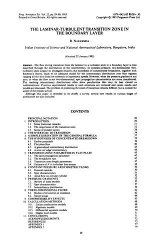
  • 4. 32 R. Narasimha U Reynolds (1883) LEADING Emmons(1951) TURBULENT ~EDGE ~ ~ SPOT ~ ~ ~ TURBULENT Fro. 1. Development of the 'island of turbulence' idea, from the one-dimensional 'flashes' of Reynolds (1883) to the two-dimensional 'spots' of Emmons (1951). The key variable during transition is the 'intermittency', which may be defined as the fraction of time that the flow is turbulent at any point. Now although the Schubauer-Klebanoff experiments provided incontrovertible evidence for the spot concept of transition, the intermittency measurements reported did not agree with Emmons's theory; indeed, Schubauer and Klebanoff fitted their data to an error function curve which had no obvious connection with that theory. This paradox was resolved by the hypothesis of concentrated breakdown (Narasimha, 1957), which successfully explained the observed distribution by proposing a radically different assignment of the a priori probability of spot formation. Dhawan and Narasimha (1958) then showed that with this hypothesis all mean flow properties in a flat plate boundary layer could be predicted very well in what we shall call the transition zone--namely the region of flow that begins with the appearance of turbulent spots and ends through an asymptotic approach to the fully turbulent flow far downstream. 1.2. THE IMPORTANCE OF THE TRANSITION ZONE Let us take a quick look at a few applications where the transition zone plays an important role. Figure 2, based on a study reported by Turner (1971), shows the heat transfer coefficient on the two sides of an internally cooled turbine blade, at different free- stream turbulence levels. Note that there are extensive regions of favourable pressure gradient on both surfaces. The peak heat transfer rate, which occurs on the convex surface, is appreciably higher than would be expected if the flow were turbulent from the leading edge, as can be seen by comparison with the results calculated by the methods of Spalding and Patankar (1967). It is now well known that such peaks (which have long been known in surface skin friction coefficient as well, see, e.g. Coles, 1954), are associated with transition, and tend to occur towards the end of the transition zone. Note also how the onset of transition is unaffected by turbulence level up to 2.2 ~o, but has moved rapidly forward at 5.9 ~o. On the concave surface, on the other hand, the effects are not so clear- cut, but at the highest turbulence levels transition appears to occur early. These observations show how heat transfer rates are strongly influenced by complex interactions between free-stream disturbances, surface pressure distribution and curvature and transition location. A second example is provided by Masaki and Yakura's (1969) interesting analysis of heat transfer on lifting re-entry vehicles such as the Space Shuttle. The design of the thermal protection system, which could account for more than 10 ~o of the empty weight on such vehicles, is crucially affected by the peak heat transfer rate, which is determined by the flow in the transition zone. Masaki and Yakura point out that a drop in the design peak temperature of about 500° F ('-~280° C), which may well be justified by more accurate
  • 5. Laminar-turbulent transition zone localvelocity o exit velocity 1.0 ~ ~ o ~o IconCavesurfacel ~ convexsurfacel I h 200 0 I00 w.-- laminar, flat plate E-- turbulent,flat plate .... turbulent,Spalding- Potankarmethod I I I00 50 ~ stagnation point circularcylinder I I 0 50% chord 33 FIG.2. Heat transfer rate on a turbineblade(basedon Turner, 1971~Top, blade section.Middle,external velocity distribution on blade surface Bottom, local heat transfer coefficient(in units of CHU/ft2h °C:multiply by 1.753 to convert to W/m2K)along chord at different free-streamturbulence levelsq, at an exit Mach number of 0.75. Note that at q= 5.9,about 80% of the convexsurfaceof the blade is in the transition zone. and realistic transition zone models than the 'instantaneous transition' type we mentioned above, may be sufficient to allow changes in the design concept of the protection system. Figure 3 illustrates the large changes in estimated peak temperature depending on the assumed onset and zone-length Reynolds numbers. Indeed, considerations concerning temperature 2OO0 =C q IOeReb=0.75 -IkO~/Om z I 2 3 Ree/Reb 4 FIG.3. Effectof transition zoneparameterson the peakradiation equilibrium temperatureon a typical lifting re- entry vehicle(Masaki and Yakura, 1969).Reb is onset Reynoldsnumber and Ree/Reb is end-to-onsetReynolds numberratio. JP&S 22:1-C
  • 6. 34 R. Narasimha transition play a major role in the design of optimum configurations for re-entry vehicles (e.g. Linet al., 1984). With the extraordinary increase in fuel costs that the last decade has seen, energy efficiency has become an important objective in aerospace engineering. This has rekindled interest in such technologies as relaminarization (Narasimha and Sreenivasan, 1979), turbulent drag reduction (Bushnell, 1983) and transition control (Liepmann and Nosenchuck, 1982). Development of these ideas is likely to demand a better understanding of the transition zone, as successful designs utilizing such ideas may well involve extensive areas of transitional flow. 1.3. SCOPE OF PRESENT SURVEY The plan of this article is as follows. The next section provides a brief survey of recent developments in the understanding of the flow processes preceding the onset of transition and the birth of a spot. Section 3 provides a general statistical framework relating the probability of encountering turbulent flow at any streamwise station, i.e. the intermittency ?, to the generation and propagation of turbulent spots. We present here a new derivation of Emmons's basic formula.Section 4 discusses the hypothesis of concentrated breakdown (Narasimha, 1957) and the generalized intermittency distribution resulting from its application. Section 5 considers the constant-pressure boundary layer on the flat plate in detail and presents spot formation rates in terms of a new non-dimensional parameter, leading to better estimates of transition zone lengths. Section 6 extends these results to constant-pressure axisymmetric flow and Section 7 discusses the effects of pressure gradient. Section 8 briefly examines some three-dimensional flows, including swept wings and slender bodies at incidence. Section 9 considers compressibility effects. Section 10 provides a critical survey of various numerical models for the transition zone that are in current use. Section 11 is a concluding summary. 2. THE OVERTURE TO TRANSITION Although this paper is chiefly concerned with the flow that follows breakdown and birth of a spot, it is worthwhile to review briefly the flow processes preceding transition. These are perhaps best viewed as a sequence of instabilities. Although there is no complete agreement on what the various stages are and on the precise order in which they occur, and indeed there may be no unique route to transition, certain 'milestones' on this route can, broadly speaking, be distinguished in a flow that is not subjected to large external disturbances. These milestones mark successively the appearance of: (1) linear two-dimensional Tollmien instability waves; (2) spanwise variations, with the 'peaks' and 'valleys' observed by Klebanoff et al. (1962); (3) intense 'spikes' in the velocity signal especially in the peak regions; (4) chaotic motion in a 'turbulent' spot, characterised by velocity fluctuations in a broad spectral band. There are almost certainly distinct stages between some of these milestones, but their precise sequence and significance are not yet entirely clear, although some very illuminating experimental observations have recently been reported, in particular by Hama, Nishioka and their co-workers. The initial growth of Tollmien waves is now well-understood, and is adequately predicted by linear stability theory. As wave amplitudes grow it is found that a spanwise variation in flow quantities eventually develops. This spanwise structure was studied in detail by Klebanoff et al. (1962), who triggered it by attaching strips of tape at equal intervals across the plate. Measurements revealed the appearance of counter-rotating vortices, and the development of definite 'peaks' and 'valleys' in the longitudinal fluctuation intensity t~= (/,/,2)1/2. As the spanwise variation intensifies, a thin, high-shear
  • 7. Laminar-turbulent transition zone 35 layer appears, especially at the peak, as observed by Kovasznay et al. (1962). Stuart (1965) has shown that, in a flow with longitudinal vorticity periodic in the spanwise direction, convection and vortex-stretching produce small, intense shear layers resembling those observed experimentally. Such a layer, possessing an inflexion point, is inviscid-unstable, and can lead to further high frequency modes, with the appearance of what have been called 'spikes' in the velocity signal. The flow processes beginning with the appearance of peaks and valleys and leading to spikes have been the subject of much controversy. Klebanoff et al. concluded from their work that these processes were broadly in accord with the Benney-Lin (1960) theory. This theory predicts the emergence of a counter-rotating pair of vortices, for which there is indeed experimental evidence. However, the prediction of the location of these vortices, and of the presence of a second pair below the critical layer, are not in accord with observations. Williams et al. (1984) have recently made a detailed study in a water channel in which they have been able to measure all three components of the vorticity using constant temperature hot film anemometry. These measurements clearly show the presence of two structures: (1) a vortex loop in the flow, of the kind observed much earlier by Hama and Nutant (1963), and (2) a high-shear layer, above the loop and slightly behind its tip. The largest instantaneous vorticity does not reside in the loop but in the high-shear layer above and is predominantly spanwise. There is, in fact, an additional region of strong vorticity, between the vortex loop and the fiat plate; here the vorticity is both longitudinal and spanwise and is spread over a thin, nearly horizontal layer. Williams et al. argue that there is a coherent lump of fluid between the legs of the loop and travelling with it, and that the high-shear layer results from faster flow past the loop above it. Furthermore, the vortex loop, according to them, is the result of the three- dimensional distortion suffered by the coherent fluid within the cat's-eye pattern near the critical layer of the Tollmien theory. It may be noted that, although this region has closed streamlines in a frame riding with the Tollmien wave, the vorticity residing therein is not high, explaining why the vortex loop is not much stronger. Wortmann's (1981) hydrogen bubble pictures also support the vortex loop concept. Calculations by Fasel (1980) show how the vortex loop develops from the vorticity in the 'cat's eye' of the Tollmien wave. These studies indicate that the spike observed by Klebanoff et al. signals the passage of the top of the vortex loop. Concurrently, there have been some interesting developments in the theory of secondary instability. In plane Poiseauille flow, Orszag and Patera (1982, 1983) and Herbert (1983, 1984) have presented calculations viewing the onset of three-dimensionality as a parametric instability problem of a flow carrying finite-amplitude Tollmien-Schlichting waves. This is a linear analysis that leads to Hill- or Mathieu-type equations, and indicates instability in a broad band of spanwise wavelengths. (It may be useful to note an analogy with the non-linear vibration of stretched strings (Narasimha, 1971). In forced oscillations just beyond the natural frequency, the string always goes into whirling motion even if the forcing is strictly plane. The onset of whirling---or three-dimensionality in the motion--is triggered by a secondary instability of the string oscillating in a plane, and can be understood by an analysis of the Mathieu-type.) Herbert shows that such a secondary instability can amplify much faster than the primary (Tollmien-Schlichting) type. The variation in amplitude of both primary and sub-harmonic modes predicted by theory is in good agreement with the measurements of Kachanov and Levchenko (1982, 1984) and Saric and Thomas (1983). The appearance and growth of spikes have been investigated in particular by Nishioka and co-workers (1980, 1981, 1983) in a two-dimensional channel. The flow here was excited by a vibrating ribbon and measurements were made at a fixed station about 24 channel heights downstream, as ribbon amplitude was increased, using a single hotwire probe sensing the longitudinal velocity fluctuation. It was found that the flow rapidly went through various stages involving five or more spikes in a periodic pattern. One of the most interesting findings was that, at this stage, there was already considerable resemblance with fully turbulent flow--the conditionally averaged velocity distribution exhibited a log
  • 8. 36 R. Narasimha law region, spanwise scales near the wall were approximately 80 wall units, and ensemble- averaged velocity signals showed, e.g. strong acceleration phases as in fully turbulent flow. Nishioka et al. (1981) say: "Could this then be called the beginning of a turbulent spot? We do not know." Most of the experiments we have mentioned so far unfortunately do not continue measurement all the way into the transition zone. The exception is the work of Arnal et al. (1977), who studied transition in axial flow along a cylinder of 60 mm diameter and 1200 mm length. Narasimha (1984a) has analysed these experiments and shown that transition on this body must have been largely two-dimensional; he has also determined the effective location of the onset of transition x, from the intermittency measurements in the transition zone, using the methods and conclusions that we shall discuss below in Section 4. His summary of the sequence of 'milestone events' during transition is reproduced in Fig. 4 and leads to the following important conclusions: (1) the location of the onset of transition xt, as determined through intermittency plots by the method of Narasimha (1957), is very close to the station where double spikes appear; (2) the effective length of the transition zone, say between xt and 99 ~o intermittency, is about 0.5 m, which is at least ten times larger than the region covering the distance between the first appearance of spikes (x > 0.705 m) and of spots (x ~- 0.75 m)--this region being at most 0.05 m long. This analysis, taken together with Herbert's recent work, suggests that the complex of problems associated with transition can be largely covered by linear stability theories and transition-zone statistical models; this leaves only a small region just upstream of where spots are born requiring nonlinear stability considerations. When the disturbances are not very low, it is likely that the spanwise periodicity of the peaks and valleys mentioned above will not be so clear-cut; indeed, even the two- dimensional Tollmien waves may be 'by-passed' (to use Morkovin's phrase). Gaster (1975, 1978) has shown how a point disturbance evolves, in linear theory for a growing layer, into a three-dimensional wave-packet because of the dispersion of the instability waves. This flow _ _ stagnationpoint 0 ~'~ ~onset of Tollmien- Schlichtinginstability, in Blasiusboundary layer~ m ~ 0.5 - ,.~ T-S waves on low frequencycarrier ~ ///laminar flow, no spikes lion of transition onset ~T~ "'-"end of laminarregime"',double spikes; ~,',~ occasional spots '~,"'-y" =o. z5 ' °" ~'7" =0.55 ,.o_ m ._ ~~,~ ~, =0.85 ,2-,~last measurementstation -~end of body T x), =0.95 (estimateby extropoltion)~ ~estimates from Narasimha (1984), other events from Arnal et al. (1977]. FIG. 4. Events during transition from laminar to turbulent flow, from the experiments of Arnal et al. (1977). The estimated location for onset of instability does not take into account the favourable pressure gradient that must prevail over the nose of the body, as this gradient is not reported.
  • 9. Laminar-turbulenttransitionzone 37 wave-packet is of course not a turbulent spot by any means, but it is possible that its structure has features that may be relevant to understanding the spot. To conclude this section, we may remark that recent observations and theoretical developments have helped to shed much light on the later stages of instability before the onset of transition. These may help us eventually in predictin# the onset of transition, but that still seems not likely in the very near future. Some years ago Reshotko (1976) wrote, "These efforts, however, have yielded neither an acceptable transition theory nor any even moderately reliable means of predicting transition." This still seems largely true; we shall touch on the problem briefly in an Appendix. Meanwhile, as we have just pointed out, the extent of the transition zone is generally comparable to the extent of laminar flow, and far longer than the region in which strong nonlinear effects control flow development. Thus, to appreciate the entire structure of the flow, and to calculate it in technological applications, it is necessary to devote greater attention to the transition zone itself, i.e. to the flow following onset, than it has generally received. It is the purpose of this article to restore the balance. 3. A SIMPLE DERIVATION OF THE GENERAL FORMULA Consider the flow past a surface on which is embedded a coordinate system xy (not necessarily Cartesian, see Fig. 5). The coordinate z is normal to the surface. We consider the intermittency as a function of (x,y) only, ~ = ~,(x,y); ~ does vary with z, as shown by Dhawan and Narasimha (1958), but this variation is akin to the outer or 'edge' FIG.5.Thecoordinatesystem. intermittency of any (fully) turbulent boundary layer, which we shall discuss briefly in Section 4; the intermittency significant for transition is the value at the surface z = 0, and we may think of 7(x,y) as this value. (Although the velocity is zero at the surface, and so cannot be intermittent, the velocity gradient or wall stress can be. Indeed, ~(x~v)is perhaps best measured using surface instrumentation such as hot film gauges, as Owen (1970) has done.) Following Emmons (1951), consider now xyt space, where t is time. A spot generated at a point Po(xoYoto)will, in general, sweep out a volume in xyt space, called the propagation cone; a section along t = const, gives the planform of the spot on the body surface at time t (Fig. 6). We can define further a 'dependence' cone for Po as the set of all points in xyt space such that spots generated at those points will cover Po (also illustrated in Fig. 6). If the flow is stationary in time, a translation in time will just shift both cones up and down for given (XoYo).If the spots propagate with constant velocity, the cones will have straight generators, and all parallel sections of the cones will be similar. In postulating the existence of such cones, we have supposed that they are uniquely determined at each point. We may more explicitly state the following 'independence hypothesis': the presence of a spot anywhere in the flow does not affect the generation or propagation of other spots at other points in the flow. (3.1)
  • 10. 38 R. Narasimha I oo ~/'I",~ L~,-, ) cone R FIG. 6. Propagation and dependence regions for any point on a surface in the flow. This implies, in particular, that when two or more spots intersect on xy, the area covered by them at any instant is just the union of the areas that would have been covered by each spot individually at that instant; velocities are unaffected. This was shown to be true for two spots by Elder (1960), but the hypothesis (3.1) is unlikely to be strictly valid in more general situations. Indeed, the work of Coles and Savas (1980) suggests that spots generated very close to each other do affect their propagation. (However, this conclusion is based on hot wire measurements midway across the boundary layer, where edge intermittency is already significant; it is important to see if surface gauges show a similar effect. Also the regular hexagonal array on which spot production was forced in these experiments may have been responsible for some of the observed effects.) Wygnanski et al. (1979) have shown that once a spot is generated, it induces a flow in the neighbourhood that may trigger other spots. Nevertheless, if the spots are spaced sufficiently far from each other, an 'independence' hypothesis like (3.1) may be a reasonable approximation. We now further assume that, if dS(x,y) is an element of area on the surface: there is a function 9(x,y,t) such that the probability that a spot is formed in the volume element d V = dS(x,y,)dt is 9 d V + o(d V). (3.2) This is similar to the 'orderliness' assumption introduced by Khintchine (1960) in his discussion of queues, and implies that the probability that two or more spots will be born near the same place around the same time is relatively small. It can then be easily shown that the mean number of spots generated in dV is also 9 dV, so that 9 is also a turbulent source-rate density. The two hypotheses we have made imply that spot production is a Poisson process. In fact, beyond this point there is a close analogy with the theory of queues. The statistics of spots is related, e.g. to that of telephone traffic, and that of intermittency to the corresponding busy times, except that a generalization of classical queueing theory (with just time as the single independent variable) is required to handle the three-dimensional xyt space. Thus, with a straightforward extension of Khintchine's arguments, we can show by any of a variety of methods that the probability that no source occurs in a finite volume V is just exp - S g(x', y', t') dV'. (3.3) V (The analogue in the telephone queue is the probability that there is no call during a given finite time interval.) Further, as the flow at P is turbulent only if there is at least one spot in the dependence cone (say R(P)) for P, it follows that the probability of turbulent flow at P is just the complement of Eq. (3.3), i.e.
  • 11. Laminar-turbulenttransitionzone 39 ~(P) = 7 (x,y,t) = 1-exp r- Sg(x',y',t') dV']. (3.4) n(P) This is the general formula given by Emmons in 1951. To derive it he had to formulate and solve an integral equation, and limit himself to a flat surface (a simpler derivation was given by Steketee in 1955). The present demonstration of the result amounts to recognizing that we can postulate the spot formation process to be a nonstationary Poisson stream in xyt space, obeying Khintchine's hypotheses of 'absence of after-effects' (or independence) and 'orderliness'. We may note that although the result (Eq. (3.4)) is valid even when g(x,y,t) is 'nonstationary' in all variables, we will generally assume stationarity in t (so that g is time- independent) but not necessarily in x, y. It may finally be remarked that while the assumptions (Eqs (3.1) and (3.2)) are sufficient to yield Eq. (3.4), they are not necessary; Eq. (3.4) would be valid under weaker conditions. For example, the 'eddy transposition' observed by Coles and Savas (1980) would invalidate part of Eq. (3.1), but would not affect the intermittency (Eq. (3.4)) if the transposition were to leave unaffected the magnitude of the area covered by turbulence at any station. Experience with application (as we shall see below) indicates that even if Eq. (3.1) may not be literally correct under certain extreme conditions, Eq. (3.4) provides an effective tool for understanding observed intermittency distributions. 4. THE HYPOTHESIS OF CONCENTRATED BREAKDOWN 4.1. EARLIERPROPOSALS To derive an intermittency distribution it remains to determine, or guess, the form of the function g. Let us now restrict attention, for the moment, to constant pressure flow past a fiat plate. When the flow is two-dimensional and steady, g can depend only on x, g = g(x). One possible assumption here--the one picked as natural by Emmons--was to take g = const., independent even of x (Fig. 1), i.e. it was considered that the probability that a spot would be born was the same everywhere on the plate. (Later Emmons and Bryson (1952) considered g(x) = ( ) x", n > 1, arguing that g may increase with x as the flow becomes increasingly unstable downstream with increasing Reynolds number.) If it is further assumed that the spot propagates linearly in both space and time, i.e. that the envelope of spot positions on the surface is a wedge of constant angle and spot propagation velocity is constant at each point on it--then the propagation and dependence cones both have straight generators, and the volume V of the dependence cone for x is proportional to x 3. We can, therefore, write S g d V = g V = (ga/3 U) x3, (4.l) where a is clearly a non-dimensional spot propagation parameter, equal to the base area of the cone at unit distance from the apex. Putting this in Eq. (3.4) immediately leads to the intermittency distribution ~,(x)= 1- exp( - trgx3/3 U). (4.2) Measurements of y quickly show that there are certain features of Eq. (4.2) that cannot even be qualitatively right. First of all, Eq. (4.2) possesses the similarity property that, if .¥ were the point at which y = 1/2, 7 = 1- exp( -(x3/~ 3) In 2), (4.2a) i.e. all intermittency distributions should collapse when plotted vs. x/~. This just does not happen, as Fig. 7 demonstrates. (Here, and in the rest of the paper, we shall identify the flows studied by the code adopted by Dey and Narasimha (1983), an extract from which appears in Table 1.)
  • 12. 40 R. Narasimha X 1.0 0.5- 0 0 ,958) /.j Nzo2 Cf 0.5 1.0 1.5 x /7 FIG. 7. Intermittency data from two experiments (Narasimha, 1958) showing no similarity in distribution with the variable x/.~, where .~ is the location of y= 0.5. TABLE 1. LISTOF FLOWSCITED Reference Code Agent Remarks Abu-Ghannam and Shaw (1980) ASZI -- Narasimha et al. (1984a) Narasimha (1958) Narasimha (1958} Rao (1974) Schubauer and Klebanoff (1955) ASFI ASAI DFU3 1/16 in. grid DAUI 1/16 in. grid NFUI wake of rod NFDI wake of rod NZ01 NZ02 wake of rod NZ03 wake of rod NZ04 wake of rod NZ05 1/2 in. grid NZ06 wire trip NZ07 wire trip RCL2 grid SKZI -- SKZ3 wire trip SKZ4 grid Read from Fig. 14 of reference; fixed tunnel speed of 20 m/s, zero pressure gradient Favourable pressure gradient; same source Adverse pressure gradient; same source Favourable pressure gradient in upstream part of transition zone; U = 12.0 m/s Generally adverse gradient, but slight favourable gradient near onset; U= 13.4 m/s Favourable pressure gradient in upstream part of transition zone Favourable pressure gradient in downstream part of transition zone 'Natural' transition; U=54 ft/s, Re~= 1.06 x 10⁶ U=54 ft/s, Re,=0.3 x 10⁶ U=54 ft/s, Ret=0.05 x 10⁶ U=49 ft/s, Ret=0.44 × 10⁶ U=43 ft/s, Ret=0.36 x 10⁶ U= 54 ft/s, Rez=0.19 × 10⁶ U=46 ft/s, Re~=0.29 × 10⁶ RG= 6,450, d= 3/4", L region U=80 ft/s, Re~=2/31 x 106 U = 30 ft/s U=35 ft/s Secondly, if any mean flow parameter, like the skin friction coefficient, for example, was computed at any station x using 7 by mixing the laminar and turbulent values cy~, cy, (corresponding to that station) in proportion, Cf : (1 - 7) Cfl "~ Cft, (4.3) the distribution of cI so computed using Eq. (4.2) for 7 shows a smooth variation from the laminar to the turbulent value, the latter being always approached from below. However, measurements show that cy actually overshoots the turbulent value during transition; so does the surface heat transfer coefficient in high speed flows (as the experimental data shown in Fig. lb already demonstrate)--which is one reason why accurate modelling of the transition zone is important. 4.2. FLAT PLATE FLOW A simple explanation for the overshoot in skin friction and heat flux during transition is that the virtual origin of the turbulent boundary layer, which develops after transition, is not at the leading edge of the plate but at some station further downstream. Based on
  • 13. Laminar-turbulent transition zone 41 ,, s.ot / ,:,< , 1 g t FI(3.8. Picture of transition with concentrated breakdown as suggestedby Narasimha (1957).Spots are born with equal probability along the linex=xt, but not upstream or downstream: compare Fig. la. considerations like this, and an analysis of measured intermittency distributions,* Narasimha (1957) proposed a different assignment of equal a priori probabilities in the form of the hypothesis of 'local' or 'concentrated' breakdown, which can be stated as follows (see Fig. 8): spots form at a preferred streamwise location randomly in time and in cross-stream position. (4.4) This appeared consistent with the observation of Schubauer and Klebanoff (1955) that no breakdowns occurred on the plate before a certain point was reached or much further downstream. This point may be identified with the beginning or onset of transition, x,. An appropriate idealization then was to take 9 as a Dirac delta function, O(x) = nf(x - x,), (4.5) where n is the number of breakdowns or spots occurring per unit time and spanwise distance at Xr The corresponding intermittency distribution is If we use the distance y = 1 - exp[ - (x -x,)2na/U] (x >_x,), = 0 (x <x,). (4.6) 2 = x(y = 0.75)-x(y = 0.25) (4.7) to characterize the extent of the transition zone, Eq. (4.6) becomes the 'universal' distribution (Narasimha, 1957) y = 1-exp[-0.412 ~z], ¢ = = (x-x,)~2. (4.8) Narasimha showed that his own measurements, and those of Schubauer and Klebanoff, agreed very well with Eq. (4.8). Perhaps the most striking evidence from more recent measurement* comes from Owen (1970), who used surface hot film gauges to measure (Fig. 9). Of course Eq. (4.5) cannot be literally correct; all that can be said is that the breakdowns occur effectively in a belt across the flow whose width is small compared with the extent of *Assumingthat the dependence cone has straight generators, Narasimha (1957)showed that g(x) = - (U/2a) (da/dxa) In (1- 7), so that g(x) can, in principle,be obtained from measured7. In practice,the required numerical differentiation of experimental data is hard to perform, but does suggest the hypothesis (4.4),as In(1-),) turns out to be nearly parabolic with vertex at a fairly well-definedpoint x, implying that g = 0 everywhereelse. tQuestions concerning how to measure 7 unambiguously from probe outputs are not trivial, and are briefly considered in Appendix 1.
  • 14. 42 R. Narasimha y I00 - % 80- 60- 40 20 0 i / h.oryN ° r O . i m h I o9::i experimentol I • 4.8 x IOs data (Owen 1970)1 • 6.4xt0 s i I I I 0 I 2 3 { FIG. 9. Intermittency distribution during transition on a fiat plate measured using hot film gauges, compared with theory (Owen, 1970). the transitional region. By examining the results presented by Dhawan and Narasimha (1958) for Gaussian distributions of g, one can estimate the width of this belt to be no more than about a third of 2, and very likely rather less. If 7 is measured, x, is best obtained by plotting the function F(y) = = [ - ln(l - y)] 1/2, (4.9) introduced by Narasimha (1957), against x and extrapolating to F = 0 from the best fit of a straight line to the plot (see Fig. I0). This procedure is desirable both because Eq. (4.6) may y 0.99 0.98 O.S5 09 0.5 expt. o SKZI ~. SKZ3 o SKZ 4 • NZOI o NZ02 o NZ03 o NZ04 • NZ05 o NZ05 • NZ06 v NZ07 0 L.O r i , , i I i • • o o 0 ~ o I 2.10 3.0 FIG. 10. The F(~) plot, showing linearity in x and the universality of the intermittency distribution in the transition zone of a constant pressure boundary layer, with a variety of agents for forcing transition. Compare Fig. 7 (Narasimha, 1957). not be accurate near x = x, and because the small values of ~,near xt are hard to measure accurately and so are subject to some error.* It may turn out that at x, so determined, an occasional turbulent patch would be observed, nevertheless this xt is the most appropriate definition for the onset of transition, if only because it happens also to be the effective origin of the fully turbulent boundary layer at the end of transition. Dhawan and Narasimha (1958) showed that all mean flow parameters during transition could be very satisfactorily explained using the distribution of Eq. (4.8), mixing a laminar boundary layer from the leading edge with a turbulent boundary layer originating at x, in the proportion 1-7 to ~,. (This assumes that the ensemble average of the spots over time and span is the usual two-dimensional turbulent boundary layer beginning at Xr I do not *For two reasons: (1) to get an adequate number of turbulent patches requires a long record and (2) result for 7 depends sensitively on discrimination procedure adopted (see Narasimha et aL 1984a).
  • 15. Laminar-turbulent transition zone 43 know of a direct verification of this assumption yet, although a variety of other but similar ensemble averages have been measured for spots in recent years, in particular by Arnal et aL, 1977). In particular, the overshoot in skin friction that was mentioned earlier, and a dip in the displacement thickness just after onset often noticed in experiments (Fig, 11), are both well-predicted. The former is a simple consequence of the origin of the final turbulent boundary layer being at xt and not at the leading edge of the plate. The latter has the simple physical explanation that where the thicknesses of the (alternating) laminar and turbulent boundary layers are comparable, a combination of the above kind must lead to a reduction in 6" from the laminar value, as the turbulent profile is fuller; this again would not happen if the turbulent boundary layer originated at x = 0. 0.04 ft | ~ / o experiment, SKZ I 0 ~" 0 0.004- ft. ~#," ,~s 7, 0 --" "" ~" 0 I I o l 2 ~ ¢ -0~, Fro. 11. The variation of boundary layer thicknesses during transition: experiment compared with theory (Dhawan and Narasimha, 1958). Note how well the observed dip in 6* is predicted. The distribution of Eq. (4.6) has been found useful in a variety of flow situations, including, e.g. swept wings (Poll, 1978) and hypersonic speeds (Owen and Horstman, 1972); it has also formed the basis for several transition zone models (e.g. Adams, 1970; Harris, 1971). However, there are also situations, involving strong pressure gradients or cylinder- like geometries, where modifications are needed (Narasimha, 1984b). We shall discuss these issues in subsequent sections. The hypothesis (4.4) thus seems to provide a satisfactory resolution between the conflicting pictures of a 'sudden' transition (Dryden, 1939) and a 'gradual' variation (Prandtl, 1935) of boundary layer parameters through the transition zone. 4.3. A GENERALIZED INTERMITTENCY DISTRIBUTION Consider now arbitrary three-dimensional flows. If we accept the hypothesis of concentrated breakdown, only the intersection (say Rt(P)) of the dependence cone R with the surface x = x, is relevant for determining y at P. The probability that at least one spot occurs in Rt is then just exp- S ndA,(P) where n is the number of breakdowns per unit area of Rt and At is the area of R,; we thus obtain (Narasimha, 1984b) 7(P) = 1- exp - SndAt(P). (4.10) If we assume that spot formation is stationary in time and homogeneous across x, Eq. (4.10) simplifies to 7(P) = 1- exp[ - nAt(P)]; (4.11)
  • 16. 44 R. Narasimha the problem of finding the form of the intermittency distribution is therefore reduced to that of finding At(P), which we may appropriately call the 'dependence area for P'. Furthermore, from Eq. (4.9), F 2 = nAt(P), (4.12) showing that the function F of Eq. (4.9) is just proportional to the square root of the dependence area. We shall encounter applications of Eqs (4.11) and (4.12) in Section 6. 4.4. A NOTE ON 'EDGE' INTERMITTENCY Before moving on to a discussion of other consequences of Eq. (4.6), it is worth pointing out that the transitional intermittency we are discussing should be distinguished from the 'edge' intermittency characterising the outer fluctuating boundary (albeit highly convoluted) of even fully turbulent flows. (There is even a third kind, which may be called 'small eddy' intermittency, associated with the spottiness of dissipating eddies and revealed as pulses of activity when turbulent signals are filtered at high frequencies, but this will not concern us here.) A transitional boundary layer possesses an edge intermittency as well, whose variation with height has been discussed by Dhawan and Narasimha (1958) and Owen (1970). There does not appear to be any direct connection between these intermittencies. However, Maeda (1968) has made the interesting proposal that the edge intermittency 7e of the turbulent boundary layer can also be described in terms of the transitional distribution (Eq. (4.8)). He puts 7e(z) = exp[-O.412(Z-Zo)2/22] {z>--Zo} where 2, is a measure of the spread defined exactly as in Eq. (4.7). Experiment shows excellent agreement with this distribution (Fig. 12). I feel that this agreement is perhaps I-),e 1.0 0.8- 0.6- O.4- 0.2- I I l I I I 0 O.5 I.O [.5 2.0 2.5 3.0 ~¢ FIG. 12. Edge interminency in boundary layer, fitted to the universal intermittency distribution (Eq. (4.8)) (Maeda, 1968). best explained by imagining laminar patches emanating in a Poisson stream from the edge of an inner (full-time turbulent) layer; from Fig. 23 of Maeda's paper, this edge z0 appears to be nearly at the end of the log region in the velocity profile. It is then easy to see from the general argument of Section 3 that the variation of the probability of non-turbulent flow with height above the surface obeys the same law as the streamwise variation of the probability of turbulent flow during transition. Of course, similar assumptions need to be made in both cases to derive the distribution, but we may note that the idea that large eddies pass any flow station in a Poisson stream is independently supported by the zero- crossing data of Sreenivasan et al. (1983).
  • 17. Laminar-turbulenttransition zone 5. TRANSrrloN ZONE PARAMETERS IN FLAT PLATE 45 The distribution (4.6) has three unknowns: xt, 2 and n. The numerous and extraordinary problems associated with the prediction of the onset of transition for engineering applications, or even of analysing experimental data, have been discussed at length by Morkovin (1969, 1971, 1977) and Reshotko (1976). To these may be added the collection of papers on "Recent developments in boundary-layer transition research" that appeared in the AIAA Journal of March 1975. All these studies emphasize determination of transition onset at high speeds. The present paper, on the other hand, is more concerned with the flow following onset; we shall therefore content ourselves with a brief discussion of the onset-prediction problem in Appendix 2. We now present estimates of a and n in constant pressure flow, although for prediction of ~ it suffices to know the product nor. 5.1. THE SPOT PROPAGATIONPARAMETER By comparing Eqs (4.6) and (4.11) we have in a constant pressure two-dimensional boundary layer A, = a(x - xt)2/U. (5.1) a here is the spot propagation parameter (perhaps better called the dependence area factor from the present point of view) defined by Emmons (1951), and can be written as (Narasimha, 1978) a = Ut I [b(x,t)dx]/x3 (5.2) where b is the width of a spot generated at t = 0, x = 0 and the integration is carried out over the spot at time t. Emmons estimated the value of a as about 0.1, based on indirect evidence. Narasimha (1978) has performed the integration in Eq. (5.2) based on the experimental data of Schubauer and Klebanoff (1955), and found that tr varies from about 0.25 for the spot shape given by them close to the wall, to about 0.29 for the second shape somewhat away from it; far away from the wall a must, of course, fall to zero. Spot spread rates vary slowly with the Reynolds number (e.g. Narasimha et al., 1984b), so we may expect, to do the same, but there is not enough data to provide quantitative estimates. 5.2. THE BREAKDOWNRATE Putting Eq. (4.7) into the intermittency distribution (Eq. (4.6)), it is easy to show that n = 0.412 U/a 22; (5.3) equivalently (taking the opportunity to correct a 25-year old misprint on Fig. 5 of Dhawan and Narasimha, 1958), Re~ = 0.642 r~-1/2, r~= = ntr v2/U 3 (5.4) being a non-dimensional spot formation rate. The extent of the transition zone, therefore, varies as the inverse square root of the breakdown rate and information on Re~ provides estimates of n. Dhawan and Narasimha (1958) sought to find out whether there was a well-defined relationship between Re~ and Re r Their examination of available data showed considerable scatter (see Fig. 13), partly because there are widely differing definitions of the beginning and end of the transition zone, and partly because data at various Mach numbers, disturbance levels, etc. are all included. Nevertheless, the data do indicate that Re~ increases with Ret but not as rapidly; in fact, Dhawan and Narasimha suggested the rough correlation Re~ - 5 R°'a. (5.5)
  • 18. 46 R. Narasimha ,,,Re X" ,o6 present proposal, 9 Ret5/4 I i05 .El"/ 5y ~si ," ,5 Ret0"8 '1106 r i Ret FzG. 13. Relation between onset Reynolds number Re r and the extent of the transition zone as measured by the Reynolds number Re (data from Dhawan and Narasimha, 1958). If the exponent here had been unity, then ~-distributions would have shown similarity in x/.¥ as in Eq. (4.2a); ;t would then have been proportional to .¥ or xt and there would have been only one length scale in the problem. As we have already seen in Fig. 7, however, this is not the case. In spite of the scatter of the data points in Fig. 13, the correlation (Eq. (5.5)) has been found effective in many recent studies (e.g. Abu-Ghannam and Shaw 1980; Gostelow and Ramachandran, 1983). It was, however, noted by Narasimha (1978) that a change in exponent from 0.8 to 0.75 in Eq. (5.5) would still be consistent with the Dhawan-Narasimha data, and would lead to the significant conclusion that n depends primarily on the local boundary layer thickness. In Fig. 13 is also shown the proposed new correlation Re~ ~- 9 Re3t/4, (5.6) along with Eq. (5.5) and the data. It is easy to show from Eqs (5.6) and (5.3) (see also Narasimha, 1984b) that the appropriate non-dimensional parameter for the breakdown rate is naO~/v(which we shall briefly call the 'crumble'). As we shall see in the next section it has the approximate value N = (naO3)/v ---0.7 x 10⁻³, (5.7) where 0t is the momentum thickness at xf. If we took the Blasius boundary layer thickness at xt as fit---5xt Re~~/2, Eq. (5.7) becomes rl(~t3/V~---2. (5.8) This clearly suggests that the breakdown rate scales primarily with the boundary layer thickness and the viscous diffusion time fit2/v--a physically appealing conclusion. In contrast, the parameter ~ was estimated by Dhawan and Narasimha (1958) to vary (depending on Ret) in the range I0 ~1 to I0 ~5 suggesting that U and v are inappropriate scales for n, although they have the convenience of being free-stream parameters. We may expect that, as the hypothesis of concentrated breakdown seems valid independent of disturbance level, pressure gradient or Mach number (as we shall see later), the parameter that will be affected in all these cases will primarily be N.
  • 19. Laminar-turbulent transition zone 47 Using the above relations, the spot formation rate is shown as a function of flow velocity in Fig. 14, for different values of Ret and for air and water (Narasimha, 1978). Note how rapidly n increases with U, and how small n is in water; at 1 m/s and Ret= 3 x 10⁶, there are only a few spots born per second-metre. Surely (to reiterate the conclusion that motivated the calculation) active control of transition here should be possible! IOg (smf' flow velocitywater I IO IOz mls I I v = I0-e m21s for water 15 xlO"e m21s for air Ret =0.3 x I0-'-~-. 1.0 X IOe---~ 30 x IOS----~ 103 - i i i 9 i) I I0 I0 m/s IC~ flow velocity,air FIG. 14. Spot formation rates in air and water flow past flat plates at different onset Reynolds numbers (Narasimha, 1978). 5.3. TRANSmONZONELENGTHPARAMETERS Analysis and interpretation of the numerous experimental investigations that have been conducted by different workers on the transition zone is rendered difficult by the plethora of techniques used for detecting transition and of definitions adopted for identifying the beginning and end of the transition zone. However, Dey and Narasimha (1984a) have recently made a critical analysis of the data and have, in particular, attempted to find relations between the different definitions. Consider, for example, the simple and widely used surface pitot method, in which the beginning and end of transition are identified with the locations of the minimum and maximum, say Xmi,and x m,xrespectively, of the pitot reading. Based on the simultaneous measurements of Narasimha (1958), Dey and Narasimha suggest that in low-speed flow x, ---Xmi,-0.26 (x m~--Xmi,), 2 -'- 0,4 (X~=--Xmi,). (5.9) The same relations seem valid to a good approximation for data using other surface quantities such as wall stress or heat transfer. (However, surface pitot minima are often
  • 20. 48 R,Narasimha not clearly defined at high speeds, where the above relations become either less useful or even invalid (Dey and Narasimha, 1985).) Based on such analysis, tentative equivalences have been established, as shown in Fig. 15. Further verification and refinement are obviously necessary, through studies in which different experimental techniques are used simultaneously. ql fully turbulent ~_~_ flowfrom x~ ; Xmax laminarj" "X-mi n flow -- j x~ - " ~ _ _ ~ . i "~~10.2 52.5X '~~0.2X 0 x t FIG.15, Relationbetweentransitionzoneparametersin incompressibleflow,derivedfromintermittencyand surfacepitotmeasurements(DeyandNarasimha,1984a). 5.4 ESTIMATE OFN IN TURBULENTFREE-STREAM Several interesting and important points first need to be made about the effect of free- stream turbulence on transition. In general, both intensity and scale (and, indeed, the whole spectrum in relation to the transitioning boundary layer) are relevant, but the effect of scale seems weak in experiments designed expressly to reveal them (Hall and Hislop, 1938). This is consistent with Taylor's (1938) analysis, according to which the governing parameter is the number T = q (D/L) 1/5 (5.10) where q is a measure of the turbulence intensity, L is the macroscale and D, a characteristic dimension of the body. The low exponent on L implies that its effect cannot be strong. The success of T in correlating transition data on spheres was demonstrated by Dryden's (1948) classic measurements. The effects of q on transition onset and length are displayed in Figs 16a and b. Here q = 100 (2K/3 U2)1/2,K being the mean value of the turbulent kinetic energy per unit mass. The data from Schubauer and Skramstad (1948) show that Rext generally drops with increasing q, but attains a constant value of about 2.8 x 10⁶ for q < 0.1; this was attributed
  • 21. Laminar-turbulent transition zone 49 0 Re xmin 6- o Wells 1967 v Schubeuer 8 Skromstad 1948 • Brown P, Burton 1977 • Martin etal. 1978 I. m I I l I 0 0.2% 2 4 (a) Orr- Sommerfeld stabilty limit: parallel flow developing flow • - - &, JL. - - - ~ • I l I 6 8% -2R, pmin -4 e•2 0 q (b) onset Reynolds boundary between number ~-IA , IB % -- -- ~ --. ~ / facility-dependent . >~ limits for low turbulence residual turbulence disturbances dominant dominant disturbance - limited .I I rr turbulence intensity FIG. 16. (a) Variation of onset Reynolds number with free-stream turbulence intensity, as measured by various workers. (b) Sketch of the qualitative effect of free-stream turbulence on onset Reynolds number, showing different regimes (Dey and Narasimha, 1984b). Similar regimes can be defined for each disturbance type. by them to the dominance of acoustical disturbances at these low turbulence levels. Wells (1967) finds a similar trend, with Rext levelling off much higher, at about 5.5 x 10⁶, for q < 0.1, but for greater q there is surprisingly good agreement with Schubauer and Skramstad. This clearly shows that no unique value of Re= as q--M) is observed in experiment; the obvious interpretation is that the asymptotic value depends on the residual disturbance level in the tunnel used, and that free-stream turbulence is not the driving agent for transition at low q. Thus, correlations yielding a finite value of Ret as q--4) (e.g. Hall and Gibbings, 1972; Abu-Ghannam and Shaw, 1981) are suspect at low turbulence levels. Figure 16a also shows that at high turbulence levels Ret tends to become independent of q and, in fact, the momentum thickness at onset, Reo, is close to the stability limit (Reo~, = 193 from parallel flow theory, 154 allowing for spatial growth). On this basis, Dey and Narasimha (1984b) propose that three different regimes in q can be distinguished, as sketched in Fig. 16b. At high turbulence level (regime II) transition is stability-limited; the amount of disturbance is not a limiting resource, and the transition Reynolds number is independent of q. Transition at lower q is 'disturbance-limited' (regime I), but at some value of q that would in general depend on the facility, the residual JPAS 22:1-D
  • 22. 50 R. Narasimha non-turbulent disturbances like noise and vibration are responsible for forcing transition (regime IA). There is, therefore, an intermediate range of 'moderate' turbulence, say 0.1 < q<4, where transition is truly turbulence-driven (regime IB). In this regime, Dey and Narasimha (1984b) propose Rext= 0.4 x ]06q 1.2, Rex-'- 10 Ra3/4 -~.~, . (5.11) The values of N may be determined from data on Rea and Rear using the relation N = 0.412 R ,,3/z Re~ -2 ..~, , (5.12) which follows from Eqs (5.4) and (5.7). There are only three data sets, namely Schubauer and Skramstad (1948), Abu-Ghannam and Shaw (1981) and Gostelow and Ramachandran (1983), which permit an estimate of N from Eq. (5.12). The results are shown in Fig. 17. It IOBN o Sehubauer, Skramstad Ig48 <~ Schubauer,Klebanoff1955 o Abu-Ghannarn, Show 1980 A Gostelow, Rarnachandran 1983 o 0 oo n°° o ~, NT=O'7xlO-3 ~ ,~ "~0 o ~ 0 0.1 1.0% q FIG. 17. Variation of non-dimensional spot formation rate with free-stream turbulence level, as inferred by Dey and Narasimha (1984b) from three experimental data sets. The large spread in the Abu-Ghannam-Shaw data is chiefly due to the difficulty of reading from a small diagram. is seen that in each of the data sets shown N drops with increasing q, but tends to approximately the same value of about 0.7 x 10 -3 at high turbulence levels. (The large spread in the Abu-Ghannam-Shaw data is chiefly due to difficulty in reading small differences in an already small diagram.) Considering the difficulty in interpreting the data, and the ignored effect of turbulence scales, it is remarkable that there is such agreement about the value of N. The increase in N at low q may at first appear paradoxical, but it must be remembered that with increasing turbulence 0t drops rapidly, and the actual breakdown rate n therefore goes up. To sum up, we have the important conclusion that: in transition forced by turbulence, the non-dimensional spot formation rate N has the universal value of about 0.7 x 10⁻³. (5.13) 6. CONSTANT PRESSURE AXISYMMETRIC FLOWS 6.1. GENERAL REMARKS We consider here how the ideas of the previous sections can be extended to axisymmetric flows. Data here are not as extensive as on flat plates, and a great deal of work remains to be done, but certain general conclusions can be drawn.
  • 23. Laminar-turbulent transition zone 51 First of all, if the dependence volume is a true cone with straight generators, Af in Eq. (4.11) is proportional to (x -x,) j, wherej is the number of dimensions. For a flat platej = 2; for a pipe or a cylinder with axis aligned to the flow, when the slug fills the pipe or the spot has wrapped itself around the cylinder (we shall discuss this further below), the problem is just one-dimensional, and we get y = 1--exp[--(x--x,)nlG1/U ] (6.1) 7 = 1--exp[- 1.10(x --xt)/2], (6.2) where n is the spot formation rate (number per unit time), and al is a one-dimensional analogue of the dependence area factor of Eq. (5.1), defined by At = a~(x-xt)/U. 2 is still given by Eq. (4.7). The result (Eq. (6.2)) is due to Pantulu (1962), who confirmed it by experiment in pipes (Fig. 18). ), I.O Y =I- exp (-I.I~¢) ~ - : ' ~ 0.8 O.6 v~.,,~ - Re=U.20 Iv /x x 2500 I Rotto 0.2 /" • 2910 Ponlulu / (1962) 0 1 i i I I I 0.5 1.0 1.5 2.0 2.5 5.0 FIG. 18. The one-dimensional universal intermittency law, compared with measurements in pipe (Pantulu, 1962). In the initial stages Of breakdown j = 3 may be relevant; in confined flows permitting no growth, e.g. cylindrical Couette flow (Coles, 1965), j = 0, i.e. ~ remains constant. 6.2. SPOT CHARACTERISTICS Let us briefly consider certain general aspects of the problem. An assumption that is often made in flows with non-parallel streamlines is that the spot propagates across streamlines, the envelope being inclined at a constant angle to the local external streamline everywhere (Emmons and Bryson, 1951; Chen and Thyson, 1971; Rao, 1974). On the nose of an axisymmetric body, this makes the developed envelope a logarithmic spiral; in radial flow past a normal disk, a spot created at a certain point would grow so wide that its edges would eventually come together at an azimuth 180° away from "the point of spot generation. Unfortunately, this hypothesis seems never to have been tested. Work on hand at Bangalore may shed some light on this question. However, what evidence there is does not suggest that anything so spectacular is likely to happen. Thus, the experiments of Braslow et al. (1959), on a 10° cone in supersonic flow, show turbulent wedges of half-angle about the same as in low-speed flow on a flat plate (see Table 2). There is a reduction with wall TABLE2. TURBULENTWEDGEANGLES Reference Spark generator Surface Flow velocity Half-angle Remarks Schubauer-Klebanoff Spark Flat plate Maeh 0 8.5-10.5 Rex~- 106 Narasimha (1958) Roughness element Flat plate Math 0 9 Rex± 2 x 10⁵ Wygnanski (1980) Spark Flat plate Maeh 0 9.3-10 Braslow et al. (1959) Roughness element 10° Math 1.61 11.25 Adiabatic wall 10.5 Cooled wall Math 2.01 8.7 Adiabatic wall 7.5 Cooled wall
  • 24. 52 R. Narasimha cooling and higher Mach number, but nothing to indicate a logarithmic spiral, or any strong departure from a wedge-shaped envelope. Another relevant result here was reported by Gregory (1960) who visualized turbulent wedges on a swept wing. Because of the strong spanwise flow outboard on such a wing, an excrescence placed at the leading edge results in a curved turbulent wedge. Gregory showed (Fig. 19) that the area covered by turbulent flow on the wing could be estimated (lff/C)o. 5 ~x ~at incidence ---B.6 0.6- 0.4- 0.2- 0 excrescence V= 120 ft/s height k(in) a =-5" x 0.025 upper surface zx 0.10 Rec=2.3x10⁶ O~ o 0.25 predicted width, ', /for 6 position of attachment line 0~05 ().10 0'.15 0120 Xk/C J. l 0.f35 l l 0 45 0.40 0.30 x"/c FIG. 19. Turbulent wedges on swept wing (Gregory, 1960). quite well by constructing a wedge of semi-angle 10.6° (a value obtained by Schubauer and Klebanoff (1955) in constant pressure flat plate flow) around the particular streamline at the edge of the boundary layer passing through the excrescence. It would therefore appear that at the present time it is best to: assume that the spot envelope makes a constant angle with the central (rather than the local) external streamline. (6.3) 6.3. AXIAL FLOW ON CIRCULAR CYLINDER Consider now the flow past a circular cylinder of radius a, with axis along the free- stream. From the discussion above, we expect that a spot created at any point on the surface will at first propagate as in plane flow on the developed surface; at a certain station x* the spot will wrap around the cylinder, and propagate like a sleeve thereafter (see Fig. 20), as pointed out by Rao (1974). The propagation and dependence cones on a nose-cylinder combination have been discussed by Narasimha (1984b), and are illustrated in Fig. 21. To simplify the picture, let us imagine the spot is an isosceles triangle in shape; the cones we are considering will thus be pyramids in constant pressure flat plate flow. They will start out the same way even in axial flow past a circular cylinder (sections A, C, Fig. 21). After the critical point x* where the spot wraps around the cylinder, its cross-flow width becomes constant, and the spot shape (on the developed surface) will be a cropped triangle. Consequently, the pyramid representing the propagation cone becomes pentagonal in section, with a base of constant width but (possibly) increasing length, capped by an arrow-shaped head (section B). According to Rao's measurements velocities
  • 25. Laminar-turbulent transition zone F2~ra I 7 Xt~ I FiG. 20. Development of spot in axial flow past a circular cylinder (after Rao, 1974). cropped pyramid ~- nose - triangle ~" -I- cropped trion~e _ = __ /1 I~ X, " . - ...... s~bo,~y surface ' I / E I / L~ dependence / 1/ I/ . - /coo,,o,,> / ,, __ "...l/ FIG. 21. Dependence cone and area in axial flow past cylinder. 53 change little at x* if the Reynolds number Re a > 5000, so the corners of the pyramid have the same slope in the xt plane on either side of x*. The dependence cone for P also starts out as a pyramid (section A), till its sides are limited by the developed width of the body (section D). In the nose region further upstream, the pyramid gets pinched till it becomes a line along the time-axis at x = 0 (section E), as its width must vanish at the stagnation point. Towards the nose of the body the dependence cone therefore resembles the squeezing end of a tube of tooth-paste. On a more general axisymmetric body, the propagation cone will have a corres- pondingly altered geometry. Consider briefly a cone of half-angle ~b; the half-angle of the developed surface at the vertex is fl = 7zsin (k. A spot-envelope that is a wedge of half-angle c( wraps around the cone only if fl< c(. For ct-'- 10° (and assuming it remains independent of ~), sin- l(c(/n) ± 3.2°. Thus if the cone angle q~is less than this, spots wrap around in the same qualitative way as on an axial cylinder. Roughly speaking, therefore: as far as the transition zone is concerned, cones with half-angle less than about 3.5° are cylinder-like, those with greater half-angles will be plate-like. (6.4) Unfortunately, detailed measurements on spot characteristics have not yet been made in axisymmetric external flow.
  • 26. 54 R. Narasimha Rao (1974) has reported extensive intermittency measurements in flow past a circular cylinder with axis aligned to the flow, and shown that the observed distributions tend to follow the 2D law (Eq. (4.8)) in an initial or I region and the 1D law (Eq. (6.2)) in a later or L region. The explanation, as may be expected from the discussion above, is that a spot created on the cylindrical surface first propagates as in plane flow on the developed surface. At a certain station x* the spot will wrap around the cylinder and propagate eventually as a one-dimensional 'sleeve'. However, Rao reported failure of an attempt at a mixed (ID+2D) theory, taking the cut-off portion of the dependence volume to be the same fraction as that of a right circular cone. Narasimha (1984b) has proposed a new approach to the problem that starts with a determination of the form of At(x). Consider the situation where xt remains on the cylindrical surface. If we assume that the arrow-head of the spot mentioned above remains similar, a little consideration shows that At = a(x -xO2/U, x <_x*, (6.5a) = [a(x*-x,)2+2ana'(x-x*)]/U, x>x*. (6.5b) Here Eq. (6.5a) is the 2D result (Eq. (5.1)), which follows directly from the definition of cr in Section 4.1. The first term in Eq. (6.5b) is the contribution from the 'head' of the sleeve, and remains constant at the value of At at x*. The second term is the contribution from the 'base' of the sleeve, with a' being now the corresponding portion of the dependence area at unit distance from x*. As the base is a rectangle of constant width 2ha, a' arises solely from the difference in propagation velocities of the leading and trailing edges of the base. It immediately follows from Eq. (4.11) that 7(x) = l - exp[ - na(x --Xt)2/U], Xt <__X<__X*, (6.6a) = 1--(1 --y*) exp[--2nana'(x -x*)/U], x* <x, (6.6b) where 7" = = y(x*), obtained from either Eq. (6.6a) or Eq. (6.6b). The change from the 2D law (Eq. (6.6a)) to a 1D-like law (Eq. (6.6b)) has been called a 'subtransition' by Narasimha (1984b). Figure 22 compares experimental data from Rao (1974, Fig. 9a) with these expressions. The agreement is good, and the subtransition at x* is clearly seen. Note that Eq. (6.6b) is not just the 1D distribution with origin at x*; the factor (1 -y*) is crucial, and the mixed nature of Eq. (6.6b) is slightly better seen when it is written in the equivalent form = 7"+(1 -7") (1 -exp[ -(2nana'/UXx -x*)]), x* <x. (6.6c) (2D)(1D) 7 fl0w RCL 2 ' ' e ~ d=-~in.,Re a =6450 ~ ~ ' / / 1 ~ 0.75- present J //t / the0ry ~ / /" o.s // • .,-'"'~ZD theory 0.25-- ~////"///////I / o I I I 1 25 35 45 55 in. x FiG. 22. Intermittcncy in axial flow on cylinder compared with the mixed theory of Narasimha (1984).
  • 27. Laminar-turbulenttransitionzone 55 When ~* is relatively low (0.2 in Fig. 22), the rise as given by Eq. (6.6) is so rapid near the origin that there is little room for adjusting its location. A corollary of Eq. (6.4) is that the 2D-ID subtransition can be expected on slender cones, but not on wider ones or (afortiori) fat, blunt noses, but this prediction still needs to be tested. Finally, we consider how ~* can be predicted if xt is known. Using Eq. (5.13) in Eq. (6.6a), and noting that x*-x t= na cotct, we get V*= 1- exp[ - (N/Reot)(na cot~/0t)2"]. (6.7) Taking ~= 10°, N = 10 -3 this gives V*=0.22 in the flow of Fig. 22, compared to the measured value of 0.2--agreement that is almost too good to be true! 7. PRESSURE GRADIENTS In most applications transition occurs when the boundary layer is subjected to a pressure gradient, and it therefore becomes important to study its effect on the zone. Surprisingly though, apart from an isolated experiment conducted many years ago (Narasimha, 1958), it is only in recent years that attention has been given to the problem. 7.1. REVIEWOF SOMEMODELS There have been two basically different approaches to the problem. The first assumes that the nature of the distribution is not affected by the pressure gradient--only the location of onset and the zone-length being altered. Such assumptions are, e.g. implicit in the eddy viscosity models for the transitional zone used by Adams (1970) and Harris (1971), and find some support from the more detailed low-speed investigations reported recently by Abu-Ghannam and Shaw (1981). Abu-Ghannam and Shaw find that the intermittency distribution follows the same similarity law independently of pressure gradient, but propose that this law is ?(x) = 1- exp( - 5r/3), (7.1) where rl= (x -xs)/(Xe-Xs) or (U- U,)/(Ue- Us) depending on whether ), was measured at different stations x for a given velocity distribution U(x) (first definition), or at a given station as tunnel reference speed was increased (second definition); suffixes s and e denote the start and end of transition. (For most of Abu-Ghannam and Shaw's experiments the second definition is appropriate.) It must be noted that Eq. (7.1) is different from Eq. (4.8); the difference has been attributed to the low sampling times (allegedly) used by Dhawan and Narasimha (1958), but to see that this cannot be correct it is sufficient to note that Eq. (4.8) is consistent with not only the data of Dhawan and Narasimha and Schubauer and Klebanoff, but in fact those of Abu- Ghannam and Shaw as well. This point is made in Fig. 23, taken from Dey and Narasimha's (1983) survey of data. The agreement between the AS data and Eq. (4.8) is seen to be excellent. This agreement is entirely a result of a different choice of onset location; in Fig. 23 the value of xt has been chosen to give a good fit to Eq. (4.8), as described earlier in Section 4, and has therefore involved a translation of the data in r/. This clearly shows that the discrepancy noted by Abu-Ghannam and Shaw is attributable to the method adopted for determining onset location; their xs is generally not the same as X t • Interestingly, Abu-Ghannam and Shaw find that the Dhawan-Narasimha relation (Eq. (5.5)) between Re, and Rea is valid in pressure gradients as well. The second approach is embodied in a model proposed by Chen and Thyson (1971), which is formulated for axisymmetric bodies with pressure gradients, and is based on the following specific assumptions:
  • 28. 56 R. Narasimha 0.8- 0.6- 0.4- 0.2- 0 0 f pr. grad Z~ o rn zero fo " ~-I -exp (- 0.412 [2) 1.0 2.0 ~ =('r/_-,'/t)IX FIG. 23. Data of Abu-Ghannam and Shaw (1980) in pressure gradient flows replotted with origin x, determined by the procedure of Narasimha (1957). The flows cited are respectively ASZI, ASFI and ASAI of Table 1. From Dey and Narasimha (1983). (1) spot propagation velocities at any given station x are proportional to the local external velocity U(x); (7.2) (2) the spot grows at a constant angle ~ relative to the local external streamline; (7.3) (3) the hypothesis of concentrated breakdown (Eq. (4.4)) is valid. The expression derived on this basis reads X x 7(x) = 1-exp[-n a(x,) Sdx/a(x) Sdx/U(x)] (7.4) X Xr where a(x) is the radius of the body of revolution at x. We may note that whenever a is constant (which includes all two-dimensional flow and flow along cylinders or in pipes), Eq. (7.4) reduces to ?(x) = 1- exp[ - na(x -xt)(s - s,)] (7.4a) where s= ~ dx/U(x) is the external time-of-flight variable. We shall show below that observations do not in general support either Eq. (7.4) or Eq. (7.4a), but note here that the experimental evidence shown by Chen and Thyson, in the form of heat transfer data on a sphere obtained by Otis et al. (1970), has too much scatter to be convincing, as pointed out by Dey and Narasimha (1983). A further serious weakness of Eq. (7.4a) is that it does not permit a 1D regime at all, of the kind known to exist in pipes and axial flow past cylinders, as we have discussed in Section 6. Dey and Narasimha (1983), in their analysis of the data, have concluded that the AS data show that Eq. (4.8) is valid as it stands, as long as the pressure gradient is 'mild', for which they propose the criterion m = = U'O2/v <0.06, (7.5)
  • 29. Laminar-turbulent transition zone 57 where m will be recognised as the Thwaites parameter (U'= = dU/dx). For stronger pressure gradients, it is necessary to consider how the dependence area At of Eq. (4.11) is affected, and we now proceed to do this. 7.2. SPOT CHARACTERISTICS Pressure gradients can affect both transverse and longitudinal growth of the spots; e.g. a favourable gradient, because of its stabilizing character, may be expected to be inhibitive, and a varying free-stream velocity U(x) could modify spot velocities. Wygnanski (1980) has reported a low spread angle ~=5 ° in a favourable pressure gradient flow, corresponding to a Falkner-Skan parameter fl=0.12. Even more interestingly the spot propagation velocities do not change in his experiment even when the free-stream accelerates (Fig. 24). The leading and trailing edges travelled at constant t ime 0.45- $ 0.25 m te vel. = 3.07m~" ~l'el L f°: U 4 U 3 i 1.0 1.5 m x FIG. 24. Spot growth characteristics in favourable pressure gradient flow (after Wygnanski, 1980). velocities of 4.4 and 3.07 m/s while U changed from 4.5 m/s at x = 0.5 m to about 5.0 m/s at x = 1.9 m. How long a spot preserves its early propagation velocity is an intriguing question which needs to be studied. Wygnanski's conclusion suggests that an xt section through the vertex of the propagation cone will have straight generators even in pressure gradient flow. Narasimha et al. (1984b) reported experiments in which U(x) increased monotonically from one constant value U1 to a higher constant value U2. Their data, obtained from a spark and a single roughness, show that the resulting turbulent wedge is not necessarily linear in general, but as pressure gradients decrease downstream the wedge grows rapidly, and tends eventually to linear growth (Fig. 25). Their analysis shows that the effective origin Xo, from which linear growth occurs, moves slowly upstream as U2 increases, but the Reynolds number U2xo/v also increases. It is, therefore, not a simple matter of reaching a critical Reynolds number based on Xo. There is a slow increase of 0twith U2 in these experiments, which is consistent with observation in zero pressure gradient flow, also summarized in Fig. 26 as a function of Reynolds number. These data, some taken many years ago (Subramanian, 1975; Narasimha, 1958), are in excellent agreement with those of Wygnanski (1980) over the smaller range of Reynolds number covered in the latter.
  • 30. 58 R. Narasimha + spot generator • pin data ~, spark data oU °, ;: N -- -O-- - -,, E 4 ~ - ~ 20~ 0 Id • c~- --cr-- --o~ -- I 1 ol,c 4 o-- - C-- C~ 14 Io ••• • • 4 12 0 40 BO x 120cm FIG. 25, Spot envelopes in pressure gradient flow (Narasimha et al., 1984). a 12 deg spread of experimental data (from Norasimha et ol. 1984) 4 a -- 0 I ' I 104 105 106 Rexg Reynoldsno at spot generotor FIG. 26. Data on spot spreading angle collected by Narasimha et al. (1984), showing a slow increase with Reynolds number at spot generator. A possible explanation of the favourable gradient observations was offered in terms of the following stability argument. Figure 27 compares, in flow F2c, the observed boundary layer Reynolds number Re o (based on the momentum thickness 0) with theoretical estimates of both Re o itself and its critical value. Re o is computed using Thwaites's method; the critical value is obtained from a correlation with the Thwaites pressure gradient parameter (given in Rosenhead, 1963). Observed and calculated Re o are clearly in excellent agreement; note in particular how theory predicts the dip in Re o (due to acceleration) around the streamwise station x -'- 60 cm. The theoretical estimates of Reoc ,
  • 31. Laminar-turbulent transition zone 59 I0' Ree ,o' 1020 t i ' /F2c o Reeexperiment -- Ree, t heory -_. Reeer, theory i L critical beginningof lineor •spot gmwlh / 40 80 x 120 cm Fro. 27. Critical Reynolds number for instability compared with actual Reynolds number in flow F2c of Narasimha et aL (1984), showing supercritical conditions beyond observed origin of linear growth. show first a steep rise in the favourable pressure gradient region (thus rendering the flow subcritical), followed by an equally steep fall as the gradient diminishes. The point where the spot growth tends to become linear again is seen to be close to the point where flow ceases to be subcritical. In the favourable pressure gradient flow reported by Wygnanski (1980), the displacement thickness t~* was constant at 2.34 mm; this gives the highest Reynolds number Re d in his flow as of the order 800, compared to an estimated Re~*,, of 1500 at 8=0.12. This flow is therefore always subcritical, and the observed slow growth is consistent with the stability explanation. These effects on spot propagation imply correspondingly rapid and substantial changes in the geometry of the dependence cone, and hence also the intermittency distribution. 7.3. INTERMITTENCY DISTRIBUTION Some intermittency measurements during transition in pressure gradients have been reported recently; the experimental data have just been reviewed by Dey and Narasimha (1983). Narasimha's (1958) experiments (Fig. 28) showed already that a pressure gradient applied well downstream of x, does not affect the intermittency distribution, although one around xt will. Narasimha et al. (1984a) made a series of measurements in a wind tunnel where, by judicious use of pressure gradient liners on the tunnel wall and transition-fixing devices, the same pressure gradient could be 'located' over different segments of the transition zone. These measurements covered both favourable and adverse pressure gradients. It was found that if the pressure gradients were strong, the Chen-Thyson distribution (Eq. (7.4a)) was not obeyed, and if they were weak, Narasimha's distribution (Eq. (4.6)) was adequate. An analysis of these data has been presented by Narasimha (1984a). Figure 29 shows the results in flow DFU 3 of Narasimha et al. (1984a); the free-stream velocity distribution U(x), the intermittency 7 (on the F(7) scale that makes Eq. (4.8) plot as a straight line in x), the momentum thickness Reynolds number Reo and the shape factor H are all shown. The F(?) slope suddenly goes up around x ~-120 cm, where the pressure gradient diminishes to zero. Around the same point there is a sharp increase in Reo, and the beginning of a drop in H that is just noticeable. What is striking is that all these features occur at the same
  • 32. 60 Y R. Narasimha 99- 98- 95- 0.9-- 0.5- O- s //////~ y / j ~-.u, ,7" "" / / o ..S'~ 5 . . . . . . . . . . . I I I I I 20 30 2 0 30 in. x FIG.28. lntermittency distribution in two favourable gradient flows(Narasimha, 1958). H I 7 9a - 95 0.9- 0.5- 0 [ DFU 3 I0 "2 Ree :~ /" / onset U ~ mls I , 1 ~10 50 I00 150 cm x FIG. 29. Transition zone parameters in flow DFU3 (Narasimha, 1984a). station, indicating a sudden change in the nature of the flow that is best viewed as a 'subtransition'--from a subcritical to a supercritical state, as in the spot experiments of Narasimha et al. (1984b). In two other flows, namely DFUI and DFU2, in which the pressure gradients were milder, the subtransitions were less pronounced but nevertheless
  • 33. Laminar-turbulent transition zone 61 definitely present. When the flow goes from a zero to an adverse gradient, as in DAD1 (Fig. 30), the kink in F(y) is just as clearly noticeable; however, it does not show up as strongly in Reo as there was no favourable gradient in this case to suppress boundary layer growth in the upstream half of the transition zone. Y 99- 98- 95- 0.9- 0.5 0 I DADI I0"~ Ree -2 onset ,,! ,ub,,on,ition I ' I 1 I 50 IO0 cm --0.5 U I0 FIG. 30. Transition zone parameters in flow DAD1 (from Narasimha, 1984). If the pressure gradient occurs in the downstream half of the transition zone where its stabilizing effect on a nearly full-time turbulent flow would be less, F(~) shows no break, as seen from a comparison of the flows NFDI and NFU1 (Fig. 28); so also, of course, when the pressure gradient is very mild (Abu-Ghannam and Shaw, 1980), as we have remarked in Section 7.1. Hansen and Hoyt (1984) have reported some experiments on a body of revolution at zero incidence, with a long forebody creating an extended region of favourable pressure gradient. Intermittency is reported at eight streamwise stations, using a hot film gauge. In most of the experiments the transition zone covers only a few of these gauges, making interpretation of the data rather difficult. Furthermore no measurements of the actual pressure gradient appear to have been made; only a curve showing predicted distribution is given. This distribution (designed to produce long stretches of laminar flow on the body) is somewhat peculiar. The pressure gradient is generally favourable up to x/L " 0.64 (L = total length of body), and is particularly strong for a short distance (a little less than 0.1L) upstream of that station. Downstream ofx/L = 0.64 the gradient is adverse till about 0.82 and then becomes favourable once again. Figure 31 shows the distribution of intermittency with x at four values of free-stream velocity. The authors suggest that probe 3C, which showed 100 ~ intermittency under all conditions, probably suffered from a sensor that was not flush with the surface, so the readings from this probe are discarded.
  • 34. 62 R. Narasimha .y 0.99- 0.98 - 0.95- 0.9- 0.5- 0 ¸ Cp I 0.4- BOT 3B 4A 2 3AI/ //4B 5 6 probe no. 1 II I J V (m/s) / 02.9 [~ A 3.35 ~, ~ ~7 3. 66 ~;~l I [] 3, 96 I ~ I f ~ l ""d { i I 0.4 . . . . . -0.4 I I I i t I 0.3 0.4 0.5 0.6 0.7 0.8 0.9 x/L FIG. 31. Intermittency distributions on an axisymmetric body with long favourable-gradient zone (data of Hansen and Hoyt, 1984). The intermittency at each station varies systematically, increasing with free-stream velocity. However, the distribution with x appears erratic at first sight. On closer examination it is seen that the intermittency at probe 4 is always less than that at probe 3B, and cannot therefore be summarily dismissed. If we note that the pressure gradient between these two probes is certainly favourable and probably very strong, and that beyond probe 4 the intermittency goes up in all cases except at the lowest velocity, it appears that the data are indicating the presence of two subtransitions of the kind described above. Furthermore, it is interesting to note that the distributions illustrated by Hansen and Hoyt are generally asymmetric, being longer in the favourable pressure gradient side of the zone. This is consistent with the trends obtained by Narasimha et al. (1984a) on flat plates, and illustrated, e.g. in Fig. 29. 8. THREE-DIMENSIONAL FLOWS Very few investigations have been made in three-dimensional flows transition; we present a brief review of available information. involving 8.1. BODIESOF REVOLUTIONAT INCIDENCE Some interesting studies have been recently reported by Meier and co-workers on a prolate spheroid at various incidences. By use of special film gauge pairs in a V-
  • 35. Laminar-turbulent transition zone 63 configuration these authors were able to measure wall stress distributions and vectors (Meier and Kreplin, 1980; Kreplin et al., 1982; Meier et al., 1983); however, as neither pressure distributions nor intermittency data are reported, interpretation of the results in the terms of our earlier discussion is impossible. The variation of regions of laminar, transitional, turbulent and separated flow on the spheroid as the incidence i is increased is sketched in Fig. 32, prepared from Fig. 13 of Meier and Kreplin (1980). No data are reported between i= 10 and 30°, and the dashed lines shown for the boundaries of the transition zone in Fig. 32 are interpolations that should not be taken literally. laminar Uo~,./transitional turbulent /~--//.//~II / t.r9nsif!o .nal~///~//////,,////I Ca) b = be(]inning of transition e = end of'transition s = separation --- windward leeward ? extrapolations deq. (b) +- :+-i I0 _ o/f 0 + ~ --F-- 0 0.5 x/2a 1.0 FIG. 32. (a) Transition (and reversion)boundaries in hemisphere--cylindercombination studied by Robinson (1983). (b) Transition and separation boundaries in flow on prolate spheroid studied by Meier and Kreplin (1980),as a functionof incidence;dashedlinesinsertedfor clarityin presentation. The measurements show how, as the incidence increases, the beginning of transition x b moves first slowly and then rapidly forward; the separation point x, shows an even more rapid variation. At i= 30° the flow is completely laminar on the windward side, and it appears as if there is laminar separation on the leeward side immediately followed by transition. The authors mention that the flow may be re-attached on the leeward side at x/2a = 0.05 (2a = length of body), but do not show this in their summarising diagram; presumably there is turbulent separation almost immediately thereafter. What is of special interest to us here is that the ratio xe/x b appears to drop rapidly as xs approaches xe (see Fig. 32). This is in general agreement with the trend attributable to adverse pressure gradients, as observed by Narasimha et al. (1984) and discussed in Section 7. Another interesting study mapping transition boundaries on three cylinder-nose combinatons has been reported by Robinson (1983). The nose-pieces used in these studies entailed a discontinuity in curvature at the junction in two cases, and in slope in the third case. This resulted in separation near the junction, but no map of the boundaries of separated flow is provided, presumably because only two film gauges were mounted on the body. At high ~t, the flow on the windward line of the body with the long nose is entirely laminar, as in Meier and Kreplin (1980). However, on the body with hemispherical nose, the flow is laminar on the nose, and on the leeward meridian separates upstream of the junction and becomes turbulent shortly thereafter; on the windward meridian the flow reverts to the laminar state again (Fig. 32). There is not enough information to determine
  • 36. 64 R. Narasimha how this relaminarization fits into the scheme proposed by Narasimha and Sreenivasan (1979), but it is likely that the appropriate analogy is with flow through an orifice in a pipe, of the kind studied by Lakshmana Rao et al. (1977). It may be recalled that the separation at the lips of the orifice causes immediate transition to turbulence, which reverts slowly to the laminar state downstream if the pipe flow Reynolds number is subcritical. As the boundary layer on the nose is very thin, this 'slow" reversion may be accomplished in a distance that is long compared with the boundary layer thickness but relatively short compared to body diameter. 8.2. SWEPTWINGS A problem of great interest in aeronautical applications is transition on swept wings. Sweep introduces two adverse factors. The first is that the associated cross-flow degrades the stability of the boundary layer and the second is that the turbulence in the boundary layer on the fuselage is propagated outboard down the leading edge of the wing and so contaminates the flow over most of it. It is now well known that attempts to delay cross- flow instability by use of suction are generally defeated by the fuselage contamination, and the fascinating laminar flow wing projects of the 1950s and 60s, at Handley-Page in the U.K. and on the Northrop X-21A in the U.S., had to be terminated basically because of these unsolved problems involving transition. These same difficulties led to much pioneering work at that time, by Owen and Randall (1953), Gregory (1960), Gaster (1967) and Pfenninger (1965). In recent years, with the renewed interest in laminar flow technology spurred by soaring fuel costs, these problems are being investigated again. In particular, Poll (1978, 198la,b) has constructed models for predicting onset and for describing the transition zone. Both adverse factors mentioned above would force transition to the stability-limited saturation regime of Section 4, and therefore to be governed by a critical Reynolds number. This is indeed found to be the case, and Poll (198i) suggests the criterion == V 6Jv e<245 where ~ is the component of the external flow velocity along the leading edge, ve is the kinematic viscosity in the external flow and 6± is a viscous length scale characteristic of the normal flow round the leading edge: 6± = = (v~cJV±z) I/2, ¥ 98 J 95 symbol A ref. J • I0 BG2 20 BGI <~x ~ 0.9 A 57 Bu /~"o~ <> 45 Bu ~ • o 72 Bu • ooO + ~,,~o• o 6 0 Bu ~ - -4- 72 BH o~,~_ • 0.5 o ~ [] I I ~ = y O+ x ~ T = I-exp (-04l~¢z) Z 0 I I I I 0 0.5 I.O 1.5 2.0 2,5 FIG. 33. Intermittency distributions around leading edge of swept wing, as inferred by Poll (1981), compared with the 2D universal intermittency distribution (Eq. (4.8)). A is wing sweep in degrees. Sources of data: BG 2 = Beckwith and Gallagher, 1961; BG 1= Beckwith and Gallagher, 1956; Bu = Bushnell, 1965; BH = Bushnell and Huffman, 1967.
  • 37. Laminar-turbulenttransition zone 65 where c±, V± are the chord and flight speed normal to the leading edge, and Z is a non- dimensional chordwise velocity gradient at the attachment line, Z = = (c±/U±) dUx/dx Ix=o. Poll suggests that the key variable in the transition zone is R. In particular he finds that intermittency distributions inferred from measured heat transfer rates follow the universal distribution (Eq. (4.8)) if ¢ there is taken as (R-Rt)/R, with Rt = 245. (Compressibility effects are taken into account by transformation to a corresponding incompressible flow at the reference temperature introduced by Eckert (1955).) There is, however, appreciable scatter in the intermittency factors so inferred from experiment, and a close examination of Fig. 33, from Poll (1981), shows that subtransitions of the kind discussed by Narasimha (1984a) may have been present (e.g. in the 10° sweep data of Beckwith and Gallagher, 1961). In fact, Thompson (1973) had earlier even suggested the possibility of relaminarization of the flow due to the favourable pressure gradient. However, the swept wings so far studied have only relatively short favourable gradient regions followed quickly by adverse gradients, so that the benefits of partial or full reversion are not substantial. 9. COMPRESSIBILITY EFFECTS Because the highest heating rates occur during transition and can therefore determine critical design conditions for high speed vehicles, much work has been done to construct transition zone models at such speeds, in particular at hypersonic Mach numbers. We have already noted in Section 1 the interesting analysis of heat transfer on lifting re-entry vehicles published by Masaki and Yakura (1969). There is considerable indirect evidence to suggest that transition occurs through spots at high as at low speeds. James (1958) conducted a series of experiments on small gun- launched models in free flight through still air, and in a counter-current supersonic stream, at Mach numbers ranging from 2.7 to 10.0. He concluded that the 'bursts' that are often seen in shadowgraphs are the spots of Emmons, and that "differences in the transition process between subsonic and supersonic flow were likely to be small". However, with increasing Mach number, the speed of propagation (of both the leading and trailing edges of the spot) increased (but surface roughness exerted a strong influence) and the longitudinal growth rate decreased. The work of Braslow et al. (1959) showed that transition wedges at high speeds were similar to those at low speeds, but somewhat narrower, and sensitive to surface thermal conditions. Owen (1970) reported measure- ments at Mach numbers up to 4.5 in a gun tunnel using a surface film gauge. Owen and Horstman (1972) reported intermittency data (see Fig. 34) which agreed with the low- 0.8- 0.6- 0.4- 0.2- ° 0 I 2 3 FIG.34.Intermittencydistributionin hypersonicflow(fromOwenand Horstman,1972). JPAS 22:1-E