3. 2) Save the file as SALES in your folder.
3) Make the following changes or corrections as indicated:
a. Go to cell C1: Change the label to HATS.
b. Go to cell A3: Change JAN. to JANUARY
c. Go to cell A5: Change FEB. to FEBRUARY
d. Go to cell A7: Change MAR. to MARCH
e. In cell C3: Enter the number 882
f. In cell C5: Enter the number 673
g. In cell C7: Enter the number 912
h. In cell E3: Enter the number 534
i. In cell E5: Enter the number 498
j. In cell E7: Enter the number 210
k. In cell G3: Enter the number 570
l. In cell G5: Enter the number 425
m. In cell G7: Enter the number 125
4) Resave the file.
EXCEL EXERCISE 2:
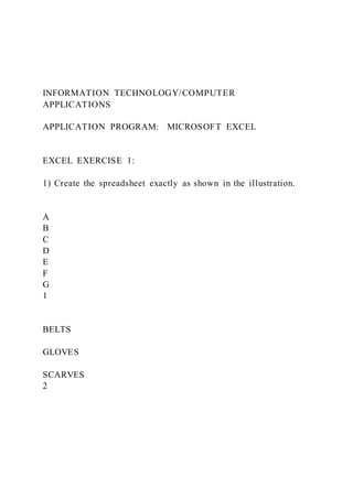
1) In a new spreadsheet enter the values exactly as shown in the
illustration.
A
B
6. 2) Save the document as PAYROLL in your folder.
EXCEL EXERCISE 3:
1) In a new spreadsheet enter the values exactly as shown in the
illustration.
A
B
C
D
E
F
G
1
January
February
March
1st QTR.
11. 20
SAVINGS
2) Save as BUDGET.
EXCEL EXERCISE 4:
1) In a new spreadsheet enter the values exactly as shown in the
illustration.
A
B
C
D
E
F
G
1
STOCK
UNIT OF
UNITS
COST PER
TOTAL
2
14. 3) Enter the missing information for Unit of Count as indicated:
a. The UNIT Of COUNT for Pencils, Staples, Clips, and Disks
is Box.
b. The UNIT Of COUNT for Staplers, and Ribbons is Each.
4) Save the document as INVEN in your folder.