Decision analysis problems online 1

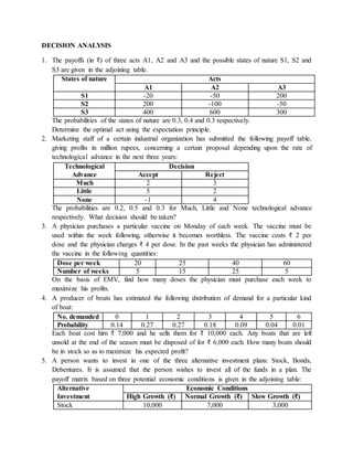
1. DECISION ANALYSIS
1. The payoffs (in ₹) of three acts A1, A2 and A3 and the possible states of nature S1, S2 and
S3 are given in the adjoining table.
States of nature Acts
A1 A2 A3
S1 -20 -50 200
S2 200 -100 -50
S3 400 600 300
The probabilities of the states of nature are 0.3, 0.4 and 0.3 respectively.
Determine the optimal act using the expectation principle.
2. Marketing staff of a certain industrial organization has submitted the following payoff table,
giving profits in million rupees, concerning a certain proposal depending upon the rate of
technological advance in the next three years:
Technological
Advance
Decision
Accept Reject
Much 2 3
Little 5 2
None -1 4
The probabilities are 0.2, 0.5 and 0.3 for Much, Little and None technological advance
respectively. What decision should be taken?
3. A physician purchases a particular vaccine on Monday of each week. The vaccine must be
used within the week following, otherwise it becomes worthless. The vaccine costs ₹ 2 per
dose and the physician charges ₹ 4 per dose. In the past weeks the physician has administered
the vaccine in the following quantities:
Dose per week 20 25 40 60
Number of weeks 5 15 25 5
On the basis of EMV, find how many doses the physician must purchase each week to
maximize his profits.
4. A producer of boats has estimated the following distribution of demand for a particular kind
of boat:
No. demanded 0 1 2 3 4 5 6
Probability 0.14 0.27 0.27 0.18 0.09 0.04 0.01
Each boat cost him ₹ 7,000 and he sells them for ₹ 10,000 each. Any boats that are left
unsold at the end of the season must be disposed of for ₹ 6,000 each. How many boats should
be in stock so as to maximize his expected profit?
5. A person wants to invest in one of the three alternative investment plans: Stock, Bonds,
Debentures. It is assumed that the person wishes to invest all of the funds in a plan. The
payoff matrix based on three potential economic conditions is given in the adjoining table:
Alternative
Investment
Economic Conditions
High Growth (₹) Normal Growth (₹) Slow Growth (₹)
Stock 10,000 7,000 3,000

2. Bonds 8,000 6,000 1,000
Debentures 6,000 6,000 6,000
Determine the best investment plan using each of the following criteria:
(i) Laplace, (ii) Maximin, (iii) Maximax
6. Given is the following payoff matrix
States of Nature Probability Courses of Action
Do not expand Expand 200
units
Expand 400
units
High Demand 0.4 2,500 3,500 5,000
Medium Demand 0.4 2,500 3,500 2,500
Low Demand 0.2 2,500 1,500 1,000
What should be the decision if we use: (i) EMV criterion, (ii) The Maximin criterion, (iii)
The maximax criterion, (iv) Minimax regret criterion?
7. The research director of XYZ Pharmaceutical Laboratory has to decide about one of three
influenza vaccines (P1, P2, P3) which should be funded for mass production. Payoffs depend
upon the type of influenza outbreak (S1, S2, S3, S4) that is most persuasive in the next year.
The payoff matrix, with profits (in millions of rupees), is given below:
States of Nature Courses of Action
P1 P2 P3
S1 10 8 -15
S2 4 12 12
S3 0 -5 8
S4 -2 -10 8
Prior to acquiring any additional information about the occurrence of states of nature, the
director’s probability judgements are: P(S1) = 0.2 and P(S2) = 0.2, P(S3) = 0.5 and P(S4) =
0.1.
(i) If the director could consult an authority who could tell him which state will occur,
what is the expected value of this information using above payoff matrix.
(ii) Verify your answer by calculating EVPI from the loss matrix.
8. An executive has to make a decision. He has four alternatives D1, D2, D3 and D4. When the
decision has been made events may lead such that any of the four results may occur. The
results are R1, R2, R3 and R4. Probabilities of occurrence of these results are as follows:
R1 = 0.5, R2 = 0.2, R3 = 0.2 and R4 = 0.1
The matrix of payoff between the decision and the results is indicated in the adjoining table:
R1 R2 R3 R4
D1 14 9 10 5
D2 11 10 8 7
D3 9 10 10 11
D4 8 10 11 13
Show this decision situation in the form of a decision tree and indicate the most preferred
decision and corresponding expected value.

3. 9. A Finance Manager is considering drilling a well. In the past, only 70% of wells drilled were
successful at 20 metres depth in that area. Moreover on finding no water at 20 metres, some
persons in that area drilled it further up to 25 metres but only 20 % struck
10. Expected return (in million rupees) from the sale of three machines A, B and C under
expected market condition as poor (S1), Fair (S2) and Good (S3) are given in the following
table below:
Sales Courses of Action
Poor (S1) Fair (S2) Good (S3)
S1 0.5 1.0 1.5
S2 0 1.5 2.5
S3 -1.5 0.5 3.5
Chance of market at states S1, S2 and S3 are 30%, 50% and 20% respectively. But the
market research finds the actual chances of states of market as follows:
Actual State M1 (Poor) M2 (Fair) M3 (Good)
S1 0.7 0.2 0.1
S2 0.2 0.7 0.1
S3 0 0.2 0.8
Find (i) Conditional expected loss table
(ii) Expected Value of Perfect Information (EVPI).
(iii) Expected loss table on the basis of the results of market research.
(iv) Economic cost of market research
Illustration
Suppose a electrical good has a resource base to buy for resale purposes in a market, electric
irons in the range of 0 to 4. His resource base permits him to buy nothing or 1 or 2 or 3 or 4
units. These are his alternative courses of action or strategies. The demand for electric irons in
any month is something beyond his control and hence is a state of nature. Let us presume that the

4. dealer does not know how many units will be bought from him by the customers. The demand
could be anything from 0 to 4. The dealer can buy each unit of electric iron @ ₹ 40 and sell it at
₹ 45 each, his margin being ₹ 5 per unit. Assume the stock on hand is valueless. Portray in a
payoff table the EMV.
COMPUTATION OF EXPECTED MONETRAY VALUE (EMV)
States
of
nature
Probability Conditional Payoff (₹)
Courses of action
Expected Payoff (₹)
Courses of action
A1(0) A2(1) A3(2) A4(3) A5(4) A1(0) A2(1) A3(2) A4(3) A5(4)
(1) (2) (3) (4) (5) (6) (1) x
(2)
(1) x
(3)
(1) x
(4)
(1) x
(5)
(1) x
(6)
S1(0) 0.04 0 -40 -80 -120 -160 0 -1.6 -3.2 -4.8 -6.4
S2(1) 0.06 0 5 -35 -75 -115 0 0.30 -2.1 -4.5 -6.9
S3(2) 0.20 0 5 10 -30 -70 0 1.0 2.0 -6.0 -14.0
S4(3) 0.30 0 5 10 15 -25 0 1.5 3.0 4.5 -7.5
S5(4) 0.40 0 5 10 15 20 0 2.0 4.0 6.0 8.0
EMV 0 3.2 3.7 -4.8 -26.8
Conditional payoff value = (Marginal profit (Units sold) – (Marginal Loss) (Units not sold)
= (₹ 45 - ₹ 40) (Units sold) – (₹ 40)(Units not sold)
PAYOFF AND REGRET TABLE
States of
nature
(Probable
Demand)
Conditional Payoff (₹)
Courses of action (Strategies
Possible Supply)
Conditional Opportunity Loss (₹)
Courses of action (Strategies Possible Supply)
0 1 2 3 4 0 1 2 3 4
0 0 -40 -80 -120 -160 0 0 – (-40) = 40 0 – (-80) = 80 0 – (-120) = 120 0 – (-160) = 160
1 0 5 -35 -75 -115 5 – 0 = 5 5 – 5 = 0 5 – (-35) = 40 5 – (-75) = 80 5 – (-115) = 120
2 0 5 10 -30 -70 10 – 0 = 10 10 – 5 = 5 10 – 10 = 0 10 – (-30) = 40 10 – (-70) = 80
3 0 5 10 15 -25 15 – 0 = 15 15 – 5 = 10 15 – 10 = 5 15 – 15 = 0 15 – (-25) = 40
4 0 5 10 15 20 20 – 0 = 20 20 – 5 = 15 20 – 10 = 10 20 – 15 = 5 20 – 20 = 0
States of
nature
Probability Conditional Opportunity Loss (₹) Expected Opportunity Loss (₹)
Courses of action
0 1 2 3 4 0 1 2 3 4
0 0.04 0 40 80 120 160 0 1.6 3.2 4.8 6.4
1 0.06 5 0 40 80 120 0.3 0 2.4 4.8 7.2
2 0.20 10 5 0 40 80 2 1 0 8 16
3 0.30 15 10 5 0 40 4.5 3 1.5 0 12
4 0.40 20 15 10 5 0 8 6 4 2 0
Expected Opportunity Loss (EOL) 14.8 11.6 11.1 19.6 41.6
Decision Making under Uncertainty
Maximin
States of Nature
(Possible Demand)
Courses of Action (Possible Supply)
A1: 0 A2: 1 A3: 2 A4: 3 A5: 4
S1: 0
S2: 1
S3: 2
S4: 3
S5: 4
Minimum in

5. columns
Solutions
1. COMPUTATION OF EXPECTED MONETRAY VALUE (EMV)
States
of
Nature
(Sj)
Probability
P(S)
Conditional Payoff(₹)
Acts
Expected Payoff (₹)
Acts
A1 A2 A3 A1 A2 A3
S1 0.3 -20 -50 200 -6 -15 60
S2 0.4 200 -100 -50 80 -40 -20
S3 0.3 400 600 300 120 180 90
Expected Monetary Value (EMV) 194 125 130
The maximum value of EMV is corresponding to act A1. Hence, according to the EMV
criterion, the optimal act is A1.
2. COMPUTATION OF EMV FOR VARIOUS ACTS
Technological
Advance
Probability Conditional Payoff Expected Payoff
Accepting Rejecting Accepting Rejecting
Much 0.2 2 3 0.4 0.6
Little 0.5 5 2 2.5 1.0
None 0.3 -1 4 -0.3 2.8
Expected Monetary Value (EMV) 2.6 2.8
Since EMV of rejecting the proposal is 2.8 which is more than EMV of accepting the
proposal, the decision should be ‘reject the proposal’.
5. Let HG: High Growth, NG: Normal Growth, SG: Slow Growth
PAYOFF TABLE (in Rupees)
Act
(Investment
States of nature Row
Minimum
Row
Maximum
Row
Total
S1:
HG
S2: NG S3: SG
(1) (2) (3) (4) (5) (6) (7)
A1: Stocks 10,000 7,000 3,000 3,000 10,000 20,000
A2: Bonds 8,000 6,000 1,000 1,000 8,000 15,000
A3: Debentures 6,000 6,000 6,000 6,000 6,000 18,000
Probability 1/3 1/3 1/3 Column (5)
Max. = 6,000
Column (6)
Max. = 10,000
(i) Laplace Criterion
EMV (A1: Stocks) = ₹ 1/3(10,000 + 7,000 + 3,000) = ₹ 20,000/3 = ₹ 6,666.67
EMV (A2: Bonds) = ₹ 1/3(8,000 + 6,000 + 1,000) = ₹ 15,000/3 = ₹ 5,000
EMV (A3: Debentures) = ₹ 1/3(6,000 + 6,000 + 6,000) = ₹ 18,000/3 = ₹ 6,000

6. Max. (EMV) = ₹ 6,666.67 which corresponds to acts A1. Hence, under Laplace criterion act
A1: Stock, can be taken as the optimal act.
(ii) Maximin Criterion
From column (5) of the above Table, we get
Maximum (Minimum Payoffs) = ₹ 6,000, which corresponds to act A3.
Hence, under the Maximin criterion, act A3: Debenture is the optimal choice
(iii) Maximax Criterion
From column (6) of the above Table, we get
Maximum (Maximum Payoffs) = ₹ 10,000, which corresponds to act A1.
Hence, under the Maximax criterion, act A1: Stock is the optimal choice
6. Payoff Table
Act
(Investment
Probability Conditional Payoff (₹)
Courses of action
Expected Payoff (₹)
Courses of action
A1: Do
not
expand
A2:
Expand
200 units
A3:
Expand
400 units
A1: Do
not
expand
A2:
Expand
200 units
A3:
Expand
400 units
(1) (2) (3) (4) (1) x (2) (1) x (3) (1) x (4)
S1: High
Demand
0.4 2,500 3,500 5,000 1,000 1,400 2,000
S2: Medium
Demand
0.4 2,500 3,500 2,500 1,000 1,400 1,000
S3: Low
Demand
0.2 2,500 1,500 1,000 500 300 200
EMV 2,500 3,100 3,200
Minimum Payoff (₹) 2,500 1,500 1,000
Maximum Payoff (₹) 2,500 3,500 5,000
(i) EMV criterion thus suggests that we should decide to expand 400 units since EMV
3,200 is highest.
(ii) In the maximin criterion the strategy for which minimum payoff is maximum is
chosen. The minimum payoff values corresponding to the strategies: Do not expand,
Expand 200 units, and Expand 400 units, are 2,500; 1,500 and 1,000 respectively. Of
these payoffs 2,500 is maximum which corresponds to the strategy ‘Do not expand’.
Therefore, a decision maker using Maximin criterion would decide ‘Not to expand’.
Overall maximum payoff values (due to high demand) are ₹ 5,000 that corresponds to
the act – Expand 400 units. By using maximax criterion the decision maker would
decide ‘Expanding 400 units’.
Minimax Regret:
In this criterion profits are transformed into opportunity losses (or regret). A regret
matrix is obtained from the payoff matrix by subtracting each of the values in a row
from the largest payoff value in the row. Under this approach the decision – maker
identifies the maximum regret for each act and selects the act due to which maximum

7. regret value is minimum. This may be achieved by selecting the act which maximum
regret (i.e. column maximum of the regret matrix) is minimum.
Regret matrix of the previous payoff matrix is as follows:
States of Nature Probability Courses of Action (Possible Supply)
A1: Do not
Expand
A2: Expand
200 units
A3: Expand 400
units
S1: High Demand 0.4 5,000 – 2,500 =
2,500
5,000 – 3,500 =
1,500
5,000 – 5,000 = 0
S2: Medium
Demand
0.4 3,500 – 2,500 =
1,000
3,500 – 3,500 =
0
3,500 – 2,500 =
1,000
S3: Low Demand 0.2 2,500 – 2,500 = 0 2,500 – 1,500 =
1,000
2,500 – 1,000 =
1,500
Maximum Regret 2,500 1,500 1,500
The decision – maker must choose ‘Expand 200 units’ or ‘Expand 400 units’ for it
minimizes the maximum possible return.
7. COMPUTATION OF EXPECTED PAYOFF
Act
(Investment
Probability Conditional Payoff (₹)
Courses of action
Expected Payoff (₹)
Courses of action
P1 P2 P3 P1 P2 P3
(1) (2) (3) (4) (1) x (2) (1) x (3) (1) x (4)
S1 0.2 10 8 -15 2.0 1.6 -3.0
S2 0.2 4 12 12 0.8 2.4 2.4
S3 0.5 0 -5 8 0 -2.5 4.0
S4 0.1 -2 -10 8 -0.2 -1.0 0.8
EMV 2.6 0.5 4.2
From the table, we find that the highest prior expected value is 4.2 (million rupees). Prior
expected value of selecting the optimal act after learning which state will occur
= 10 x 0.2 + 12 x 0.2 + 8 x 0.5 + 8 x 0.1 = 9.2
Expected value of perfect information = 9.2 – 4.2 = ₹ 5 million
8. Decision Tree Diagram
D1
D2
D3
D4
R1
R2
R3
R4

8. Monetary Value Prob. Expected Value EMV
D1
14 0.5 7.0
11.3
9 0.2 1.8
10 0.2 2.0
5 0.1 0.5
D2
11 0.5 5.5
9.8
10 0.2 2.0
8 0.2 1.6
7 0.1 0.7
D3
9 0.5 4.5
9.6
10 0.2 2.0
10 0.2 2.0
11 0.1 1.1
D4
8 0.5 4.0
9.5
10 0.2 2.0
11 0.2 2.2
13 0.1 1.3
The most preferred decision at the decision node 1 is found by calculating expected value of each decision branch
and selecting the path (course of action) with high value.
Since node D1 has the highest EMV, the decision at node A will be choose the course of action D1.
States of Nature Probability Courses of Action (Possible Supply)
A1: Do not
Expand
A2: Expand
200 units
A3: Expand 400
units
S1: High Demand 0.4 5,000 – 2,500 =
2,500
5,000 – 3,500 =
1,500
5,000 – 5,000 = 0
S2: Medium
Demand
0.4 3,500 – 2,500 =
1,000
3,500 – 3,500 =
0
3,500 – 2,500 =
1,000
S3: Low Demand 0.2 2,500 – 2,500 = 0 2,500 – 1,500 =
1,000
2,500 – 1,000 =
1,500
Maximum Regret 2,500 1,500 1,500
9. (i) (a) The conditional profit table is given below:
States of
Nature
Prior
Probability
Courses of Action (Buying Decision)
A B C
S1: Poor 0.30 0.5 0 -1.5
S2: Fair 0.50 1.0 1.5 0.5
S3: Good 0.20 1.5 2.5 3.5

9. (b) Subtracting the payoffs against each event from the largest payoffs (market*) gives the conditional
opportunity losses (COL) as shown in the table below:
Act
(Investment
Probability Conditional Loss (₹)
Courses of action
Expected Opportunity Loss (₹)
Courses of action
A B C A B C
S1 0.30 0 0.5 2.0 0 0.15 0.60
S2 0.50 0.5 0 1.0 0.25 0 0.50
S3 0.20 2.0 1.0 0 0.40 0.20 0
EMV 0.65 0.35 1.10
(ii) EOL for machine B is least (0.35). Under perfect information, the opportunity loss would be zero, so
the expected value under EVPI is 0.35.
(iii) The margin and joint prob. Is computed as under:
Act
(Investment
Probability Conditional Prob.
Courses of action
Joint Prob.
Courses of action
S1 0.30 0.7 0.2 0.1 0.21 0.06 0.03
S2 0.50 0.2 0.7 0.1 0.10 0.35 0.05
S3 0.20 0 0.2 0.8 0 0.04 0.16
Total P(M1)
= 0.31
P(M2) =
0.45
P(M3) =
0.24
Revising the prior prob with the help of Bayes’ Theorem, the reqd. posterior prob. Are computed as
below:
Outcome Prob. States of nature Posterior prob.
M1 0.31 S1 0.21/0.31 = 0.677
S2 0.10/0.31 = 0.323
S3 0/0.31 = 0
M2 0.45 S1 0.06/0.45 = 0.133
S2 0.35/0.45 = 0.778
S3 0.04/0.45 = 0.089
M3 0.24 S1 0.03/0.24 = 0.125
S2 0.05/0.24 = 0.208
S3 0.16/0.24 = 0.667
Act
(Investment
I II
Prob COL EOL A B C
S1 0 0.5 2.0 0 0.15 0.60
S2 0.5 0 1.0 0.25 0 0.50
S3 2.0 1.0 0 0.40 0.20 0