SlideShare a Scribd company logo
1 of 71
You clearly understand the concepts of this assignment. You’ve
done an excellent job answering the problems correctly. You’ve
demonstrated a clear understanding of stats and their
application to this assignment. You read your diagrams and
explained the results correctly, and your formulaic work at the
end is right on target. You have also written a very clean,
narrative document.
Be sure to look at the formatting of your sources. Be sure to
always use credible sources to back your work. This is so
important when it comes to academic and scholarly work. Please
see my comments throughout the paper. That’s really where the
advice ends regarding things you should work on, because you
have demonstrated you have no problems with the content.
Knowing these concepts, and progressing even more toward an
academic writing style, will help you as you move forward
personally and professionally. Being able to translate numbers
into a sharp narrative document will make you a go-to person in
the workplace, and it will provide confidence in everything you
do. Good work on this assignment.
Chapter Seven
Problem 1) Look at the scatterplot below. Does it demonstrate
a positive or negative correlation? Why?
Are there any outliers? What are they?
The scatterplot is an example of a positive correlation, the
outlier in the scatterplot is 6.00. A ; “Outliners are a set of data,
a value so far removed from other values in the distribution that
its presence cannot be attributed to the random combination of
chance causes” (http://www.statcan.gc.ca/,2013)scatterplot is
considered positive when the point runs from the lower left to
the upper right such as the circles shown on the example
.
Problem 2) Look at the scatterplot below. Does it demonstrate
a positive or negative correlation? Why?
Are there any outliers? What are they?
The scatter plot is the opposite of example one, it is actually a
negative correlation
because the points run from the upper left to the lower right.
As with example one there is an outer liner which is 6.00 as
well, it does not fall within line with the other points.
Problem 3) The following data come from your book, problem
26 on page 298. Here is the data:
Mean daily calories Infant Mortality Rate (per 1,000 births)
1523 154
3495 6
1941 114
2678 24
1610 107
3443 6
1640 153
3362 7
3429 44
2671 7
For the above data construct a scatterplot using SPSS or Excel
(Follow instructions on page 324 of your textbook). What does
the scatterplot show? Can you determine a type of relationship?
Are there any outliers that you can see?
Mean daily calories
Infant Mortality Rate
(per 1,000 births)
1523
154
3495
6
1941
114
2678
24
1610
107
3443
6
1640
153
3362
7
3429
44
2671
7
Infant Mortality Rate (per 1,000 births)
0
20
40
60
80
100
120
140
160
180
020004000
Infant Mortality
Rate (per 1,000
births)
The scatter plot demonstrates that there is a significant
reverence between the number of calories and the infant
mortality rate; according to the plot if the calorie intake were to
increase there would be a decrease in the infant mortality rate.
Because the points flow from the upper left to the lower right
they show that the correlation is negative. The outliners are
demonstrated as a calorie intake of 3,429 and the infant
mortality rate of 44, and also a calorie rate of 2,671 and an
infant mortality rate of 7.
b) Using the same data conduct a correlation analysis using
SPSS or Excel. What is the correlation coefficient? Is it a
strong, moderate or weak correlation? Is the correlation
significant or not? If it is what does that mean?
Excel shows a correlation coefficient of -.9, because of this it is
considered to be strong, if the number would have been closer
to 0 it would have been considered weak. “The correlation
coefficient is a number between -1 and 1, If one variable
increases when the second one increases, then there is a positive
correlation. In this case the correlation coefficient will be closer
to 1; If one variable decreases when the other variable
increases, then there is a negative correlation and the
correlation coefficient will be closer to -1” (www.medcalc.org,
2014). The correlation shows significant because the data is -9,
therefore the calorie intake of infants is very important to their
survival.
Problem 4)
Bill is doing a project for you in the marketing department. In
conducting his analysis regarding consumer behavior and a new
product that has come out, he tells you the correlation between
these two variables is 1.09. What is your response to this
analysis?
I would know that Bill has made a mistake somewhere in his
analysis because there is no such correlation of 1.09 they are
measured from -1 to +1
.
Problem 5)
Judy has conducted an analysis for her supervisor. The result
she obtained was a correlation coefficient that was negative
0.86. Judy is confused by this number and feels that because it
is negative and not positive is means that it is bad. You are her
supervisor. How would you clarify this result for Judy regarding
the meaning of the correlation?
I would explain to Judy that when dealing with correlations
looks can be deceiving and just because a result may be
considered negative it does not necessarily mean less.
“Although it seems correlation is fairly obvious your data may
contain unsuspected correlations. You may also suspect there
are correlations, but don't know which are the strongest”
(www.surveysystems.com, 2012). I would also explain to Judy
that the fact that the analysis shows negative only means that
it’s variables move in opposite directions.
Problem 6)
Explain the statement, “correlation does not imply causality.”
Simply put the statement means one variable does not cause the
other, there may be times that it would seem likely but there is
probable that there is some other reason. (Prinston
.edu, 2012).
Problem 7)
Using the best-fit line below for prediction, answer the
following questions:
What would you predict the price of Product X in volume of 150
to be (approximately)?
I predict the price of Product X in volume of 150 would be
250.00. If you draw a line to the 150.00 volume to the best fit
line and then to the price axis it indicates 250.00
What would you predict the price of Product X in volume of 100
to be (approximately)?
The prediction for Product X in volume of 100 would be 175.00,
draw a line from the 100.00 volume to the best fit line and then
the price axis and it indicates 175.00.
Problem 8)
You are interested in finding out if a student’s ACT score is a
good predictor of their final college grade point average (GPA).
You have obtained the following data and are going to conduct
a regression analysis. Follow instructions on page 324 of your
textbook under line of best fit to conduct this analysis.
ACT
GPA
22.0
3.0
2.0
3.78
33.0
3.68
21.0
2.94
27.0
3.38
25.0
3.21
30.0
3.65
What is the R? What type of relationship does it indicate
(strong/weak; positive/negative)?
22
3.00
32
3.78
33
3.68
21
2.94
27
3.38
25
3.21
30
3.65
r =
0.984275
0.00
0.50
1.00
1.50
2.00
2.50
3.00
3.50
4.00
05101520253035
The relationship between the ACT and the GPA is strong, with
the r being r=0.98. The point also goes from the lower left to
the upper right.
Go to the coefficients readout. The constant is the intercept.
Under that is the ACT and that is the slope. Using the straight
line formula of Y = mx + b, which you will find on page 313,
you will now predict some future GPA scores: In the formula
(m) is the slope; (x) is the variable that you are looking to use
as a predictor; and (b) is the intercept. Predict GPA from the
following ACT scores using the regression equation/straight
line formula (show all your work):
Using the formula x=mx + b, the slope (m-value) is
0.070391949152542 and the intercept (b-value)
1.4665042372881; x is the variable and will be used as the
predictor. In order to get the GPA both the m-value and b value
will be rounded off making the GPA:
20
Y = mx+b
Y = 0.0704(20) + 1.4665
Y = 1.408 + 1.4665
Y = 2.8745
Y=2.78
25
Y = mx+b
Y = 0.0704(25) + 1.4665
Y = 1.76 + 1.4665
Y = 3.2265
Y = 3.23
34
Y = mx+b
Y = 0.0704(34) + 1.4665
Y = 2.3936 + 1.4665
Y = 3.8601
Y = 3.86
Chapter Eight
Show all your work
Problem 1) A sample of nine students is selected from among
the students taking a particular exam. The nine students were
asked how much time they had spent studying for the exam and
the responses (in hours) were as follows:
�Correct. Be sure to cite your sources in proper APA. Why do
you suppose it’s so important to back your work with credible
sources?
�Very good.
�Be sure to cite academic sources in each section.
�Again, find academic sources. Peer reviewed is essential.
�Correct. Same comment re: credible sources.
�These are correct.
Slide 10 - *
Active Learning Questions
Copyright © 2009 Pearson Education, Inc.
For use with classroom response systems
Chapter 10
t Tests, Two-Way Tables,
and ANOVA
*
Slide 10 - *
This partial t-table can be used where necessary.
*
Slide 10 - *
The t distribution can be used when finding a confidence
interval for the population mean with a small sample whenever
the sample comes from a symmetric population.
a. True
b. False
*
Slide 10 - *
The t distribution can be used when finding a confidence
interval for the population mean with a small sample whenever
the sample comes from a symmetric population.
a. True
b. False
*
Slide 10 - *
A simple random sample from a normal distribution is taken in
order to obtain a 95% confidence interval for the population
mean. If the sample size is 12, the sample mean is 32, and the
sample standard deviation s is 9.5, what is the margin of error?
a. 0.604
b. 1.74
c. 5.98
d. 6.04
*
Slide 10 - *
A simple random sample from a normal distribution is taken in
order to obtain a 95% confidence interval for the population
mean. If the sample size is 12, the sample mean is 32, and the
sample standard deviation s is 9.5, what is the margin of error?
a. 0.604
b. 1.74
c. 5.98
d. 6.04
*
Slide 10 - *
A 95% confidence interval for the mean of a normal population
a. 0.8
b. 0.16
c. 1.6
d. 16
*
Slide 10 - *
A 95% confidence interval for the mean of a normal population
is found
a. 0.8
b. 0.16
c. 1.6
d. 16
*
Slide 10 - *
The margin of error in estimating the population mean of a
normal population is E = 9.3 when the sample size is 15. If the
sample size had been 6 and the sample standard deviation did
not change, how would the margin of error change?
a. It would be smaller
b. It would be larger
c. It would stay the same
d. Cannot be determined
*
Slide 10 - *
A golfer wished to find a ball that would travel more than 200
yards when hit with his 4-iron with a club speed of 90 miles per
hour. He had a golf equipment lab test a low compression ball
by having a robot swing his club 9 times at the required speed.
State the null and alternative hypotheses for this test.
a.
b.
c.
d.
*
Slide 10 - *
Data from the test in the previous example resulted in a sample
mean of 206.8 yards with a sample standard deviation of 4.6
yards. Assuming normality, find the value of the t statistic.
Recall the mean being tested was 200 yards with 9 swings by
the robot.
a. –4.435
b. –13.304
c. 4.435
d. 13.304
*
Slide 10 - *
Data from the test in the previous example resulted in a sample
mean of 206.8 yards with a sample standard deviation of 4.6
yards. Assuming normality, find the critical value at the 0.05
significance level. Recall the mean being tested was 200 yards
with 9 swings by the robot.
a. 2.306
b. 2.262
c. 1.833
d. 1.860
*
Slide 10 - *
For the previous example, determine the results of a hypothesis
test.
a. Reject the null hypothesis. The data provide sufficient
evidence that the average distance is greater than 200 yards.
b. Accept the null hypothesis. The data provide sufficient
evidence that the average distance is greater than 200 yards.
c. Reject the null hypothesis. The data do not provide
sufficient evidence that the average distance is greater than 200
yards.
d. Accept the null hypothesis. The data do not provide
sufficient evidence that the average distance is greater than 200
yards.
*
Slide 10 - *
One hundred people are selected at random and tested for
colorblindness to determine whether gender and colorblindness
are independent. The following counts were observed. Find the
expected value of a male who is not colorblind.
a. 6.0 b. 54.0
c. 4.0 d. 36.0ColorblindNot
ColorblindTotalMale95160Female13940Total1090100
*
Slide 10 - *
One hundred people are selected at random and tested for
colorblindness to determine whether gender and colorblindness
are independent. The following counts were observed. Find the
expected value of a male who is not colorblind.
a. 6.0 b. 54.0
c. 4.0 d. 36.0
ColorblindNot
ColorblindTotalMale95160Female13940Total1090100
*
Slide 10 - *
For the previous example, here are the expected values. Find the
a. 1.389 b. 1.0
c. 4.167 d. 4.0ColorblindNot
ColorblindTotalMale6.054.060Female4.036.040Total10.090.010
0
*
Slide 10 - *
For the previous example, here are the expected values. Find the
a. 1.389 b. 1.0
c. 4.167 d. 4.0
ColorblindNot
ColorblindTotalMale6.054.060Female4.036.040Total10.090.010
0
*
Slide 10 - *
State the null and alternative hypothesis for the test associated
with the data in the previous example.
a. H0: Colorblindness and gender are independent
Ha: Colorblindness and gender are related
b. H0: Colorblindness and gender are dependent
Ha: Colorblindness and gender are not related
c. H0: Colorblindness and gender are related
Ha: Colorblindness and gender are independent
d. H0: Colorblindness and gender are nor related
Ha: Colorblindness and gender are dependent
*
Slide 10 - *
the previous example had been 4.216, state your conclusion
about the relationship between gender and colorblindness.
a. Reject H0. There is insufficient evidence to support the
claim that colorblindness and gender are related.
b. Accept H0. There is insufficient evidence to support the
claim that colorblindness and gender are related.
c. Reject H0. There is sufficient evidence to support the
claim that colorblindness and gender are related.
d. Accept H0. There is sufficient evidence to support the
claim that colorblindness and gender are related.
*
Slide 10 - *
able using a 0.05
the previous example had been 4.216, state your conclusion
about the relationship between gender and colorblindness.
a. Reject H0. There is insufficient evidence to support the
claim that colorblindness and gender are related.
b. Accept H0. There is insufficient evidence to support the
claim that colorblindness and gender are related.
c. Reject H0. There is sufficient evidence to support the
claim that colorblindness and gender are related.
d. Accept H0. There is sufficient evidence to support the
claim that colorblindness and gender are related.
*
Slide 10 - *
The data given were analyzed using one-way analysis or
variance. The purpose of the analysis is to:
a. determine whether the groups A, B, and C are independent.
b. test the hypothesis that the population means of the three
groups are equal.
c. test the hypothesis that the population variances of the
three groups are equal.
d. test the hypothesis that the sample means of the three
groups are equal.ABC292719262321252925282117
*
Slide 10 - *
The data given were analyzed using one-way analysis or
variance. The purpose of the analysis is to:
a. determine whether the groups A, B, and C are independent.
b. test the hypothesis that the population means of the three
groups are equal.
c. test the hypothesis that the population variances of the
three groups are equal.
d. test the hypothesis that the sample means of the three
groups are equal.
ABC292719262321252925282117
*
Slide 10 - *
Here are the results of the ANOVA for the previous example
(question on next
slide):SUMMARYGroupsCountSumsAverageVarianceA4108273
.33333B41002513.33333C48220.511.66667SUMMARYSource
of VariationSSdfMSFP-valueF critBetween
Groups88.7244.34.6940.04014.25649Within
Groups8599.4Total173.711
*
Slide 10 - *
If the significance level for the test is 0.05, which conclusion
below is correct?
a. The data do not provide sufficient evidence to conclude
that the population means of groups A, B, and C are related.
b. The data do not provide sufficient evidence to conclude
that the population means of groups A, B, and C are different.
c. The data do not provide sufficient evidence to conclude
that the population variances of groups A, B, and C are
different.
d. The data do not provide sufficient evidence to conclude
that the population means of groups A, B, and C are different.
*
x
Slide 9 - *
Active Learning Questions
Copyright © 2009 Pearson Education, Inc.
For use with classroom response systems
Chapter 9
Hypothesis Testing
*
Slide 9 - *
Note: Students should have their textbooks open to page 211 in
the textbook and refer to Table 5.1 when answering these Active
Learning Questions.
*
Slide 9 - *
A researcher claims that less than 62% of voters favor gun
control. State the null hypothesis and the alternative hypothesis
for a test of significance.
a. H0: p = 0.62 Ha: p > 0.62
b. H0: p < 0.62 Ha: p = 0.62
c. H0: p > 0.62 Ha: p = 0.62
d. H0: p = 0.62 Ha: p < 0.62
*
Slide 9 - *
A researcher claims that less than 62% of voters favor gun
control. State the null hypothesis and the alternative hypothesis
for a test of significance.
a. H0: p = 0.62 Ha: p > 0.62
b. H0: p < 0.62 Ha: p = 0.62
c. H0: p > 0.62 Ha: p = 0.62
d. H0: p = 0.62 Ha: p < 0.62
*
Slide 9 - *
A study of a brand of “in the shell” peanuts gives the following
table. A significant event at the 0.01 level is a fan getting a bag
with how many peanuts?
a. 25, 30, or 35 b. 25, 30, or 55
c. 35, 45, or 50 d. None of the choices# Peanuts in the
bag25303540455055Probability0.0030.020.090.150.450.2170.07
*
Slide 9 - *
A study of a brand of “in the shell” peanuts gives the following
table. A significant event at the 0.01 level is a fan getting a bag
with how many peanuts?
a. 25, 30, or 35 b. 25, 30, or 55
c. 35, 45, or 50 d. None of the choices
# Peanuts in the
bag25303540455055Probability0.0030.020.090.150.450.2170.07
*
Slide 9 - *
The manufacturer of a refrigerator system for beer kegs
produces refrigerators that are supposed to maintain a true mean
temperatur
pilsner. The owner of the brewery does not agree with the
refrigerator manufacturer, and claims that the true mean
temperature is incorrect. Assume that a hypothesis test of the
claim has been conducted and that the conclusion of the test was
to reject the null hypothesis. Identify the population to which
the results of the test apply.
a. All refrigerators produced by the manufacturer specifically
to cool kegs of a particular German pilsner beer
b. All refrigerators produced by the manufacturer
c. All refrigerators produced by the manufacturer specifically
to cool kegs of beer
d. There is not sufficient description to identify the
population
*
Slide 9 - *
The manufacturer of a refrigerator system for beer kegs
produces refrigerators that are supposed to maintain a true mean
pilsner. The owner of the brewery does not agree with the
refrigerator manufacturer, and claims that the true mean
temperature is incorrect. Assume that a hypothesis test of the
claim has been conducted and that the conclusion of the test was
to reject the null hypothesis. Identify the population to which
the results of the test apply.
a. All refrigerators produced by the manufacturer specifically
to cool kegs of a particular German pilsner beer
b. All refrigerators produced by the manufacturer
c. All refrigerators produced by the manufacturer specifically
to cool kegs of beer
d. There is not sufficient description to identify the
population
*
Slide 9 - *
A cereal company claims that the mean weight of the cereal in
its packets is at least 14 oz. Assume that a hypothesis test of the
claim has been conducted and that the conclusion of the test was
to reject the null hypothesis. Identify the population to which
the results of the test apply.
a. The cereal packets that were tested
b. The cereal packets of one kind manufactured by the cereal
company
c. The cereal packets claiming a weight of at least 14 oz
d. All cereal packets manufactured by the cereal company
*
Slide 9 - *
In 1990, the average math SAT score for students at one school
was 510. Five years later, a teacher wants to perform a
hypothesis test to determine whether the average math SAT
score of students at the school has changed from the 1990 mean
of 510. Formulate the null and alternative hypotheses for the
study described.
a.
b.
c.
d.
*
Slide 9 - *
The manufacturer of a refrigerator system for beer kegs
produces refrigerators that are supposed to maintain a true mean
pilsner. The owner of the brewery does not agree with the
refrigerator manufacturer, and claims he can prove that the true
mean temperature is incorrect. Assuming that a hypothesis test
of the claim has been conducted and that the conclusion is to
reject the null hypothesis, state the conclusion in non-technical
terms.
a. There is not sufficient evidence to support the claim that
the mean temperature is equal to 46ºF
b. There is sufficient evidence to support the claim that the
mean temperature is equal to 46ºF
c. There is not sufficient evidence to support the claim that
the mean temperature is different from 46ºF
d. There is sufficient evidence to support the claim that the
mean temperature is different from 46ºF
*
Slide 9 - *
-
value, determine whether the alternate hypothesis is supported
and give a reason for your conclusion.
a. Ha is not supported; is less than 1 standard deviation
above the claimed area
b. Ha is not supported; is more than 4 standard deviations
above the claimed area
c. Ha is supported; is less than 1 standard deviation above
the claimed area
d. Ha is supported; is more than 4 standard deviations
above the claimed area
*
Slide 9 - *
z = – -value for the
test?
a. 6.68
b. 93.32
c. 0.0668
d. None of the above
*
Slide 9 - *
z = – aimed value; What is the P-value for the
test?
a. 6.68
b. 93.32
c. 0.0668
d. None of the above
*
Slide 9 - *
A health insurer has determined that the “reasonable and
customary” fee for a certain medical procedure is $1200. They
suspect that the average fee charged by one particular clinic for
this procedure is higher than $1200. The insurer wants to
perform a hypothesis test to determine whether their suspicion
is correct. The mean fee charged by the clinic for a random
sample of 65 patients receiving this procedure was $1280. Do
the data provide sufficient evidence to conclude that the mean
fee charged by this particular clinic is higher than $1200? Use a
significance level of 0.01. Assume that σ = $220.
a. The z-score of 2.93 provides sufficient evidence to
conclude that the mean fee charged for the procedure is greater
than $1200
b. The z-score of 0.363 does not provide sufficient evidence
to conclude that the mean fee charged for the procedure is
greater than $1200
c. The P-value of 0.363 does not provide sufficient evidence
to conclude that the mean fee charged for the procedure is
greater than $1200
d. The P-value of 0.045 provides sufficient evidence to
conclude that the mean fee charged for the procedure is greater
than $1200
*
Slide 9 - *
A long-distance telephone company claims that the mean
duration of long-distance telephone calls originating in one
town was not equal to 9.4 minutes, which is the average for the
state. Determine the null and alternative hypotheses for the test
described.
a.
b.
c.
d.
*
Slide 9 - *
A long-distance telephone company claims that the mean
duration of long-distance telephone calls originating in one
town was not equal to 9.4 minutes, which is the average for the
state. Determine the null and alternative hypotheses for the test
described.
a.
b.
c.
d.
*
Slide 9 - *
A manufacturer wishes to test the claim that one of its pancake
mixes has a mean weight that does not equal 24 ounces as
advertised. Determine the conclusion of the hypothesis test
assuming that the results of the sampling lead to rejection of the
null hypothesis.
a. Support the claim that the mean is greater than 24 oz
b. Support the claim that the mean is not equal to 24 oz
c. Support the claim that the mean is equal to 24 oz
d. Support the claim that the mean is less than 24 oz
*
Slide 9 - *
The standard score for a two-tailed test is 2.0. What is the P-
value?
a. 0.9772
b. 0.0456
c. 0.0228
d. 97.72
*
Slide 9 - *
The standard score for a two-tailed test is 2.0. What is the P-
value?
a. 0.9772
b. 0.0456
c. 0.0228
d. 97.72
*
Slide 9 - *
A two-tailed test is conducted at the 5% significance level.
What is the smallest z-score listed below that results in
rejection of the null hypothesis?
a. 1.17
b. 1.58
c. 1.81
d. 2.89
*
Slide 9 - *
A two-tailed test is conducted at the 5% significance level.
What is the smallest z-score listed below that results in
rejection of the null hypothesis?
a. 1.17
b. 1.58
c. 1.81
d. 2.89
*
Slide 9 - *
A two-tailed test is conducted at the 10% significance level.
What is the z-score closest to zero in the list that will result in
rejection of the null hypothesis?
a. 1.19
b. –1.54
c. –1.84
d. 2.59
*
Slide 9 - *
A two-tailed test is conducted at the 10% significance level.
What is the z-score closest to zero in the list that will result in
rejection of the null hypothesis?
a. 1.19
b. –1.54
c. –1.84
d. 2.59
*
Slide 9 - *
In 1990, the average duration of long-distance telephone calls
originating in one town was 9.4 minutes. A telephone company
wants to perform a hypothesis test to determine whether the
average duration of long-distance phone calls has changed. The
mean duration for a random sample of 50 calls originating in the
town was 8.6 minutes. Does the data provide sufficient evidence
significance level 0.01, & σ = 4.2 minutes.
a. P-value greater than 0.01; sufficient evidence to accept the
null hypothesis and conclude that the mean call duration has
changed
b. P-value less than 0.01; sufficient evidence to reject the
null hypothesis and conclude that the mean call duration has
changed
c. P-value greater than 0.01; insufficient evidence to reject
the null hypothesis and conclude that the mean call duration has
changed
d. P-value greater than 0.01; sufficient evidence to reject the
null hypothesis and conclude that the mean call duration has
changed
*
Slide 9 - *
At one school, the average amount of time that tenth-graders
spend watching television each week is 21 hours. The principal
introduces a campaign to encourage the students to watch less
television. One year later, the principal wants to perform a
hypothesis test to determine whether the average amount of time
spent watching television per week has decreased. The
that the results of the sampling lead to non-rejection of the null
hypothesis. Classify that conclusion as a Type I error, a Type II
error, or a correct decision, if in fact the mean amount of time,
a. Type I error b. Correct decision c. Type II error
*
Slide 9 - *
A health insurer has determined that the “reasonable and
customary” fee for a certain medical procedure is $1200. They
suspect that the average fee charged by one particular clinic for
this procedure is higher than $1200. The insurer wants to
perform a hypothesis test to determine whether their suspicion
Explain the meaning of a correct decision.
a.
b.
c.
d.
*
Slide 9 - *
The average diastolic blood pressure of a group of men
suffering from high blood pressure is 96 mmHg. During a
clinical trial, the men receive a medication, which it is hoped,
will lower their blood pressure. After three months, the
researcher wants to perform a hypothesis test to determine
whether the average diastolic blood pressure of the men has
a.
b. Fa
c.
d.
*
Slide 9 - *
The average diastolic blood pressure of a group of men
suffering from high blood pressure is 96 mmHg. During a
clinical trial, the men receive a medication, which it is hoped,
will lower their blood pressure. After three months, the
researcher wants to perform a hypothesis test to determine
whether the average diastolic blood pressure of the men has
a.
b. Failing to
c.
d.
*
Slide 9 - *
A random sample of 139 forty-year-old men contains 26%
smokers. Use Table 5.1 to estimate the P-value for a test of the
claim that the percentage of forty-year-old men that smoke is
22%.
a. 0.2542
b. 0.1401
c. 0.2802
d. 0.1271
*
Slide 9 - *
A random sample of 139 forty-year-old men contains 26%
smokers. Use Table 5.1 to estimate the P-value for a test of the
claim that the percentage of forty-year-old men that smoke is
22%.
a. 0.2542
b. 0.1401
c. 0.2802
d. 0.1271
*
Slide 9 - *
According to a recent poll 53% of Americans would vote for the
incumbent president. If a random sample of 100 people results
in 45% who would vote for the incumbent, test the hypothesis
that the actual percentage is 53%. Use a 0.10 significance level
and a two-tailed test.
a. Do not reject the null hypothesis; insufficient evidence to
reject the claim that 53% of Americans would vote for the
incumbent president.
b. Do not reject the null hypothesis; sufficient evidence to
reject the claim that 53% of Americans would vote for the
incumbent president.
c. Reject the null hypothesis; insufficient evidence to reject
the claim that 53% of Americans would vote for the incumbent
president.
d. Reject the null hypothesis; sufficient evidence to reject the
claim that 53% of Americans would vote for the incumbent
president.
*
x
=
2
3
.
8
,
x
Data File 5
Chapter Nine
Show all work
Problem 1)
A skeptical paranormal researcher claims that the proportion of
Americans that have seen a UFO is less than 1 in every one
thousand. State the null hypothesis and the alternative
hypothesis for a test of significance.
Problem 2)
At one school, the average amount of time that tenth-graders
spend watching television each week is 18.4 hours. The
principal introduces a campaign to encourage the students to
watch less television. One year later, the principal wants to
perform a hypothesis test to determine whether the average
amount of time spent watching television per week has
decreased. Formulate the null and alternative hypotheses for
the study described.
Problem 3)
A two-tailed test is conducted at the 5% significance level.
What is the P-value required to reject the null hypothesis?
Problem 4)
A two-tailed test is conducted at the 5% significance level.
What is the right tail percentile required to reject the null
hypothesis?
Problem 5)
What is the difference between an Type I and a Type II error?
Provide an example of both.
Chapter 10
Show all work
Problem 1)
Steven collected data from 20 college students on their
emotional responses to classical music. Students listened to
two 30-second segments from “The Collection from the Best of
Classical Music.” After listening to a segment, the students
rated it on a scale from 1 to 10, with 1 indicating that it “made
them very sad” to 10 indicating that it “made them very happy.”
Steve computes the total scores from each student and created a
variable called “hapsad.” Steve then conducts a one-sample t-
test on the data, knowing that there is an established mean for
the publication of others that have taken this test of 6. The
following is the scores:
5.0
5.0
10.0
3.0
13.0
13.0
7.0
5.0
5.0
15.0
14.0
18.0
8.0
12.0
10.0
7.0
3.0
15.0
4.0
3.0
a) Conduct a one-sample t-test. What is the t-test score? What
is the mean? Was the test significant? If it was significant at
what P-value level was it significant?
b) What is your null and alternative hypothesis? Given the
results did you reject or fail to reject the null and why?
(Use instructions on page 437 of your textbook, under
Hypothesis Tests with the t Distribution to conduct SPSS or
Excel analysis).
Problem 2)
Billie wishes to test the hypothesis that overweight individuals
tend to eat faster than normal-weight individuals. To test this
hypothesis, she has two assistants sit in a McDonald’s
restaurant and identify individuals who order the Big Mac
special for lunch. The Big Mackers as they become known are
then classified by the assistants as overweight, normal weight,
or neither overweight nor normal weight. The assistants
identify 10 overweight and 10 normal weight Big Mackers. The
assistants record the amount of time it takes them to eight the
Big Mac special.
1.0
585.0
1.0
540.0
1.0
660.0
1.0
571.0
1.0
584.0
1.0
653.0
1.0
574.0
1.0
569.0
1.0
619.0
1.0
535.0
2.0
697.0
2.0
782.0
2.0
587.0
2.0
675.0
2.0
635.0
2.0
672.0
2.0
606.0
2.0
789.0
2.0
806.0
2.0 600.0
a) Compute an independent-samples t-test on these data. Report
the t-value and the p values. Where the results significant? (Do
the same thing you did for the t-test above, only this type when
you go to compare means, click on independent samples t-test.
When you enter group variable into grouping variable area, it
will ask you to define the variables. Click define groups and
place the number 1 into 1 and the number 2 into 2).
b) What is the difference between the mean of the two groups?
What is the difference is standard deviation?
c) What is the null and alternative hypothesis? Do the data
results lead you to reject or fail to reject the null hypothesis?
d) What do the results tell you?
Problem 3)
Lilly collects data on a sample of 40 high school students to
evaluate whether the proportion of female high school students
who take advanced math courses in high school varies
depending upon whether they have been raised primarily by
their father or by both their mother and their father. Two
variables are found below in the data file: math (0 = no
advanced math and 1 = some advanced math) and Parent (1=
primarily father and 2 = father and mother).
Parent
Math
1.0
0.0
1.0
0.0
1.0
0.0
1.0
0.0
1.0
0.0
1.0
0.0
1.0
0.0
1.0
0.0
1.0
0.0
1.0
0.0
1.0
0.0
1.0
0.0
1.0
0.0
1.0
0.0
1.0
0.0
1.0
0.0
1.0
0.0
1.0
0.0
1.0
0.0
1.0
0.0
2.0
0.0
2.0
1.0
2.0
1.0
2.0
1.0
2.0
1.0
2.0
1.0
2.0
1.0
2.0
1.0
2.0
1.0
2.0
1.0
2.0
0.0
2.0
0.0
2.0
0.0
2.0
0.0
2.0
0.0
2.0
0.0
2.0
0.0
2.0
0.0
2.0
0.0
2.0
0.0
a) Conduct a crosstabs analysis to examine the proportion of
female high school students who take advanced math courses is
different for different levels of the parent variable.
b) What percent female students took advanced math class
c) What percent of female students did not take advanced math
class when females were raised by just their father?
d) What are the Chi-square results? What are the expected and
the observed results that were found? Are they results of the
Chi-Square significant? What do the results mean?
e) What were your null and alternative hypotheses? Did the
results lead you to reject or fail to reject the null and why?
Problem 4)
This problem will introduce the learner into a technique called
Analysis of Variance. For this course we will only conduct a
simple One-Way ANOVA and touch briefly on the important
elements of this technique. The One-Way ANOVA is an
extension of the independent –t test that can only look at two
independent sample means. We can use the One-Way ANOVA
to look at three or more independent sample means. Use the
following data to conduct a One-Way ANOVA:
Scores
Group
1
1
2
1
3
1
2
2
3
2
4
2
4
3
5
3
6
3
Notice the group (grouping) variable, which is the independent
variable or factor is made up of three different groups. The
scores are the dependent variable.
Use the instructions for conduction an ANOVA on page 438 of
the text for SPSS or Excel.
a) What is the F-score; Are the results significant, and if so, at
what level (P-value)?
b) If the results are significant to the following: Click analyze,
then click Compare Means, and then select one-way ANOVA
like you did previously. Now click Post Hoc. In this area
check Tukey. If there is a significant result, we really do not
know where it is. Is it between group 1 and 2, 1 and 3, or 2 and
3? Post hoc tests let us isolate where the level of significance
was. So if the results come back significant, conduct the post
hoc test as I mentioned above and explain where the results
were significant.
c) What do the results obtained from the test mean?
Activity 7
Section 4: Hypothesis Testing, T-Tests, Cross-Tabulations, and
Chi-Square
Suppose someone makes the claim that it rains between June
and August more than any other months in the year. How does
one know the statement is true? In statistics, we answer such
questions through hypothesis testing. Researchers collect rain
fall data over a period of years and run various statistical tests.
Some of the methods to prove the statement are completed by
employing various statistical tools such as t-test, cross-
tabulations, Chi-Square, ANOVA and the like. In this section,
you will learn the difference between a null and an alternative
hypothesis and how to state a hypothesis. You will explore the
differences between one- and two-tailed testing, determine the
importance of the p-value, and understand Type I and Type II
errors in the context of hypothesis.
Required Reading:
Please refer to the Activity Resources section within each
activity for required readings.
Assignment 7 Hypothesis Testing
One of the most important uses of statistics is the analyzing of
data from studies. Business researchers want to do more that
describe samples statistically. They want to know if variances
are likely due to chance or to real differences between groups.
Similarly, governmental agencies use data to determine issues
such as the labor situation, and to track effects of policies on
citizens. In this activity, you will work with basic statistics used
to compare groups. This will help you gain proficiency in
understanding, developing and testing hypotheses.
Activity Resources
· Bennett, J. O., Briggs, W. L., & Triola, M. F. (2014).,
Chapters 9 and 10
Please view these four short videos on important concepts that
are explored in this activity (Two are hyperlinks and two are
embedded).
· Chi Square - Dr. A.G. Picciano (click on link)
· Estimation of a Population Proportion, Part 2 of 2 (click on
link)
· Hypothesis Testing, Part 1 of 2 (embedded below)
· T-test - Dr. A.G. Picciano (embedded below)
________________________________________
Chapter Practice Questions
After you complete the textbook readings, check your
understanding of the main concepts by reviewing the chapter
review questions in the attached PowerPoint files. Be sure to
revisit appropriate sections of the textbook if you find that you
need more review. While these questions are not a graded part
of this activity, they are important because they will help you
monitor your learning as you progress through the course.
· Chapter 9 PowerPoint.ppt
· Chapter 10 PowerPoint.ppt
________________________________________
Main Task: Complete Application Questions and Problems
Download Data File 5 and complete the problems and questions
as presented. Show your work (either your hand calculations or
your statistical program output). You may either scan your
handwritten work and submit it as a low-resolution graphic,
type your answers directly into the document, or cut and paste
your work into a Word file. Be sure to name the file using the
proper NCU naming conventions before its submittal.
Support your paper with a minimum of three (3) scholarly
resources. In addition to these specified resources, other
appropriate scholarly resources, including older articles, may be
included.
Length: 5-7 pages not including title and reference pages, may
include spreadsheets
Your response should demonstrate thoughtful consideration of
the ideas and concepts that are presented in the course and
provide new thoughts and insights relating directly to this topic.
Your response should reflect scholarly writing and current APA
standards where appropriate. Be sure to adhere to Northcentral
University's Academic Integrity Policy.
Submit your document in the Course Work area below the
Activity screen.
Learning Outcomes: 8, 9, 10
Assignment Outcomes
Calculate and utilize confidence intervals and margin of error in
population estimation results.
Determine alpha (p-values) values and interpret p-levels as
related to statistical significance.
Utilize statistical software such as Excel to conduct data
analysis.
Course Work
Upload New Coursework

More Related Content

Similar to You clearly understand the concepts of this assignment. You’ve don.docx

The Principle of Graphing
The Principle of GraphingThe Principle of Graphing
The Principle of GraphingLumen Learning
 
Question1The Tri-City School District has instituted a zero-tol.docx
Question1The Tri-City School District has instituted a zero-tol.docxQuestion1The Tri-City School District has instituted a zero-tol.docx
Question1The Tri-City School District has instituted a zero-tol.docxmakdul
 
Part ASome questions in Part A require that you access dat.docx
Part ASome questions in Part A require that you access dat.docxPart ASome questions in Part A require that you access dat.docx
Part ASome questions in Part A require that you access dat.docxbridgelandying
 
Excel Files AssingmentsCopy of Student_Assignment_File.11.01..docx
Excel Files AssingmentsCopy of Student_Assignment_File.11.01..docxExcel Files AssingmentsCopy of Student_Assignment_File.11.01..docx
Excel Files AssingmentsCopy of Student_Assignment_File.11.01..docxSANSKAR20
 
Ash bus 308 week 2 problem set new
Ash bus 308 week 2 problem set newAsh bus 308 week 2 problem set new
Ash bus 308 week 2 problem set neweyavagal
 
Ash bus 308 week 2 problem set new
Ash bus 308 week 2 problem set newAsh bus 308 week 2 problem set new
Ash bus 308 week 2 problem set newuopassignment
 
Ash bus 308 week 2 problem set new
Ash bus 308 week 2 problem set newAsh bus 308 week 2 problem set new
Ash bus 308 week 2 problem set newrhettwhitee
 
Ash bus 308 week 2 problem set new
Ash bus 308 week 2 problem set newAsh bus 308 week 2 problem set new
Ash bus 308 week 2 problem set newkingrani623
 
Ash bus 308 week 2 problem set new
Ash bus 308 week 2 problem set newAsh bus 308 week 2 problem set new
Ash bus 308 week 2 problem set newNoahliamwilliam
 
Ash bus 308 week 2 problem set new
Ash bus 308 week 2 problem set newAsh bus 308 week 2 problem set new
Ash bus 308 week 2 problem set newFaarooqkhaann
 
Chi-square tests are great to show if distributions differ or i.docx
 Chi-square tests are great to show if distributions differ or i.docx Chi-square tests are great to show if distributions differ or i.docx
Chi-square tests are great to show if distributions differ or i.docxMARRY7
 
8 Statistical SignificanceOK, measures of association are one .docx
8 Statistical SignificanceOK, measures of association are one .docx8 Statistical SignificanceOK, measures of association are one .docx
8 Statistical SignificanceOK, measures of association are one .docxevonnehoggarth79783
 
Data AnalysisResearch Report AssessmentBSB
Data AnalysisResearch Report AssessmentBSBData AnalysisResearch Report AssessmentBSB
Data AnalysisResearch Report AssessmentBSBOllieShoresna
 

Similar to You clearly understand the concepts of this assignment. You’ve don.docx (13)

The Principle of Graphing
The Principle of GraphingThe Principle of Graphing
The Principle of Graphing
 
Question1The Tri-City School District has instituted a zero-tol.docx
Question1The Tri-City School District has instituted a zero-tol.docxQuestion1The Tri-City School District has instituted a zero-tol.docx
Question1The Tri-City School District has instituted a zero-tol.docx
 
Part ASome questions in Part A require that you access dat.docx
Part ASome questions in Part A require that you access dat.docxPart ASome questions in Part A require that you access dat.docx
Part ASome questions in Part A require that you access dat.docx
 
Excel Files AssingmentsCopy of Student_Assignment_File.11.01..docx
Excel Files AssingmentsCopy of Student_Assignment_File.11.01..docxExcel Files AssingmentsCopy of Student_Assignment_File.11.01..docx
Excel Files AssingmentsCopy of Student_Assignment_File.11.01..docx
 
Ash bus 308 week 2 problem set new
Ash bus 308 week 2 problem set newAsh bus 308 week 2 problem set new
Ash bus 308 week 2 problem set new
 
Ash bus 308 week 2 problem set new
Ash bus 308 week 2 problem set newAsh bus 308 week 2 problem set new
Ash bus 308 week 2 problem set new
 
Ash bus 308 week 2 problem set new
Ash bus 308 week 2 problem set newAsh bus 308 week 2 problem set new
Ash bus 308 week 2 problem set new
 
Ash bus 308 week 2 problem set new
Ash bus 308 week 2 problem set newAsh bus 308 week 2 problem set new
Ash bus 308 week 2 problem set new
 
Ash bus 308 week 2 problem set new
Ash bus 308 week 2 problem set newAsh bus 308 week 2 problem set new
Ash bus 308 week 2 problem set new
 
Ash bus 308 week 2 problem set new
Ash bus 308 week 2 problem set newAsh bus 308 week 2 problem set new
Ash bus 308 week 2 problem set new
 
Chi-square tests are great to show if distributions differ or i.docx
 Chi-square tests are great to show if distributions differ or i.docx Chi-square tests are great to show if distributions differ or i.docx
Chi-square tests are great to show if distributions differ or i.docx
 
8 Statistical SignificanceOK, measures of association are one .docx
8 Statistical SignificanceOK, measures of association are one .docx8 Statistical SignificanceOK, measures of association are one .docx
8 Statistical SignificanceOK, measures of association are one .docx
 
Data AnalysisResearch Report AssessmentBSB
Data AnalysisResearch Report AssessmentBSBData AnalysisResearch Report AssessmentBSB
Data AnalysisResearch Report AssessmentBSB
 

More from jeffevans62972

www.hbrreprints.orgWomen and the Labyrinth of Leader.docx
www.hbrreprints.orgWomen and the Labyrinth of Leader.docxwww.hbrreprints.orgWomen and the Labyrinth of Leader.docx
www.hbrreprints.orgWomen and the Labyrinth of Leader.docxjeffevans62972
 
www.hbrreprints.orgThe Five Competitive Forces That Sh.docx
www.hbrreprints.orgThe Five Competitive Forces That Sh.docxwww.hbrreprints.orgThe Five Competitive Forces That Sh.docx
www.hbrreprints.orgThe Five Competitive Forces That Sh.docxjeffevans62972
 
www.hbr.orgSP O T L I G H TO N I.docx
www.hbr.orgSP O T L I G H TO N I.docxwww.hbr.orgSP O T L I G H TO N I.docx
www.hbr.orgSP O T L I G H TO N I.docxjeffevans62972
 
www.europeanchamber.com.cnPutting Industrial Policy Ahead .docx
www.europeanchamber.com.cnPutting Industrial Policy Ahead .docxwww.europeanchamber.com.cnPutting Industrial Policy Ahead .docx
www.europeanchamber.com.cnPutting Industrial Policy Ahead .docxjeffevans62972
 
www.hbr.orgWant CollaborationAccept—and Actively .docx
www.hbr.orgWant CollaborationAccept—and Actively .docxwww.hbr.orgWant CollaborationAccept—and Actively .docx
www.hbr.orgWant CollaborationAccept—and Actively .docxjeffevans62972
 
www.hbr.orgHow to Design Smart Business Experiments.docx
www.hbr.orgHow to Design Smart Business Experiments.docxwww.hbr.orgHow to Design Smart Business Experiments.docx
www.hbr.orgHow to Design Smart Business Experiments.docxjeffevans62972
 
www.hbr.orgA R T I C L EBE S T.docx
www.hbr.orgA  R  T  I  C  L  EBE S T.docxwww.hbr.orgA  R  T  I  C  L  EBE S T.docx
www.hbr.orgA R T I C L EBE S T.docxjeffevans62972
 
www.hbr.orgBE S TO F H B R 2 0 0 .docx
www.hbr.orgBE S TO F H B R  2 0 0 .docxwww.hbr.orgBE S TO F H B R  2 0 0 .docx
www.hbr.orgBE S TO F H B R 2 0 0 .docxjeffevans62972
 
www.free-ebooks-download.orgwww.free-ebooks-download.o.docx
www.free-ebooks-download.orgwww.free-ebooks-download.o.docxwww.free-ebooks-download.orgwww.free-ebooks-download.o.docx
www.free-ebooks-download.orgwww.free-ebooks-download.o.docxjeffevans62972
 
www.hbr.orgBE S TO F H B RTh.docx
www.hbr.orgBE S TO F H B RTh.docxwww.hbr.orgBE S TO F H B RTh.docx
www.hbr.orgBE S TO F H B RTh.docxjeffevans62972
 
www.hbr.orgBE S T PR A C T I C E.docx
www.hbr.orgBE S T PR A C T I C E.docxwww.hbr.orgBE S T PR A C T I C E.docx
www.hbr.orgBE S T PR A C T I C E.docxjeffevans62972
 
www.circuitmix.comwww.circuitmix.comFUNDAMENTA.docx
www.circuitmix.comwww.circuitmix.comFUNDAMENTA.docxwww.circuitmix.comwww.circuitmix.comFUNDAMENTA.docx
www.circuitmix.comwww.circuitmix.comFUNDAMENTA.docxjeffevans62972
 
www.elsevier.comlocatecompstrucComputers and Structures .docx
www.elsevier.comlocatecompstrucComputers and Structures .docxwww.elsevier.comlocatecompstrucComputers and Structures .docx
www.elsevier.comlocatecompstrucComputers and Structures .docxjeffevans62972
 
www.downloadslide.comhttpwww.downloadslide.comRET.docx
www.downloadslide.comhttpwww.downloadslide.comRET.docxwww.downloadslide.comhttpwww.downloadslide.comRET.docx
www.downloadslide.comhttpwww.downloadslide.comRET.docxjeffevans62972
 
www.ebook3000.comList of Cases by ChapterChapter 1.docx
www.ebook3000.comList of Cases by ChapterChapter 1.docxwww.ebook3000.comList of Cases by ChapterChapter 1.docx
www.ebook3000.comList of Cases by ChapterChapter 1.docxjeffevans62972
 
www.cambridge.org9781107008519CAMBRIDGE TEXTS IN THEH.docx
www.cambridge.org9781107008519CAMBRIDGE TEXTS IN THEH.docxwww.cambridge.org9781107008519CAMBRIDGE TEXTS IN THEH.docx
www.cambridge.org9781107008519CAMBRIDGE TEXTS IN THEH.docxjeffevans62972
 
www.AEP-Arts.org  @AEP_ArtsEDUCATION TRENDS www.ecs.org .docx
www.AEP-Arts.org  @AEP_ArtsEDUCATION TRENDS www.ecs.org .docxwww.AEP-Arts.org  @AEP_ArtsEDUCATION TRENDS www.ecs.org .docx
www.AEP-Arts.org  @AEP_ArtsEDUCATION TRENDS www.ecs.org .docxjeffevans62972
 
wsb.to&NxQXpTHEME Leading with LoveAndreas J. Kӧste.docx
wsb.to&NxQXpTHEME  Leading with LoveAndreas J. Kӧste.docxwsb.to&NxQXpTHEME  Leading with LoveAndreas J. Kӧste.docx
wsb.to&NxQXpTHEME Leading with LoveAndreas J. Kӧste.docxjeffevans62972
 
WSJ Executive Adviser (A Special Report) TheCase Against .docx
WSJ Executive Adviser (A Special Report) TheCase Against .docxWSJ Executive Adviser (A Special Report) TheCase Against .docx
WSJ Executive Adviser (A Special Report) TheCase Against .docxjeffevans62972
 
WRTG 293 students, Your first writing assignment will be .docx
WRTG 293 students,  Your first writing assignment will be .docxWRTG 293 students,  Your first writing assignment will be .docx
WRTG 293 students, Your first writing assignment will be .docxjeffevans62972
 

More from jeffevans62972 (20)

www.hbrreprints.orgWomen and the Labyrinth of Leader.docx
www.hbrreprints.orgWomen and the Labyrinth of Leader.docxwww.hbrreprints.orgWomen and the Labyrinth of Leader.docx
www.hbrreprints.orgWomen and the Labyrinth of Leader.docx
 
www.hbrreprints.orgThe Five Competitive Forces That Sh.docx
www.hbrreprints.orgThe Five Competitive Forces That Sh.docxwww.hbrreprints.orgThe Five Competitive Forces That Sh.docx
www.hbrreprints.orgThe Five Competitive Forces That Sh.docx
 
www.hbr.orgSP O T L I G H TO N I.docx
www.hbr.orgSP O T L I G H TO N I.docxwww.hbr.orgSP O T L I G H TO N I.docx
www.hbr.orgSP O T L I G H TO N I.docx
 
www.europeanchamber.com.cnPutting Industrial Policy Ahead .docx
www.europeanchamber.com.cnPutting Industrial Policy Ahead .docxwww.europeanchamber.com.cnPutting Industrial Policy Ahead .docx
www.europeanchamber.com.cnPutting Industrial Policy Ahead .docx
 
www.hbr.orgWant CollaborationAccept—and Actively .docx
www.hbr.orgWant CollaborationAccept—and Actively .docxwww.hbr.orgWant CollaborationAccept—and Actively .docx
www.hbr.orgWant CollaborationAccept—and Actively .docx
 
www.hbr.orgHow to Design Smart Business Experiments.docx
www.hbr.orgHow to Design Smart Business Experiments.docxwww.hbr.orgHow to Design Smart Business Experiments.docx
www.hbr.orgHow to Design Smart Business Experiments.docx
 
www.hbr.orgA R T I C L EBE S T.docx
www.hbr.orgA  R  T  I  C  L  EBE S T.docxwww.hbr.orgA  R  T  I  C  L  EBE S T.docx
www.hbr.orgA R T I C L EBE S T.docx
 
www.hbr.orgBE S TO F H B R 2 0 0 .docx
www.hbr.orgBE S TO F H B R  2 0 0 .docxwww.hbr.orgBE S TO F H B R  2 0 0 .docx
www.hbr.orgBE S TO F H B R 2 0 0 .docx
 
www.free-ebooks-download.orgwww.free-ebooks-download.o.docx
www.free-ebooks-download.orgwww.free-ebooks-download.o.docxwww.free-ebooks-download.orgwww.free-ebooks-download.o.docx
www.free-ebooks-download.orgwww.free-ebooks-download.o.docx
 
www.hbr.orgBE S TO F H B RTh.docx
www.hbr.orgBE S TO F H B RTh.docxwww.hbr.orgBE S TO F H B RTh.docx
www.hbr.orgBE S TO F H B RTh.docx
 
www.hbr.orgBE S T PR A C T I C E.docx
www.hbr.orgBE S T PR A C T I C E.docxwww.hbr.orgBE S T PR A C T I C E.docx
www.hbr.orgBE S T PR A C T I C E.docx
 
www.circuitmix.comwww.circuitmix.comFUNDAMENTA.docx
www.circuitmix.comwww.circuitmix.comFUNDAMENTA.docxwww.circuitmix.comwww.circuitmix.comFUNDAMENTA.docx
www.circuitmix.comwww.circuitmix.comFUNDAMENTA.docx
 
www.elsevier.comlocatecompstrucComputers and Structures .docx
www.elsevier.comlocatecompstrucComputers and Structures .docxwww.elsevier.comlocatecompstrucComputers and Structures .docx
www.elsevier.comlocatecompstrucComputers and Structures .docx
 
www.downloadslide.comhttpwww.downloadslide.comRET.docx
www.downloadslide.comhttpwww.downloadslide.comRET.docxwww.downloadslide.comhttpwww.downloadslide.comRET.docx
www.downloadslide.comhttpwww.downloadslide.comRET.docx
 
www.ebook3000.comList of Cases by ChapterChapter 1.docx
www.ebook3000.comList of Cases by ChapterChapter 1.docxwww.ebook3000.comList of Cases by ChapterChapter 1.docx
www.ebook3000.comList of Cases by ChapterChapter 1.docx
 
www.cambridge.org9781107008519CAMBRIDGE TEXTS IN THEH.docx
www.cambridge.org9781107008519CAMBRIDGE TEXTS IN THEH.docxwww.cambridge.org9781107008519CAMBRIDGE TEXTS IN THEH.docx
www.cambridge.org9781107008519CAMBRIDGE TEXTS IN THEH.docx
 
www.AEP-Arts.org  @AEP_ArtsEDUCATION TRENDS www.ecs.org .docx
www.AEP-Arts.org  @AEP_ArtsEDUCATION TRENDS www.ecs.org .docxwww.AEP-Arts.org  @AEP_ArtsEDUCATION TRENDS www.ecs.org .docx
www.AEP-Arts.org  @AEP_ArtsEDUCATION TRENDS www.ecs.org .docx
 
wsb.to&NxQXpTHEME Leading with LoveAndreas J. Kӧste.docx
wsb.to&NxQXpTHEME  Leading with LoveAndreas J. Kӧste.docxwsb.to&NxQXpTHEME  Leading with LoveAndreas J. Kӧste.docx
wsb.to&NxQXpTHEME Leading with LoveAndreas J. Kӧste.docx
 
WSJ Executive Adviser (A Special Report) TheCase Against .docx
WSJ Executive Adviser (A Special Report) TheCase Against .docxWSJ Executive Adviser (A Special Report) TheCase Against .docx
WSJ Executive Adviser (A Special Report) TheCase Against .docx
 
WRTG 293 students, Your first writing assignment will be .docx
WRTG 293 students,  Your first writing assignment will be .docxWRTG 293 students,  Your first writing assignment will be .docx
WRTG 293 students, Your first writing assignment will be .docx
 

Recently uploaded

Procuring digital preservation CAN be quick and painless with our new dynamic...
Procuring digital preservation CAN be quick and painless with our new dynamic...Procuring digital preservation CAN be quick and painless with our new dynamic...
Procuring digital preservation CAN be quick and painless with our new dynamic...Jisc
 
GRADE 4 - SUMMATIVE TEST QUARTER 4 ALL SUBJECTS
GRADE 4 - SUMMATIVE TEST QUARTER 4 ALL SUBJECTSGRADE 4 - SUMMATIVE TEST QUARTER 4 ALL SUBJECTS
GRADE 4 - SUMMATIVE TEST QUARTER 4 ALL SUBJECTSJoshuaGantuangco2
 
Gas measurement O2,Co2,& ph) 04/2024.pptx
Gas measurement O2,Co2,& ph) 04/2024.pptxGas measurement O2,Co2,& ph) 04/2024.pptx
Gas measurement O2,Co2,& ph) 04/2024.pptxDr.Ibrahim Hassaan
 
Visit to a blind student's school🧑‍🦯🧑‍🦯(community medicine)
Visit to a blind student's school🧑‍🦯🧑‍🦯(community medicine)Visit to a blind student's school🧑‍🦯🧑‍🦯(community medicine)
Visit to a blind student's school🧑‍🦯🧑‍🦯(community medicine)lakshayb543
 
Proudly South Africa powerpoint Thorisha.pptx
Proudly South Africa powerpoint Thorisha.pptxProudly South Africa powerpoint Thorisha.pptx
Proudly South Africa powerpoint Thorisha.pptxthorishapillay1
 
Science 7 Quarter 4 Module 2: Natural Resources.pptx
Science 7 Quarter 4 Module 2: Natural Resources.pptxScience 7 Quarter 4 Module 2: Natural Resources.pptx
Science 7 Quarter 4 Module 2: Natural Resources.pptxMaryGraceBautista27
 
THEORIES OF ORGANIZATION-PUBLIC ADMINISTRATION
THEORIES OF ORGANIZATION-PUBLIC ADMINISTRATIONTHEORIES OF ORGANIZATION-PUBLIC ADMINISTRATION
THEORIES OF ORGANIZATION-PUBLIC ADMINISTRATIONHumphrey A Beña
 
Roles & Responsibilities in Pharmacovigilance
Roles & Responsibilities in PharmacovigilanceRoles & Responsibilities in Pharmacovigilance
Roles & Responsibilities in PharmacovigilanceSamikshaHamane
 
How to do quick user assign in kanban in Odoo 17 ERP
How to do quick user assign in kanban in Odoo 17 ERPHow to do quick user assign in kanban in Odoo 17 ERP
How to do quick user assign in kanban in Odoo 17 ERPCeline George
 
Difference Between Search & Browse Methods in Odoo 17
Difference Between Search & Browse Methods in Odoo 17Difference Between Search & Browse Methods in Odoo 17
Difference Between Search & Browse Methods in Odoo 17Celine George
 
Keynote by Prof. Wurzer at Nordex about IP-design
Keynote by Prof. Wurzer at Nordex about IP-designKeynote by Prof. Wurzer at Nordex about IP-design
Keynote by Prof. Wurzer at Nordex about IP-designMIPLM
 
4.18.24 Movement Legacies, Reflection, and Review.pptx
4.18.24 Movement Legacies, Reflection, and Review.pptx4.18.24 Movement Legacies, Reflection, and Review.pptx
4.18.24 Movement Legacies, Reflection, and Review.pptxmary850239
 
INTRODUCTION TO CATHOLIC CHRISTOLOGY.pptx
INTRODUCTION TO CATHOLIC CHRISTOLOGY.pptxINTRODUCTION TO CATHOLIC CHRISTOLOGY.pptx
INTRODUCTION TO CATHOLIC CHRISTOLOGY.pptxHumphrey A Beña
 
MULTIDISCIPLINRY NATURE OF THE ENVIRONMENTAL STUDIES.pptx
MULTIDISCIPLINRY NATURE OF THE ENVIRONMENTAL STUDIES.pptxMULTIDISCIPLINRY NATURE OF THE ENVIRONMENTAL STUDIES.pptx
MULTIDISCIPLINRY NATURE OF THE ENVIRONMENTAL STUDIES.pptxAnupkumar Sharma
 
Choosing the Right CBSE School A Comprehensive Guide for Parents
Choosing the Right CBSE School A Comprehensive Guide for ParentsChoosing the Right CBSE School A Comprehensive Guide for Parents
Choosing the Right CBSE School A Comprehensive Guide for Parentsnavabharathschool99
 
Field Attribute Index Feature in Odoo 17
Field Attribute Index Feature in Odoo 17Field Attribute Index Feature in Odoo 17
Field Attribute Index Feature in Odoo 17Celine George
 
Full Stack Web Development Course for Beginners
Full Stack Web Development Course  for BeginnersFull Stack Web Development Course  for Beginners
Full Stack Web Development Course for BeginnersSabitha Banu
 
call girls in Kamla Market (DELHI) 🔝 >༒9953330565🔝 genuine Escort Service 🔝✔️✔️
call girls in Kamla Market (DELHI) 🔝 >༒9953330565🔝 genuine Escort Service 🔝✔️✔️call girls in Kamla Market (DELHI) 🔝 >༒9953330565🔝 genuine Escort Service 🔝✔️✔️
call girls in Kamla Market (DELHI) 🔝 >༒9953330565🔝 genuine Escort Service 🔝✔️✔️9953056974 Low Rate Call Girls In Saket, Delhi NCR
 
Inclusivity Essentials_ Creating Accessible Websites for Nonprofits .pdf
Inclusivity Essentials_ Creating Accessible Websites for Nonprofits .pdfInclusivity Essentials_ Creating Accessible Websites for Nonprofits .pdf
Inclusivity Essentials_ Creating Accessible Websites for Nonprofits .pdfTechSoup
 

Recently uploaded (20)

Procuring digital preservation CAN be quick and painless with our new dynamic...
Procuring digital preservation CAN be quick and painless with our new dynamic...Procuring digital preservation CAN be quick and painless with our new dynamic...
Procuring digital preservation CAN be quick and painless with our new dynamic...
 
GRADE 4 - SUMMATIVE TEST QUARTER 4 ALL SUBJECTS
GRADE 4 - SUMMATIVE TEST QUARTER 4 ALL SUBJECTSGRADE 4 - SUMMATIVE TEST QUARTER 4 ALL SUBJECTS
GRADE 4 - SUMMATIVE TEST QUARTER 4 ALL SUBJECTS
 
Gas measurement O2,Co2,& ph) 04/2024.pptx
Gas measurement O2,Co2,& ph) 04/2024.pptxGas measurement O2,Co2,& ph) 04/2024.pptx
Gas measurement O2,Co2,& ph) 04/2024.pptx
 
Visit to a blind student's school🧑‍🦯🧑‍🦯(community medicine)
Visit to a blind student's school🧑‍🦯🧑‍🦯(community medicine)Visit to a blind student's school🧑‍🦯🧑‍🦯(community medicine)
Visit to a blind student's school🧑‍🦯🧑‍🦯(community medicine)
 
Proudly South Africa powerpoint Thorisha.pptx
Proudly South Africa powerpoint Thorisha.pptxProudly South Africa powerpoint Thorisha.pptx
Proudly South Africa powerpoint Thorisha.pptx
 
Science 7 Quarter 4 Module 2: Natural Resources.pptx
Science 7 Quarter 4 Module 2: Natural Resources.pptxScience 7 Quarter 4 Module 2: Natural Resources.pptx
Science 7 Quarter 4 Module 2: Natural Resources.pptx
 
THEORIES OF ORGANIZATION-PUBLIC ADMINISTRATION
THEORIES OF ORGANIZATION-PUBLIC ADMINISTRATIONTHEORIES OF ORGANIZATION-PUBLIC ADMINISTRATION
THEORIES OF ORGANIZATION-PUBLIC ADMINISTRATION
 
Roles & Responsibilities in Pharmacovigilance
Roles & Responsibilities in PharmacovigilanceRoles & Responsibilities in Pharmacovigilance
Roles & Responsibilities in Pharmacovigilance
 
Raw materials used in Herbal Cosmetics.pptx
Raw materials used in Herbal Cosmetics.pptxRaw materials used in Herbal Cosmetics.pptx
Raw materials used in Herbal Cosmetics.pptx
 
How to do quick user assign in kanban in Odoo 17 ERP
How to do quick user assign in kanban in Odoo 17 ERPHow to do quick user assign in kanban in Odoo 17 ERP
How to do quick user assign in kanban in Odoo 17 ERP
 
Difference Between Search & Browse Methods in Odoo 17
Difference Between Search & Browse Methods in Odoo 17Difference Between Search & Browse Methods in Odoo 17
Difference Between Search & Browse Methods in Odoo 17
 
Keynote by Prof. Wurzer at Nordex about IP-design
Keynote by Prof. Wurzer at Nordex about IP-designKeynote by Prof. Wurzer at Nordex about IP-design
Keynote by Prof. Wurzer at Nordex about IP-design
 
4.18.24 Movement Legacies, Reflection, and Review.pptx
4.18.24 Movement Legacies, Reflection, and Review.pptx4.18.24 Movement Legacies, Reflection, and Review.pptx
4.18.24 Movement Legacies, Reflection, and Review.pptx
 
INTRODUCTION TO CATHOLIC CHRISTOLOGY.pptx
INTRODUCTION TO CATHOLIC CHRISTOLOGY.pptxINTRODUCTION TO CATHOLIC CHRISTOLOGY.pptx
INTRODUCTION TO CATHOLIC CHRISTOLOGY.pptx
 
MULTIDISCIPLINRY NATURE OF THE ENVIRONMENTAL STUDIES.pptx
MULTIDISCIPLINRY NATURE OF THE ENVIRONMENTAL STUDIES.pptxMULTIDISCIPLINRY NATURE OF THE ENVIRONMENTAL STUDIES.pptx
MULTIDISCIPLINRY NATURE OF THE ENVIRONMENTAL STUDIES.pptx
 
Choosing the Right CBSE School A Comprehensive Guide for Parents
Choosing the Right CBSE School A Comprehensive Guide for ParentsChoosing the Right CBSE School A Comprehensive Guide for Parents
Choosing the Right CBSE School A Comprehensive Guide for Parents
 
Field Attribute Index Feature in Odoo 17
Field Attribute Index Feature in Odoo 17Field Attribute Index Feature in Odoo 17
Field Attribute Index Feature in Odoo 17
 
Full Stack Web Development Course for Beginners
Full Stack Web Development Course  for BeginnersFull Stack Web Development Course  for Beginners
Full Stack Web Development Course for Beginners
 
call girls in Kamla Market (DELHI) 🔝 >༒9953330565🔝 genuine Escort Service 🔝✔️✔️
call girls in Kamla Market (DELHI) 🔝 >༒9953330565🔝 genuine Escort Service 🔝✔️✔️call girls in Kamla Market (DELHI) 🔝 >༒9953330565🔝 genuine Escort Service 🔝✔️✔️
call girls in Kamla Market (DELHI) 🔝 >༒9953330565🔝 genuine Escort Service 🔝✔️✔️
 
Inclusivity Essentials_ Creating Accessible Websites for Nonprofits .pdf
Inclusivity Essentials_ Creating Accessible Websites for Nonprofits .pdfInclusivity Essentials_ Creating Accessible Websites for Nonprofits .pdf
Inclusivity Essentials_ Creating Accessible Websites for Nonprofits .pdf
 

You clearly understand the concepts of this assignment. You’ve don.docx

  • 1. You clearly understand the concepts of this assignment. You’ve done an excellent job answering the problems correctly. You’ve demonstrated a clear understanding of stats and their application to this assignment. You read your diagrams and explained the results correctly, and your formulaic work at the end is right on target. You have also written a very clean, narrative document. Be sure to look at the formatting of your sources. Be sure to always use credible sources to back your work. This is so important when it comes to academic and scholarly work. Please see my comments throughout the paper. That’s really where the advice ends regarding things you should work on, because you have demonstrated you have no problems with the content. Knowing these concepts, and progressing even more toward an academic writing style, will help you as you move forward personally and professionally. Being able to translate numbers into a sharp narrative document will make you a go-to person in the workplace, and it will provide confidence in everything you do. Good work on this assignment. Chapter Seven Problem 1) Look at the scatterplot below. Does it demonstrate a positive or negative correlation? Why? Are there any outliers? What are they? The scatterplot is an example of a positive correlation, the outlier in the scatterplot is 6.00. A ; “Outliners are a set of data, a value so far removed from other values in the distribution that its presence cannot be attributed to the random combination of
  • 2. chance causes” (http://www.statcan.gc.ca/,2013)scatterplot is considered positive when the point runs from the lower left to the upper right such as the circles shown on the example . Problem 2) Look at the scatterplot below. Does it demonstrate a positive or negative correlation? Why? Are there any outliers? What are they? The scatter plot is the opposite of example one, it is actually a negative correlation because the points run from the upper left to the lower right. As with example one there is an outer liner which is 6.00 as well, it does not fall within line with the other points. Problem 3) The following data come from your book, problem 26 on page 298. Here is the data: Mean daily calories Infant Mortality Rate (per 1,000 births) 1523 154 3495 6 1941 114 2678 24 1610 107 3443 6 1640 153 3362 7 3429 44 2671 7 For the above data construct a scatterplot using SPSS or Excel (Follow instructions on page 324 of your textbook). What does the scatterplot show? Can you determine a type of relationship? Are there any outliers that you can see?
  • 3. Mean daily calories Infant Mortality Rate (per 1,000 births) 1523 154 3495 6 1941 114 2678 24 1610 107 3443 6 1640 153 3362 7 3429 44 2671 7 Infant Mortality Rate (per 1,000 births) 0 20 40 60 80 100 120 140
  • 4. 160 180 020004000 Infant Mortality Rate (per 1,000 births) The scatter plot demonstrates that there is a significant reverence between the number of calories and the infant mortality rate; according to the plot if the calorie intake were to increase there would be a decrease in the infant mortality rate. Because the points flow from the upper left to the lower right they show that the correlation is negative. The outliners are demonstrated as a calorie intake of 3,429 and the infant mortality rate of 44, and also a calorie rate of 2,671 and an infant mortality rate of 7. b) Using the same data conduct a correlation analysis using SPSS or Excel. What is the correlation coefficient? Is it a strong, moderate or weak correlation? Is the correlation significant or not? If it is what does that mean? Excel shows a correlation coefficient of -.9, because of this it is considered to be strong, if the number would have been closer to 0 it would have been considered weak. “The correlation coefficient is a number between -1 and 1, If one variable increases when the second one increases, then there is a positive correlation. In this case the correlation coefficient will be closer to 1; If one variable decreases when the other variable increases, then there is a negative correlation and the correlation coefficient will be closer to -1” (www.medcalc.org, 2014). The correlation shows significant because the data is -9, therefore the calorie intake of infants is very important to their survival.
  • 5. Problem 4) Bill is doing a project for you in the marketing department. In conducting his analysis regarding consumer behavior and a new product that has come out, he tells you the correlation between these two variables is 1.09. What is your response to this analysis? I would know that Bill has made a mistake somewhere in his analysis because there is no such correlation of 1.09 they are measured from -1 to +1 . Problem 5) Judy has conducted an analysis for her supervisor. The result she obtained was a correlation coefficient that was negative 0.86. Judy is confused by this number and feels that because it is negative and not positive is means that it is bad. You are her supervisor. How would you clarify this result for Judy regarding the meaning of the correlation? I would explain to Judy that when dealing with correlations looks can be deceiving and just because a result may be considered negative it does not necessarily mean less. “Although it seems correlation is fairly obvious your data may contain unsuspected correlations. You may also suspect there are correlations, but don't know which are the strongest” (www.surveysystems.com, 2012). I would also explain to Judy that the fact that the analysis shows negative only means that it’s variables move in opposite directions. Problem 6) Explain the statement, “correlation does not imply causality.” Simply put the statement means one variable does not cause the other, there may be times that it would seem likely but there is probable that there is some other reason. (Prinston .edu, 2012). Problem 7)
  • 6. Using the best-fit line below for prediction, answer the following questions: What would you predict the price of Product X in volume of 150 to be (approximately)? I predict the price of Product X in volume of 150 would be 250.00. If you draw a line to the 150.00 volume to the best fit line and then to the price axis it indicates 250.00 What would you predict the price of Product X in volume of 100 to be (approximately)? The prediction for Product X in volume of 100 would be 175.00, draw a line from the 100.00 volume to the best fit line and then the price axis and it indicates 175.00. Problem 8) You are interested in finding out if a student’s ACT score is a good predictor of their final college grade point average (GPA). You have obtained the following data and are going to conduct a regression analysis. Follow instructions on page 324 of your textbook under line of best fit to conduct this analysis. ACT GPA 22.0 3.0 2.0 3.78 33.0 3.68
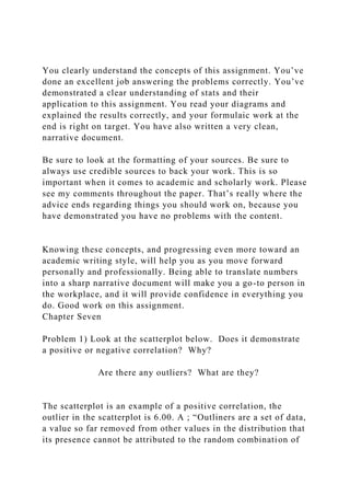
  • 7. 21.0 2.94 27.0 3.38 25.0 3.21 30.0 3.65 What is the R? What type of relationship does it indicate (strong/weak; positive/negative)? 22 3.00 32 3.78 33 3.68 21 2.94 27 3.38 25 3.21 30 3.65
  • 8. r = 0.984275 0.00 0.50 1.00 1.50 2.00 2.50 3.00 3.50 4.00 05101520253035 The relationship between the ACT and the GPA is strong, with the r being r=0.98. The point also goes from the lower left to the upper right. Go to the coefficients readout. The constant is the intercept. Under that is the ACT and that is the slope. Using the straight line formula of Y = mx + b, which you will find on page 313, you will now predict some future GPA scores: In the formula (m) is the slope; (x) is the variable that you are looking to use as a predictor; and (b) is the intercept. Predict GPA from the following ACT scores using the regression equation/straight line formula (show all your work): Using the formula x=mx + b, the slope (m-value) is 0.070391949152542 and the intercept (b-value) 1.4665042372881; x is the variable and will be used as the
  • 9. predictor. In order to get the GPA both the m-value and b value will be rounded off making the GPA: 20 Y = mx+b Y = 0.0704(20) + 1.4665 Y = 1.408 + 1.4665 Y = 2.8745 Y=2.78 25 Y = mx+b Y = 0.0704(25) + 1.4665 Y = 1.76 + 1.4665 Y = 3.2265 Y = 3.23 34 Y = mx+b Y = 0.0704(34) + 1.4665 Y = 2.3936 + 1.4665 Y = 3.8601
  • 10. Y = 3.86 Chapter Eight Show all your work Problem 1) A sample of nine students is selected from among the students taking a particular exam. The nine students were asked how much time they had spent studying for the exam and the responses (in hours) were as follows: �Correct. Be sure to cite your sources in proper APA. Why do you suppose it’s so important to back your work with credible sources? �Very good. �Be sure to cite academic sources in each section. �Again, find academic sources. Peer reviewed is essential. �Correct. Same comment re: credible sources. �These are correct.
  • 11. Slide 10 - * Active Learning Questions Copyright © 2009 Pearson Education, Inc. For use with classroom response systems Chapter 10 t Tests, Two-Way Tables, and ANOVA * Slide 10 - * This partial t-table can be used where necessary. * Slide 10 - * The t distribution can be used when finding a confidence interval for the population mean with a small sample whenever the sample comes from a symmetric population. a. True b. False
  • 12. * Slide 10 - * The t distribution can be used when finding a confidence interval for the population mean with a small sample whenever the sample comes from a symmetric population. a. True b. False * Slide 10 - * A simple random sample from a normal distribution is taken in order to obtain a 95% confidence interval for the population mean. If the sample size is 12, the sample mean is 32, and the sample standard deviation s is 9.5, what is the margin of error? a. 0.604 b. 1.74 c. 5.98 d. 6.04 *
  • 13. Slide 10 - * A simple random sample from a normal distribution is taken in order to obtain a 95% confidence interval for the population mean. If the sample size is 12, the sample mean is 32, and the sample standard deviation s is 9.5, what is the margin of error? a. 0.604 b. 1.74 c. 5.98 d. 6.04 * Slide 10 - * A 95% confidence interval for the mean of a normal population a. 0.8 b. 0.16 c. 1.6 d. 16
  • 14. * Slide 10 - * A 95% confidence interval for the mean of a normal population is found a. 0.8 b. 0.16 c. 1.6 d. 16 * Slide 10 - * The margin of error in estimating the population mean of a normal population is E = 9.3 when the sample size is 15. If the sample size had been 6 and the sample standard deviation did not change, how would the margin of error change? a. It would be smaller b. It would be larger c. It would stay the same d. Cannot be determined
  • 15. * Slide 10 - * The margin of error in estimating the population mean of a normal population is E = 9.3 when the sample size is 15. If the sample size had been 6 and the sample standard deviation did not change, how would the margin of error change? a. It would be smaller b. It would be larger c. It would stay the same d. Cannot be determined * Slide 10 - * A golfer wished to find a ball that would travel more than 200 yards when hit with his 4-iron with a club speed of 90 miles per hour. He had a golf equipment lab test a low compression ball by having a robot swing his club 9 times at the required speed. State the null and alternative hypotheses for this test. a. b.
  • 16. c. d. * Slide 10 - * A golfer wished to find a ball that would travel more than 200 yards when hit with his 4-iron with a club speed of 90 miles per hour. He had a golf equipment lab test a low compression ball by having a robot swing his club 9 times at the required speed. State the null and alternative hypotheses for this test. a. b. c. d. * Slide 10 - * Data from the test in the previous example resulted in a sample mean of 206.8 yards with a sample standard deviation of 4.6 yards. Assuming normality, find the value of the t statistic.
  • 17. Recall the mean being tested was 200 yards with 9 swings by the robot. a. –4.435 b. –13.304 c. 4.435 d. 13.304 * Slide 10 - * Data from the test in the previous example resulted in a sample mean of 206.8 yards with a sample standard deviation of 4.6 yards. Assuming normality, find the value of the t statistic. Recall the mean being tested was 200 yards with 9 swings by the robot. a. –4.435 b. –13.304 c. 4.435 d. 13.304 *
  • 18. Slide 10 - * Data from the test in the previous example resulted in a sample mean of 206.8 yards with a sample standard deviation of 4.6 yards. Assuming normality, find the critical value at the 0.05 significance level. Recall the mean being tested was 200 yards with 9 swings by the robot. a. 2.306 b. 2.262 c. 1.833 d. 1.860 * Slide 10 - * Data from the test in the previous example resulted in a sample mean of 206.8 yards with a sample standard deviation of 4.6 yards. Assuming normality, find the critical value at the 0.05 significance level. Recall the mean being tested was 200 yards with 9 swings by the robot. a. 2.306 b. 2.262 c. 1.833 d. 1.860
  • 19. * Slide 10 - * For the previous example, determine the results of a hypothesis test. a. Reject the null hypothesis. The data provide sufficient evidence that the average distance is greater than 200 yards. b. Accept the null hypothesis. The data provide sufficient evidence that the average distance is greater than 200 yards. c. Reject the null hypothesis. The data do not provide sufficient evidence that the average distance is greater than 200 yards. d. Accept the null hypothesis. The data do not provide sufficient evidence that the average distance is greater than 200 yards. * Slide 10 - * For the previous example, determine the results of a hypothesis test. a. Reject the null hypothesis. The data provide sufficient evidence that the average distance is greater than 200 yards. b. Accept the null hypothesis. The data provide sufficient evidence that the average distance is greater than 200 yards. c. Reject the null hypothesis. The data do not provide sufficient evidence that the average distance is greater than 200 yards.
  • 20. d. Accept the null hypothesis. The data do not provide sufficient evidence that the average distance is greater than 200 yards. * Slide 10 - * One hundred people are selected at random and tested for colorblindness to determine whether gender and colorblindness are independent. The following counts were observed. Find the expected value of a male who is not colorblind. a. 6.0 b. 54.0 c. 4.0 d. 36.0ColorblindNot ColorblindTotalMale95160Female13940Total1090100 *
  • 21. Slide 10 - * One hundred people are selected at random and tested for colorblindness to determine whether gender and colorblindness are independent. The following counts were observed. Find the expected value of a male who is not colorblind. a. 6.0 b. 54.0 c. 4.0 d. 36.0 ColorblindNot ColorblindTotalMale95160Female13940Total1090100 * Slide 10 - * For the previous example, here are the expected values. Find the a. 1.389 b. 1.0 c. 4.167 d. 4.0ColorblindNot ColorblindTotalMale6.054.060Female4.036.040Total10.090.010 0
  • 22. * Slide 10 - * For the previous example, here are the expected values. Find the a. 1.389 b. 1.0 c. 4.167 d. 4.0 ColorblindNot ColorblindTotalMale6.054.060Female4.036.040Total10.090.010 0
  • 23. * Slide 10 - * State the null and alternative hypothesis for the test associated with the data in the previous example. a. H0: Colorblindness and gender are independent Ha: Colorblindness and gender are related b. H0: Colorblindness and gender are dependent Ha: Colorblindness and gender are not related c. H0: Colorblindness and gender are related Ha: Colorblindness and gender are independent d. H0: Colorblindness and gender are nor related Ha: Colorblindness and gender are dependent * Slide 10 - * State the null and alternative hypothesis for the test associated with the data in the previous example. a. H0: Colorblindness and gender are independent
  • 24. Ha: Colorblindness and gender are related b. H0: Colorblindness and gender are dependent Ha: Colorblindness and gender are not related c. H0: Colorblindness and gender are related Ha: Colorblindness and gender are independent d. H0: Colorblindness and gender are nor related Ha: Colorblindness and gender are dependent * Slide 10 - * the previous example had been 4.216, state your conclusion about the relationship between gender and colorblindness. a. Reject H0. There is insufficient evidence to support the claim that colorblindness and gender are related. b. Accept H0. There is insufficient evidence to support the claim that colorblindness and gender are related. c. Reject H0. There is sufficient evidence to support the claim that colorblindness and gender are related.
  • 25. d. Accept H0. There is sufficient evidence to support the claim that colorblindness and gender are related. * Slide 10 - * able using a 0.05 the previous example had been 4.216, state your conclusion about the relationship between gender and colorblindness. a. Reject H0. There is insufficient evidence to support the claim that colorblindness and gender are related. b. Accept H0. There is insufficient evidence to support the claim that colorblindness and gender are related. c. Reject H0. There is sufficient evidence to support the claim that colorblindness and gender are related. d. Accept H0. There is sufficient evidence to support the claim that colorblindness and gender are related. * Slide 10 - * The data given were analyzed using one-way analysis or variance. The purpose of the analysis is to:
  • 26. a. determine whether the groups A, B, and C are independent. b. test the hypothesis that the population means of the three groups are equal. c. test the hypothesis that the population variances of the three groups are equal. d. test the hypothesis that the sample means of the three groups are equal.ABC292719262321252925282117 * Slide 10 - * The data given were analyzed using one-way analysis or variance. The purpose of the analysis is to: a. determine whether the groups A, B, and C are independent. b. test the hypothesis that the population means of the three groups are equal. c. test the hypothesis that the population variances of the three groups are equal. d. test the hypothesis that the sample means of the three groups are equal. ABC292719262321252925282117
  • 27. * Slide 10 - * Here are the results of the ANOVA for the previous example (question on next slide):SUMMARYGroupsCountSumsAverageVarianceA4108273 .33333B41002513.33333C48220.511.66667SUMMARYSource of VariationSSdfMSFP-valueF critBetween Groups88.7244.34.6940.04014.25649Within Groups8599.4Total173.711
  • 28. * Slide 10 - * If the significance level for the test is 0.05, which conclusion below is correct? a. The data do not provide sufficient evidence to conclude that the population means of groups A, B, and C are related. b. The data do not provide sufficient evidence to conclude that the population means of groups A, B, and C are different. c. The data do not provide sufficient evidence to conclude that the population variances of groups A, B, and C are different. d. The data do not provide sufficient evidence to conclude that the population means of groups A, B, and C are different. *
  • 29. Slide 10 - * If the significance level for the test is 0.05, which conclusion below is correct? a. The data do not provide sufficient evidence to conclude that the population means of groups A, B, and C are related. b. The data do not provide sufficient evidence to conclude that the population means of groups A, B, and C are different. c. The data do not provide sufficient evidence to conclude that the population variances of groups A, B, and C are different. d. The data do not provide sufficient evidence to conclude that the population means of groups A, B, and C are different. * x Slide 9 - * Active Learning Questions Copyright © 2009 Pearson Education, Inc. For use with classroom response systems Chapter 9 Hypothesis Testing
  • 30. * Slide 9 - * Note: Students should have their textbooks open to page 211 in the textbook and refer to Table 5.1 when answering these Active Learning Questions. * Slide 9 - * A researcher claims that less than 62% of voters favor gun control. State the null hypothesis and the alternative hypothesis for a test of significance. a. H0: p = 0.62 Ha: p > 0.62 b. H0: p < 0.62 Ha: p = 0.62 c. H0: p > 0.62 Ha: p = 0.62 d. H0: p = 0.62 Ha: p < 0.62 * Slide 9 - *
  • 31. A researcher claims that less than 62% of voters favor gun control. State the null hypothesis and the alternative hypothesis for a test of significance. a. H0: p = 0.62 Ha: p > 0.62 b. H0: p < 0.62 Ha: p = 0.62 c. H0: p > 0.62 Ha: p = 0.62 d. H0: p = 0.62 Ha: p < 0.62 * Slide 9 - * A study of a brand of “in the shell” peanuts gives the following table. A significant event at the 0.01 level is a fan getting a bag with how many peanuts? a. 25, 30, or 35 b. 25, 30, or 55 c. 35, 45, or 50 d. None of the choices# Peanuts in the bag25303540455055Probability0.0030.020.090.150.450.2170.07
  • 32. * Slide 9 - * A study of a brand of “in the shell” peanuts gives the following table. A significant event at the 0.01 level is a fan getting a bag with how many peanuts? a. 25, 30, or 35 b. 25, 30, or 55 c. 35, 45, or 50 d. None of the choices # Peanuts in the bag25303540455055Probability0.0030.020.090.150.450.2170.07 *
  • 33. Slide 9 - * The manufacturer of a refrigerator system for beer kegs produces refrigerators that are supposed to maintain a true mean temperatur pilsner. The owner of the brewery does not agree with the refrigerator manufacturer, and claims that the true mean temperature is incorrect. Assume that a hypothesis test of the claim has been conducted and that the conclusion of the test was to reject the null hypothesis. Identify the population to which the results of the test apply. a. All refrigerators produced by the manufacturer specifically to cool kegs of a particular German pilsner beer b. All refrigerators produced by the manufacturer c. All refrigerators produced by the manufacturer specifically to cool kegs of beer d. There is not sufficient description to identify the population * Slide 9 - * The manufacturer of a refrigerator system for beer kegs produces refrigerators that are supposed to maintain a true mean pilsner. The owner of the brewery does not agree with the refrigerator manufacturer, and claims that the true mean temperature is incorrect. Assume that a hypothesis test of the claim has been conducted and that the conclusion of the test was to reject the null hypothesis. Identify the population to which the results of the test apply.
  • 34. a. All refrigerators produced by the manufacturer specifically to cool kegs of a particular German pilsner beer b. All refrigerators produced by the manufacturer c. All refrigerators produced by the manufacturer specifically to cool kegs of beer d. There is not sufficient description to identify the population * Slide 9 - * A cereal company claims that the mean weight of the cereal in its packets is at least 14 oz. Assume that a hypothesis test of the claim has been conducted and that the conclusion of the test was to reject the null hypothesis. Identify the population to which the results of the test apply. a. The cereal packets that were tested b. The cereal packets of one kind manufactured by the cereal company c. The cereal packets claiming a weight of at least 14 oz d. All cereal packets manufactured by the cereal company * Slide 9 - * A cereal company claims that the mean weight of the cereal in its packets is at least 14 oz. Assume that a hypothesis test of the
  • 35. claim has been conducted and that the conclusion of the test was to reject the null hypothesis. Identify the population to which the results of the test apply. a. The cereal packets that were tested b. The cereal packets of one kind manufactured by the cereal company c. The cereal packets claiming a weight of at least 14 oz d. All cereal packets manufactured by the cereal company * Slide 9 - * In 1990, the average math SAT score for students at one school was 510. Five years later, a teacher wants to perform a hypothesis test to determine whether the average math SAT score of students at the school has changed from the 1990 mean of 510. Formulate the null and alternative hypotheses for the study described. a. b. c. d. *
  • 36. Slide 9 - * In 1990, the average math SAT score for students at one school was 510. Five years later, a teacher wants to perform a hypothesis test to determine whether the average math SAT score of students at the school has changed from the 1990 mean of 510. Formulate the null and alternative hypotheses for the study described. a. b. c. d. * Slide 9 - * The manufacturer of a refrigerator system for beer kegs produces refrigerators that are supposed to maintain a true mean pilsner. The owner of the brewery does not agree with the refrigerator manufacturer, and claims he can prove that the true mean temperature is incorrect. Assuming that a hypothesis test of the claim has been conducted and that the conclusion is to reject the null hypothesis, state the conclusion in non-technical terms. a. There is not sufficient evidence to support the claim that the mean temperature is equal to 46ºF b. There is sufficient evidence to support the claim that the
  • 37. mean temperature is equal to 46ºF c. There is not sufficient evidence to support the claim that the mean temperature is different from 46ºF d. There is sufficient evidence to support the claim that the mean temperature is different from 46ºF * Slide 9 - * The manufacturer of a refrigerator system for beer kegs produces refrigerators that are supposed to maintain a true mean pilsner. The owner of the brewery does not agree with the refrigerator manufacturer, and claims he can prove that the true mean temperature is incorrect. Assuming that a hypothesis test of the claim has been conducted and that the conclusion is to reject the null hypothesis, state the conclusion in non-technical terms. a. There is not sufficient evidence to support the claim that the mean temperature is equal to 46ºF b. There is sufficient evidence to support the claim that the mean temperature is equal to 46ºF c. There is not sufficient evidence to support the claim that the mean temperature is different from 46ºF d. There is sufficient evidence to support the claim that the mean temperature is different from 46ºF *
  • 38. Slide 9 - * - value, determine whether the alternate hypothesis is supported and give a reason for your conclusion. a. Ha is not supported; is less than 1 standard deviation above the claimed area b. Ha is not supported; is more than 4 standard deviations above the claimed area c. Ha is supported; is less than 1 standard deviation above the claimed area d. Ha is supported; is more than 4 standard deviations above the claimed area * Slide 9 - * - value, determine whether the alternate hypothesis is supported and give a reason for your conclusion. a. Ha is not supported; is less than 1 standard deviation above the claimed area
  • 39. b. Ha is not supported; is more than 4 standard deviations above the claimed area c. Ha is supported; is less than 1 standard deviation above the claimed area d. Ha is supported; is more than 4 standard deviations above the claimed area * Slide 9 - * z = – -value for the test? a. 6.68 b. 93.32 c. 0.0668 d. None of the above *
  • 40. Slide 9 - * z = – aimed value; What is the P-value for the test? a. 6.68 b. 93.32 c. 0.0668 d. None of the above * Slide 9 - * A health insurer has determined that the “reasonable and customary” fee for a certain medical procedure is $1200. They suspect that the average fee charged by one particular clinic for this procedure is higher than $1200. The insurer wants to perform a hypothesis test to determine whether their suspicion is correct. The mean fee charged by the clinic for a random sample of 65 patients receiving this procedure was $1280. Do the data provide sufficient evidence to conclude that the mean fee charged by this particular clinic is higher than $1200? Use a significance level of 0.01. Assume that σ = $220. a. The z-score of 2.93 provides sufficient evidence to conclude that the mean fee charged for the procedure is greater than $1200 b. The z-score of 0.363 does not provide sufficient evidence to conclude that the mean fee charged for the procedure is
  • 41. greater than $1200 c. The P-value of 0.363 does not provide sufficient evidence to conclude that the mean fee charged for the procedure is greater than $1200 d. The P-value of 0.045 provides sufficient evidence to conclude that the mean fee charged for the procedure is greater than $1200 * Slide 9 - * A health insurer has determined that the “reasonable and customary” fee for a certain medical procedure is $1200. They suspect that the average fee charged by one particular clinic for this procedure is higher than $1200. The insurer wants to perform a hypothesis test to determine whether their suspicion is correct. The mean fee charged by the clinic for a random sample of 65 patients receiving this procedure was $1280. Do the data provide sufficient evidence to conclude that the mean fee charged by this particular clinic is higher than $1200? Use a significance level of 0.01. Assume that σ = $220. a. The z-score of 2.93 provides sufficient evidence to conclude that the mean fee charged for the procedure is greater than $1200 b. The z-score of 0.363 does not provide sufficient evidence to conclude that the mean fee charged for the procedure is greater than $1200 c. The P-value of 0.363 does not provide sufficient evidence to conclude that the mean fee charged for the procedure is greater than $1200 d. The P-value of 0.045 provides sufficient evidence to conclude that the mean fee charged for the procedure is greater
  • 42. than $1200 * Slide 9 - * A long-distance telephone company claims that the mean duration of long-distance telephone calls originating in one town was not equal to 9.4 minutes, which is the average for the state. Determine the null and alternative hypotheses for the test described. a. b. c. d. * Slide 9 - * A long-distance telephone company claims that the mean duration of long-distance telephone calls originating in one town was not equal to 9.4 minutes, which is the average for the state. Determine the null and alternative hypotheses for the test described. a.
  • 43. b. c. d. * Slide 9 - * A manufacturer wishes to test the claim that one of its pancake mixes has a mean weight that does not equal 24 ounces as advertised. Determine the conclusion of the hypothesis test assuming that the results of the sampling lead to rejection of the null hypothesis. a. Support the claim that the mean is greater than 24 oz b. Support the claim that the mean is not equal to 24 oz c. Support the claim that the mean is equal to 24 oz d. Support the claim that the mean is less than 24 oz * Slide 9 - * A manufacturer wishes to test the claim that one of its pancake
  • 44. mixes has a mean weight that does not equal 24 ounces as advertised. Determine the conclusion of the hypothesis test assuming that the results of the sampling lead to rejection of the null hypothesis. a. Support the claim that the mean is greater than 24 oz b. Support the claim that the mean is not equal to 24 oz c. Support the claim that the mean is equal to 24 oz d. Support the claim that the mean is less than 24 oz * Slide 9 - * The standard score for a two-tailed test is 2.0. What is the P- value? a. 0.9772 b. 0.0456 c. 0.0228 d. 97.72 * Slide 9 - *
  • 45. The standard score for a two-tailed test is 2.0. What is the P- value? a. 0.9772 b. 0.0456 c. 0.0228 d. 97.72 * Slide 9 - * A two-tailed test is conducted at the 5% significance level. What is the smallest z-score listed below that results in rejection of the null hypothesis? a. 1.17 b. 1.58 c. 1.81 d. 2.89 * Slide 9 - *
  • 46. A two-tailed test is conducted at the 5% significance level. What is the smallest z-score listed below that results in rejection of the null hypothesis? a. 1.17 b. 1.58 c. 1.81 d. 2.89 * Slide 9 - * A two-tailed test is conducted at the 10% significance level. What is the z-score closest to zero in the list that will result in rejection of the null hypothesis? a. 1.19 b. –1.54 c. –1.84 d. 2.59 *
  • 47. Slide 9 - * A two-tailed test is conducted at the 10% significance level. What is the z-score closest to zero in the list that will result in rejection of the null hypothesis? a. 1.19 b. –1.54 c. –1.84 d. 2.59 * Slide 9 - * In 1990, the average duration of long-distance telephone calls originating in one town was 9.4 minutes. A telephone company wants to perform a hypothesis test to determine whether the average duration of long-distance phone calls has changed. The mean duration for a random sample of 50 calls originating in the town was 8.6 minutes. Does the data provide sufficient evidence significance level 0.01, & σ = 4.2 minutes. a. P-value greater than 0.01; sufficient evidence to accept the null hypothesis and conclude that the mean call duration has changed b. P-value less than 0.01; sufficient evidence to reject the null hypothesis and conclude that the mean call duration has changed c. P-value greater than 0.01; insufficient evidence to reject
  • 48. the null hypothesis and conclude that the mean call duration has changed d. P-value greater than 0.01; sufficient evidence to reject the null hypothesis and conclude that the mean call duration has changed * Slide 9 - * In 1990, the average duration of long-distance telephone calls originating in one town was 9.4 minutes. A telephone company wants to perform a hypothesis test to determine whether the average duration of long-distance phone calls has changed. The mean duration for a random sample of 50 calls originating in the town was 8.6 minutes. Does the data provide sufficient evidence significance level 0.01, & σ = 4.2 minutes. a. P-value greater than 0.01; sufficient evidence to accept the null hypothesis and conclude that the mean call duration has changed b. P-value less than 0.01; sufficient evidence to reject the null hypothesis and conclude that the mean call duration has changed c. P-value greater than 0.01; insufficient evidence to reject the null hypothesis and conclude that the mean call duration has changed d. P-value greater than 0.01; sufficient evidence to reject the null hypothesis and conclude that the mean call duration has changed
  • 49. * Slide 9 - * At one school, the average amount of time that tenth-graders spend watching television each week is 21 hours. The principal introduces a campaign to encourage the students to watch less television. One year later, the principal wants to perform a hypothesis test to determine whether the average amount of time spent watching television per week has decreased. The that the results of the sampling lead to non-rejection of the null hypothesis. Classify that conclusion as a Type I error, a Type II error, or a correct decision, if in fact the mean amount of time, a. Type I error b. Correct decision c. Type II error * Slide 9 - * At one school, the average amount of time that tenth-graders spend watching television each week is 21 hours. The principal introduces a campaign to encourage the students to watch less television. One year later, the principal wants to perform a hypothesis test to determine whether the average amount of time spent watching television per week has decreased. The that the results of the sampling lead to non-rejection of the null hypothesis. Classify that conclusion as a Type I error, a Type II error, or a correct decision, if in fact the mean amount of time,
  • 50. a. Type I error b. Correct decision c. Type II error * Slide 9 - * A health insurer has determined that the “reasonable and customary” fee for a certain medical procedure is $1200. They suspect that the average fee charged by one particular clinic for this procedure is higher than $1200. The insurer wants to perform a hypothesis test to determine whether their suspicion Explain the meaning of a correct decision. a. b. c. d. * Slide 9 - * A health insurer has determined that the “reasonable and customary” fee for a certain medical procedure is $1200. They suspect that the average fee charged by one particular clinic for
  • 51. this procedure is higher than $1200. The insurer wants to perform a hypothesis test to determine whether their suspicion Explain the meaning of a correct decision. a. b. c. d. * Slide 9 - * The average diastolic blood pressure of a group of men suffering from high blood pressure is 96 mmHg. During a clinical trial, the men receive a medication, which it is hoped, will lower their blood pressure. After three months, the researcher wants to perform a hypothesis test to determine whether the average diastolic blood pressure of the men has a. b. Fa c. d.
  • 52. * Slide 9 - * The average diastolic blood pressure of a group of men suffering from high blood pressure is 96 mmHg. During a clinical trial, the men receive a medication, which it is hoped, will lower their blood pressure. After three months, the researcher wants to perform a hypothesis test to determine whether the average diastolic blood pressure of the men has a. b. Failing to c. d. * Slide 9 - * A random sample of 139 forty-year-old men contains 26% smokers. Use Table 5.1 to estimate the P-value for a test of the claim that the percentage of forty-year-old men that smoke is 22%. a. 0.2542 b. 0.1401
  • 53. c. 0.2802 d. 0.1271 * Slide 9 - * A random sample of 139 forty-year-old men contains 26% smokers. Use Table 5.1 to estimate the P-value for a test of the claim that the percentage of forty-year-old men that smoke is 22%. a. 0.2542 b. 0.1401 c. 0.2802 d. 0.1271 * Slide 9 - * According to a recent poll 53% of Americans would vote for the incumbent president. If a random sample of 100 people results in 45% who would vote for the incumbent, test the hypothesis that the actual percentage is 53%. Use a 0.10 significance level
  • 54. and a two-tailed test. a. Do not reject the null hypothesis; insufficient evidence to reject the claim that 53% of Americans would vote for the incumbent president. b. Do not reject the null hypothesis; sufficient evidence to reject the claim that 53% of Americans would vote for the incumbent president. c. Reject the null hypothesis; insufficient evidence to reject the claim that 53% of Americans would vote for the incumbent president. d. Reject the null hypothesis; sufficient evidence to reject the claim that 53% of Americans would vote for the incumbent president. * Slide 9 - * According to a recent poll 53% of Americans would vote for the incumbent president. If a random sample of 100 people results in 45% who would vote for the incumbent, test the hypothesis that the actual percentage is 53%. Use a 0.10 significance level and a two-tailed test. a. Do not reject the null hypothesis; insufficient evidence to reject the claim that 53% of Americans would vote for the incumbent president. b. Do not reject the null hypothesis; sufficient evidence to reject the claim that 53% of Americans would vote for the incumbent president. c. Reject the null hypothesis; insufficient evidence to reject the claim that 53% of Americans would vote for the incumbent president. d. Reject the null hypothesis; sufficient evidence to reject the
  • 55. claim that 53% of Americans would vote for the incumbent president. * x = 2 3 . 8 , x Data File 5 Chapter Nine Show all work Problem 1) A skeptical paranormal researcher claims that the proportion of Americans that have seen a UFO is less than 1 in every one thousand. State the null hypothesis and the alternative hypothesis for a test of significance. Problem 2) At one school, the average amount of time that tenth-graders spend watching television each week is 18.4 hours. The principal introduces a campaign to encourage the students to watch less television. One year later, the principal wants to perform a hypothesis test to determine whether the average amount of time spent watching television per week has decreased. Formulate the null and alternative hypotheses for the study described.
  • 56. Problem 3) A two-tailed test is conducted at the 5% significance level. What is the P-value required to reject the null hypothesis? Problem 4) A two-tailed test is conducted at the 5% significance level. What is the right tail percentile required to reject the null hypothesis? Problem 5) What is the difference between an Type I and a Type II error? Provide an example of both. Chapter 10 Show all work Problem 1) Steven collected data from 20 college students on their emotional responses to classical music. Students listened to two 30-second segments from “The Collection from the Best of Classical Music.” After listening to a segment, the students rated it on a scale from 1 to 10, with 1 indicating that it “made them very sad” to 10 indicating that it “made them very happy.” Steve computes the total scores from each student and created a variable called “hapsad.” Steve then conducts a one-sample t- test on the data, knowing that there is an established mean for the publication of others that have taken this test of 6. The following is the scores: 5.0 5.0 10.0 3.0
  • 57. 13.0 13.0 7.0 5.0 5.0 15.0 14.0 18.0 8.0 12.0 10.0 7.0 3.0 15.0 4.0 3.0 a) Conduct a one-sample t-test. What is the t-test score? What is the mean? Was the test significant? If it was significant at what P-value level was it significant?
  • 58. b) What is your null and alternative hypothesis? Given the results did you reject or fail to reject the null and why? (Use instructions on page 437 of your textbook, under Hypothesis Tests with the t Distribution to conduct SPSS or Excel analysis). Problem 2) Billie wishes to test the hypothesis that overweight individuals tend to eat faster than normal-weight individuals. To test this hypothesis, she has two assistants sit in a McDonald’s restaurant and identify individuals who order the Big Mac special for lunch. The Big Mackers as they become known are then classified by the assistants as overweight, normal weight, or neither overweight nor normal weight. The assistants identify 10 overweight and 10 normal weight Big Mackers. The assistants record the amount of time it takes them to eight the Big Mac special. 1.0 585.0 1.0 540.0 1.0 660.0 1.0 571.0
  • 60. 2.0 675.0 2.0 635.0 2.0 672.0 2.0 606.0 2.0 789.0 2.0 806.0 2.0 600.0 a) Compute an independent-samples t-test on these data. Report the t-value and the p values. Where the results significant? (Do the same thing you did for the t-test above, only this type when you go to compare means, click on independent samples t-test. When you enter group variable into grouping variable area, it will ask you to define the variables. Click define groups and place the number 1 into 1 and the number 2 into 2). b) What is the difference between the mean of the two groups? What is the difference is standard deviation?
  • 61. c) What is the null and alternative hypothesis? Do the data results lead you to reject or fail to reject the null hypothesis? d) What do the results tell you? Problem 3) Lilly collects data on a sample of 40 high school students to evaluate whether the proportion of female high school students who take advanced math courses in high school varies depending upon whether they have been raised primarily by their father or by both their mother and their father. Two variables are found below in the data file: math (0 = no advanced math and 1 = some advanced math) and Parent (1= primarily father and 2 = father and mother). Parent Math 1.0 0.0 1.0 0.0 1.0 0.0 1.0 0.0
  • 66. a) Conduct a crosstabs analysis to examine the proportion of female high school students who take advanced math courses is different for different levels of the parent variable. b) What percent female students took advanced math class c) What percent of female students did not take advanced math class when females were raised by just their father? d) What are the Chi-square results? What are the expected and the observed results that were found? Are they results of the Chi-Square significant? What do the results mean? e) What were your null and alternative hypotheses? Did the results lead you to reject or fail to reject the null and why? Problem 4) This problem will introduce the learner into a technique called Analysis of Variance. For this course we will only conduct a simple One-Way ANOVA and touch briefly on the important elements of this technique. The One-Way ANOVA is an extension of the independent –t test that can only look at two independent sample means. We can use the One-Way ANOVA to look at three or more independent sample means. Use the following data to conduct a One-Way ANOVA: Scores Group 1 1 2 1
  • 67. 3 1 2 2 3 2 4 2 4 3 5 3 6 3 Notice the group (grouping) variable, which is the independent variable or factor is made up of three different groups. The scores are the dependent variable. Use the instructions for conduction an ANOVA on page 438 of the text for SPSS or Excel.
  • 68. a) What is the F-score; Are the results significant, and if so, at what level (P-value)? b) If the results are significant to the following: Click analyze, then click Compare Means, and then select one-way ANOVA like you did previously. Now click Post Hoc. In this area check Tukey. If there is a significant result, we really do not know where it is. Is it between group 1 and 2, 1 and 3, or 2 and 3? Post hoc tests let us isolate where the level of significance was. So if the results come back significant, conduct the post hoc test as I mentioned above and explain where the results were significant. c) What do the results obtained from the test mean? Activity 7 Section 4: Hypothesis Testing, T-Tests, Cross-Tabulations, and Chi-Square Suppose someone makes the claim that it rains between June and August more than any other months in the year. How does one know the statement is true? In statistics, we answer such questions through hypothesis testing. Researchers collect rain fall data over a period of years and run various statistical tests. Some of the methods to prove the statement are completed by employing various statistical tools such as t-test, cross- tabulations, Chi-Square, ANOVA and the like. In this section, you will learn the difference between a null and an alternative hypothesis and how to state a hypothesis. You will explore the differences between one- and two-tailed testing, determine the importance of the p-value, and understand Type I and Type II errors in the context of hypothesis.
  • 69. Required Reading: Please refer to the Activity Resources section within each activity for required readings. Assignment 7 Hypothesis Testing One of the most important uses of statistics is the analyzing of data from studies. Business researchers want to do more that describe samples statistically. They want to know if variances are likely due to chance or to real differences between groups. Similarly, governmental agencies use data to determine issues such as the labor situation, and to track effects of policies on citizens. In this activity, you will work with basic statistics used to compare groups. This will help you gain proficiency in understanding, developing and testing hypotheses. Activity Resources · Bennett, J. O., Briggs, W. L., & Triola, M. F. (2014)., Chapters 9 and 10 Please view these four short videos on important concepts that are explored in this activity (Two are hyperlinks and two are embedded). · Chi Square - Dr. A.G. Picciano (click on link) · Estimation of a Population Proportion, Part 2 of 2 (click on link) · Hypothesis Testing, Part 1 of 2 (embedded below) · T-test - Dr. A.G. Picciano (embedded below)
  • 70. ________________________________________ Chapter Practice Questions After you complete the textbook readings, check your understanding of the main concepts by reviewing the chapter review questions in the attached PowerPoint files. Be sure to revisit appropriate sections of the textbook if you find that you need more review. While these questions are not a graded part of this activity, they are important because they will help you monitor your learning as you progress through the course. · Chapter 9 PowerPoint.ppt · Chapter 10 PowerPoint.ppt ________________________________________ Main Task: Complete Application Questions and Problems Download Data File 5 and complete the problems and questions as presented. Show your work (either your hand calculations or your statistical program output). You may either scan your handwritten work and submit it as a low-resolution graphic, type your answers directly into the document, or cut and paste your work into a Word file. Be sure to name the file using the proper NCU naming conventions before its submittal. Support your paper with a minimum of three (3) scholarly resources. In addition to these specified resources, other appropriate scholarly resources, including older articles, may be included. Length: 5-7 pages not including title and reference pages, may include spreadsheets Your response should demonstrate thoughtful consideration of the ideas and concepts that are presented in the course and provide new thoughts and insights relating directly to this topic. Your response should reflect scholarly writing and current APA standards where appropriate. Be sure to adhere to Northcentral
  • 71. University's Academic Integrity Policy. Submit your document in the Course Work area below the Activity screen. Learning Outcomes: 8, 9, 10 Assignment Outcomes Calculate and utilize confidence intervals and margin of error in population estimation results. Determine alpha (p-values) values and interpret p-levels as related to statistical significance. Utilize statistical software such as Excel to conduct data analysis. Course Work Upload New Coursework